PARTITION CLUSTERING OF
HIGH DIMENSIONAL LOW SAMPLE SIZE DATA
BASED ON P-VALUES
by
GEORGE FREITAS VON BORRIES
B.A., Universidade de Bras´ılia, Brazil, 1990
M.S., Texas A&M University, USA, 2003
AN ABSTRACT OF A DISSERTATION
submitted in partial fulfillment of the
requirements for the degree
DOCTOR OF PHILOSOPHY
Department of Statistics
College of Arts and Sciences
KANSAS STATE UNIVERSITY
Manhattan, Kansas
2008
Abstract
This thesis introduces a new partitioning algorithm to cluster variables in high dimen-sional low sample size (HDLSS) data and high dimendimen-sional longitudinal low sample size (HDLLSS) data. HDLSS data contain a large number of variables with small number of replications per variable, and HDLLSS data refer to HDLSS data observed over time.
Clustering technique plays an important role in analyzing high dimensional low sample size data as is seen commonly in microarray experiment, mass spectrometry data, pattern recognition. Most current clustering algorithms for HDLSS and HDLLSS data are adapta-tions from traditional multivariate analysis, where the number of variables is not high and sample sizes are relatively large. Current algorithms show poor performance when applied to high dimensional data, especially in small sample size cases. In addition, available algo-rithms often exhibit poor clustering accuracy and stability for non-normal data. Simulations show that traditional clustering algorithms used in high dimensional data are not robust to monotone transformations.
The proposed clustering algorithm PPCLUST is a powerful tool for clustering HDLSS data, which uses p-values from nonparametric rank tests of homogeneous distribution as a measure of similarity between groups of variables. Inherited from the robustness of rank procedure, the new algorithm is robust to outliers and invariant to monotone transformations of data. PPCLUSTEL is an extension of PPCLUST for clustering of HDLLSS data. A nonparametric test of no simple effect of group is developed and the p-value from the test is used as a measure of similarity between groups of variables.
PPCLUST and PPCLUSTEL are able to cluster a large number of variables in the presence of very few replications and in case of PPCLUSTEL, the algorithm require neither a large number nor equally spaced time points. PPCLUST and PPCLUSTEL do not suffer from loss of power due to distributional assumptions, general multiple comparison problems and difficulty in controlling heterocedastic variances. Applications with available data from previous microarray studies show promising results and simulations studies reveal that the algorithm outperforms a series of benchmark algorithms applied to HDLSS data exhibiting high clustering accuracy and stability.
PARTITION CLUSTERING OF
HIGH DIMENSIONAL LOW SAMPLE SIZE DATA
BASED ON P-VALUES
by
GEORGE FREITAS VON BORRIES
B.A., Universidade de Bras´ılia, Brazil, 1990
M.S., Texas A&M University, USA, 2003
A DISSERTATION
submitted in partial fulfillment of the
requirements for the degree
DOCTOR OF PHILOSOPHY
Department of Statistics
College of Arts and Sciences
KANSAS STATE UNIVERSITY
Manhattan, Kansas
2008
Approved by: Major Professor Haiyan Wang
Copyright
George Freitas von Borries
Abstract
This thesis introduces a new partitioning algorithm to cluster variables in high dimen-sional low sample size (HDLSS) data and high dimendimen-sional longitudinal low sample size (HDLLSS) data. HDLSS data contain a large number of variables with small number of replications per variable, and HDLLSS data refer to HDLSS data observed over time.
Clustering technique plays an important role in analyzing high dimensional low sample size data as is seen commonly in microarray experiment, mass spectrometry data, pattern recognition. Most current clustering algorithms for HDLSS and HDLLSS data are adapta-tions from traditional multivariate analysis, where the number of variables is not high and sample sizes are relatively large. Current algorithms show poor performance when applied to high dimensional data, especially in small sample size cases. In addition, available algo-rithms often exhibit poor clustering accuracy and stability for non-normal data. Simulations show that traditional clustering algorithms used in high dimensional data are not robust to monotone transformations.
The proposed clustering algorithm PPCLUST is a powerful tool for clustering HDLSS data, which uses p-values from nonparametric rank tests of homogeneous distribution as a measure of similarity between groups of variables. Inherited from the robustness of rank procedure, the new algorithm is robust to outliers and invariant to monotone transformations of data. PPCLUSTEL is an extension of PPCLUST for clustering of HDLLSS data. A nonparametric test of no simple effect of group is developed and the p-value from the test is used as a measure of similarity between groups of variables.
PPCLUST and PPCLUSTEL are able to cluster a large number of variables in the presence of very few replications and in case of PPCLUSTEL, the algorithm require neither a large number nor equally spaced time points. PPCLUST and PPCLUSTEL do not suffer from loss of power due to distributional assumptions, general multiple comparison problems and difficulty in controlling heterocedastic variances. Applications with available data from previous microarray studies show promising results and simulations studies reveal that the algorithm outperforms a series of benchmark algorithms applied to HDLSS data exhibiting high clustering accuracy and stability.
Table of Contents
Table of Contents vi
List of Figures viii
List of Tables xi Acknowledgements xii Dedication xiii 1 Introduction 1 1.1 Background . . . 3 1.2 Contribution . . . 8 2 Literature Review 10 2.1 Review of Proximity Measures . . . 10
2.2 Review of Clustering Algorithms . . . 12
2.2.1 Partitional Clustering Methods . . . 12
2.2.2 Hierarchical Clustering Methods . . . 15
2.2.3 Fuzzy clustering . . . 19
2.2.4 Model-Based Clustering (MCLUST) . . . 20
2.2.5 ANOVA methods in clustering analysis . . . 24
2.3 Cluster Quality by Adjusted Rand Index . . . 26
3 Partition Clustering of HDLSS Data Based on p-Values 28 3.1 The Nonparametric Test of No Group Effect . . . 30
3.1.1 Type I Error Rate . . . 31
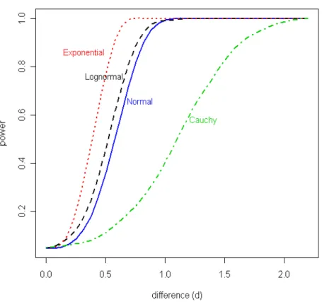
3.1.2 Power Curves . . . 33
3.2 Partition Clustering Algorithm Based on p-Values . . . 33
4 Simulations and Properties of PPCLUST in Replicated Data 38 4.1 Clustering Simulations with HDLSS Data . . . 38
4.1.1 Study I: Symmetric Groups . . . 40
4.1.2 Study II: Asymmetric Groups . . . 42
4.1.3 Results . . . 43
5 Applications of PPCLUST in Microarray Data 52
5.1 Real Data Study I: Clustering Genes in Colorectal Cancer . . . 53
5.2 Real Data Study II: Cellular Gene Expression upon HIV data . . . 63
6 Partition Clustering of HDLLSS Data Based on p-Values 66 6.1 Introduction . . . 66
6.2 Theory Development for Testing No Simple Effect of Group in HDLLSS Data 67 6.3 Simulation Study on Performance of The Test . . . 79
6.3.1 Type I Error Rate . . . 79
6.3.2 Power Curves . . . 80
6.4 Partition Clustering of HDLLSS Data Based on p-Values . . . 82
6.4.1 Performance on Simulated Data and Comparison with MCLUST . . . 82
6.4.2 Comparison to Other Methods . . . 86
7 Conclusions 88 7.1 Future Research . . . 91
Bibliography 94 A Basics of Microarray Technology 107 B SAS Macros 120 B.1 Macro PPCLUST for HDLSS data . . . 120
B.1.1 SAS Code . . . 121
B.2 Macro PPCLUSTEL for HDLLSS data . . . 128
B.2.1 SAS Code . . . 129
B.3 Macro ADJRAND for Adjusted Rand Index . . . 137
List of Figures
1.1 Diagram of clustering algorithms (Gan et al. [34]). . . 6 2.1 Example of two dimensional SOM grid for a microarray data produced with
R package. . . 15 2.2 Agglomerative (left) and divisive hierarchical (right) dendograms for the same
dataset. Agglomerative dendogram should be read from bottom to top graph and divisive should read in opposite direction. . . 16 2.3 Dataset with two intermediate objects (6 and 13). Example generate in R
language, based on KaufmanRousseeuw [52]. . . 20 2.4 BIC comparison of different models with different number of components in
clustering of a data. The covariance structures considered are EII (spherical with equal variance), VII (spherical unconstrained), EEI (diagonal with equal variance), VEI (diagonal with equal shape), EVI (diagonal with equal volume) , VVI (diagonal unconstrained), EEE (ellipsoidal with equal variance), EEV (ellipsoidal with equal volume and shape), VEV (ellipsoidal with equal shape) and VVV (ellipsoidal unconstrained). The best model is VEV with 2 clusters. 22 2.5 Example of coordinate projections of clustered objects showing clustering
(named as classification) and uncertainty of allocation. . . 23 3.1 Achieved power for HDLSS data withα= 0.05, considering shifted differences
in mean (d) in a group of 100 factor levels in a total of 2000 factor levels and data generated from four distributions: Normal(0,1) (continuous line in blue), Lognormal(0,1) (dashed line in black), Exponential(1) (dotted line in red) and Cauchy(0,1) (dotted-dashed line in green). . . 34 3.2 PPCLUST block diagram. In the diagram nf stands for “number of
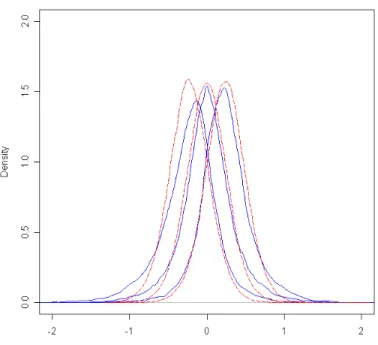
fac-tors” and g for “group label”. Group 0 is reserved to factors that cannot be allocated to any created group. . . 37 4.1 Original (continuous blue line) and simulated (dashed red line) density
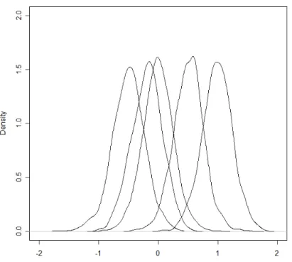
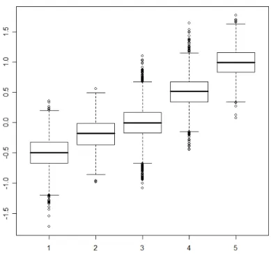
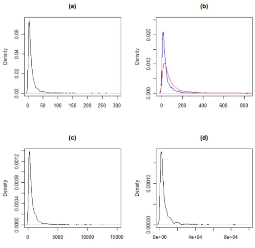
func-tions for three groups of genes in colorectal expression data . . . 40 4.2 Study I: Density functions used to generate groups of data. . . 41 4.3 Study I: Boxplots of generated data for each group. . . 42 4.4 Study II: Density plots for simulated groups, where (a) shows group 1, (b)
shows groups 2 (blue tall curve) and 3 (red short curve), (c) group 4, and (d) group 5. Groups separated into 4 plots due to large difference in their respective ranges. . . 43
4.5 Boxplots of Adjusted Rand Index for PPCLUST and 10 other algorithms, over 200 simulated datasets and considering different sample sizes. Generated
groups from symmetric distributions (Study I). . . 45
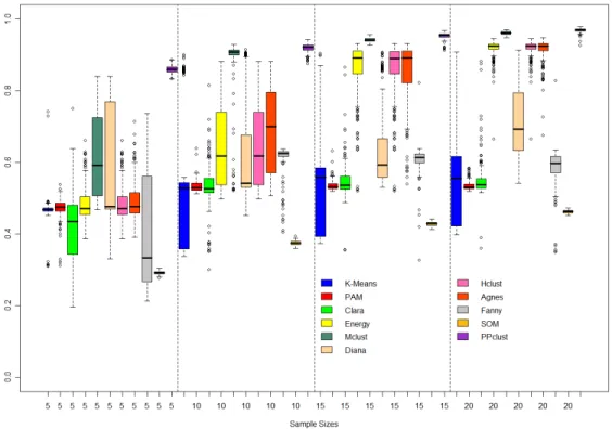
4.6 Boxplots of Adjusted Rand Index for PPCLUST and 10 other algorithms, over 200 simulated datasets and considering different sample sizes. Generated groups from asymmetric distributions (Study II). . . 47
5.1 Areas of development of colorectal cancer (nlm.nih.gov/medilineplus) . . . . 54
5.2 Polyp in colon wall (endoatlas.com) . . . 54
5.3 Heatmap for Adenoma-Normal Tissues. . . 57
5.4 Heatmap for Grouped Adenoma-Normal Tissues. . . 58
5.5 PCA Plot of Adenoma-Normal Tissue Clusters. . . 59
5.6 Heatmap for Adenocarcinoma-Normal Tissues. . . 60
5.7 Heatmap for Grouped Adenocarcinoma-Normal Tissues. . . 61
5.8 PCA Plot of Adenocarcinoma-Normal Tissue Clusters. . . 62
5.9 Stylized rendering of a cross section of the human immunodeficiency virus (Wikipedia). . . 64
5.10 Heatmap for original HIV data. . . 65
5.11 Heatmap for grouped HIV data. Genes ordered by groups. . . 65
6.1 Achieved power for HDLLSS data with α = 0.05, considering shifted differ-ences in two groups according to three cases: P200 (continuous line in blue) has 200 shifted factor levels; P100 (dashed line in red) has 100 shifted factor levels; and P050 (dotted line in black) has 50 shifted factor levels. . . 81
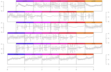
6.2 Profile plot for simulated longitudinal data. Gene expression levels in vertical axis and time points in horizontal axis. (a) All replicated factor levels. (b) Factor levels in group 1. (c) Factor levels in group 2. (d) Factor levels in group 3. (e) Factor levels in group 4. (f) Factor levels in group 5. . . 83
6.3 Boxplots for ARI in 2000 simulations using PPCLUSTEL and MCLUST to cluster generated data. . . 84
A.1 DNA double helix molecule base pairing schematic (Access Excellence at the National Health Museum, www.accessexcellence.org). . . 108
A.2 The Central Dogma of Molecular Biology (Access Excellence at the National Health Museum, www.accessexcellence.org). . . 109
A.3 Nothern blot slide superposed to microarray slide. Copyright cUniversity of North Carolina at Chapell Hill and A. Malcom Campbell. . . 109
A.4 Groups of cells exposed to different conditions. Copyright cUniversity of North Carolina at Chapell Hill and A. Malcom Campbell. . . 110
A.5 Growth of cells under two experimental conditions. Copyright cUniversity of North Carolina at Chapell Hill and A. Malcom Campbell. . . 111
A.6 Isolation of mRNA. Copyright cUniversity of North Carolina at Chapell Hill and A. Malcom Campbell. . . 112
A.7 Green and red dyes in transcription process. Copyright cUniversity of North Carolina at Chapell Hill and A. Malcom Campbell. . . 113 A.8 Labeled cDNA. Copyright cUniversity of North Carolina at Chapell Hill and
A. Malcom Campbell. . . 114 A.9 Combined cDNAs in preparation for hybridization process. Copyright cUniversity
of North Carolina at Chapell Hill and A. Malcom Campbell. . . 115 A.10 Washing off unbound cDNAs. Copyright cUniversity of North Carolina at
Chapell Hill and A. Malcom Campbell. . . 116 A.11 Merging of image from 3 scanned genes. Copyright cUniversity of North
Carolina at Chapell Hill and A. Malcom Campbell. . . 117 A.12 Different levels of gene expression in a microarray. Copyright cUniversity of
North Carolina at Chapell Hill and A. Malcom Campbell. . . 118 A.13 Microarray with expression of thousands of genes. Copyright cUniversity of
List of Tables
1.1 High dimensional replicated data layout. Herea → ∞and ni ≥2. . . 7
1.2 High dimensional replicated data layout in longitudinal design. Herea→ ∞ and ni ≥2, tj ≥2. . . 7
2.1 Contingency Table of clustering agreement. . . 26
2.2 Contingency Table of clustering agreement of 2000 clustered objects. . . 27
3.1 High dimensional data layout, where a→ ∞ and ni ≥2. . . 30
3.2 Estimated levels for one-way ANOVA . . . 32
4.1 Mean and standard deviations (std) of Adjusted Rand Index for PPCLUST and 10 other algorithms, over 200 simulated datasets and considering different sample sizes. Generated groups from symmetric distributions (Study I). . . . 44
4.2 Mean and standard deviations (std) of Adjusted Rand Index for PPCLUST and 10 other algorithms, over 200 simulated datasets and considering different sample sizes. Generated groups from asymmetric distributions (Study II). . . 46
4.3 Compilation time, in seconds, for PPCLUST and 4 other algorithms: PAM, MCLUST, HCLUST, and Energy. Datasets with 4000 factors and equal sam-ple sizes. . . 48
4.4 Number of groups and group sizes for different thresholds (α levels) in a real data example. . . 49
5.1 Distribution of 1038 genes present in both Adenoma and Adenocarcinoma tissue types. Genes in group 0 are genes not grouped by PPCLUST, and genes in group 4 are not expressed in either tissue types. . . 63
6.1 Data structure in longitudinal repeated measures design. . . 68
6.2 Estimated levels for test of no single effect. . . 80
6.3 Execution time of PPCLUSTEL and MCLUST for data with different number of factor levels. MCLUST is considered in two situations: (a) number of groups specified, (b) number of groups not specified. . . 85
B.1 High dimensional replicated data set layout. Here a→ ∞ and ni ≥2. . . 121
Acknowledgments
There are many people I want to acknowledge. First, my advisor Dr. Haiyan Wang. I would like to thank her for accepting the challenge of having as her first PhD student someone working in another country. Thank you for your guidance.
In addition, I would like to thank the other members of my thesis committee: Dr. John Boyer, Dr. James Higgins, Dr. Dallas Johnson, Dr. Karen Garrett and Dr. Mitchell Neilsen. My appreciation for all your suggestions and deep interest in my work. My special thanks to Dr. John Boyer, a friend of all students who works hard to help them succeed in their graduate studies. Thanks also to Pam Schierer, another person that made a difference when I was in Kansas State University.
My deepest thanks also to Dr. Donna Davis, Dr. Susana L. Valdovinos and Dr. Carol W. Shanklin for their hard work in helping me in some dificult moments.
I really consider Kansas State University and Kansas as my home in america. Among all those people who made it possible, I would mostly like to thank my close friends Robert Poulson, Mike Anderson and Samuel Wilson who, together with their families, adopted me while in KSU. They made me understand better, appreciate and enjoy the american culture. I made other great friends at KSU. I would like to give special thanks to F´atima, Paulo, Paulinha and Lucas for their friendly solicitude towards me and my family. I would also like to thank William Dall’ Acqua, Frank and Tania for their loving support.
I am also very grateful to my colleagues in Universidade of Bras´ılia. Special thanks to Maria Teresa Le˜ao Costa, Raul Yukishiro Matsushita and Geraldo da Silva e Souza.
Thanks also to Conselho Nacional de Desenvolvimento Cient´ıfico e Tecnol´ogico (CNPq)
for the partial support in the first years of my graduate studies, and Universidade de Bras´ılia for the support during my studies.
Besides, my thanks to the most important people in this journey and in all my life: my family. To my wonderful and loved parents, Adolfo and Nilse, for their infinite love and motivation, and to my brother Ricardo, my sisters Rosana and Claudia, my brothers and sisters-in-law, my mother-in-law, my aunt Augusta, for their friendship and love. Also, the most important people and the reason of my life, my loved wife Michelle, my daughter Beatriz and my son Felipe.
Finally, I would like to specially acknowledge my best friend and brother Ricardo. He is my inspiration in life and in academic world. I’m so lucky to have him in my life.
Dedication
This thesis is dedicated to my wife Michelle, my daughter Beatriz and my son Felipe. They are the reason of my success, the reason of my life. I love you.
1
Introduction
The advent of new technologies for collecting and storing data has motivated the re-search of inference methods applied to high dimensional low sample size data in areas such as microarray experimentation (Pomeroy et al. [81]), spectrometry studies (Thiele [107]), pattern recognition (Reese [83]) and agriculture screening trials (Brownie and Boos [13]). For example, scientists have been able to study complex disorders through the monitoring of expression of thousands of genes from a single DNA chip, known as DNA microarray, [103],[76], [58], [95], [67], [41], [6], [89], [36], and one of the most important statistical learn-ing technologies used to identify groups of differentially expressed genes has been cluster analysis, [28], [7], [72], [118], [49], [47], [33]. According to McLachlan [67], reasons for clus-tering of genes are: to discover genes with difference in expression in different tissues; to discover genes belonging to a particular pathway; to find common characteristics in genes declared similar through a comparison of expression patterns. Clustering can also be used as an exploratory tool to compare different experimental conditions (as a batch of reagents, technicians), to support visual methods in generating hypotheses about the existence of possible groups, to identify subgroups in complex data, to identify gene expression patterns in time or space and to reduce redundancy in prediction. More about the subject is available
in Segal et al. [90, 91].
A medium-size microarray study often contains information from thousands of genes with no more than a hundred samples for each gene. The dimensionality of the study will impose many restrictions to traditional statistical analyses. Drawbacks of available clus-tering algorithms are the difficulty in specifing the number of clusters in advance, their sensitiveness to outliers, the long processing time, their lack of robustness in the presence of small perturbations, their non-uniqueness, problems with inversion, distributional assump-tions, and their failure to computate covariance matrices when one or more components is singular or nearly singular. Chapter 2 reviews some available clustering algorithms and discusses the advantages and disadvantages of each algorithm.
This thesis introduces a new algorithm for clustering high dimensional, low sample size (HDLSS) data and a new test that can be used when clustering high dimensional longitu-dinal, low sample size (HDLLSS) data. The objective of the new algorithm and test is to cluster a large number of variables in problems where there is a small number of replications per variable and when this replicated data is observed over time. Statistically, clustering of HDLSS data can be viewed as unsupervised separation of data originating from high dimensional mixtures of distributions, where each cluster is represented by data from the same distribution. For reasons stated above, this dissertation proposes a new partitional algorithm using a robust measure of similarity that can automatically determine the number of clusters. The robust similarity measure evolves from p-values obtained from the test of no nonparametric effect of groups (see Akritas and Papadatos [3]) specifically developed for the HDLSS and HDLLSS data structures. The new algorithm does not suffer from many of the drawbacks that traditional algorithms have and can obtain groups with high accuracy and stability. Additionally, both algorithms are fast and do not show memory allocation problems observed in some algorithms when the number of variables in the study is very high 1. Applications to microarray gene expression data for colorectal cancer and to a HIV
study are discussed in this thesis.
A review of the terminology related to cluster analyses is presented in the next section. The objective of this review is to clarify and differentiate common terms from different scientific areas that are frequently used without a precise meaning in the literature about clustering of high dimensional data. The terms covered are: (1) data mining; (2) statistical learning; (3) supervised/unsupervised learning; (4) clustering; (5) gene-based clustering; (6) class discovery; and (7) classification.
1.1
Background
Data mining and statistical learning are two fields of research that investigate methods that search for valuable information in large volumes of data using either automatic or semi-automatic techniques to discover meaningful patterns and rules in data [12, 43]. As pointed out by Hastie, Tibshirani and Friedman [43], data mining works with very large amounts of data and has the challenge of extracting information through the application of multivariate techniques; statistical learning has a similar challenge in finding meaningful information in data with the use of supervised and/or unsupervised learning. Supervised learning has the goal of investigating the influence that some measured or preset inputs
have in one or more outputs using a training set of data from previously solved problems to build a model. Examples are: linear models (least squares), linear discriminant analy-sis, classification, nonparametric density estimators, neural networks, probabilistic boolean networks, support vector machines, distance weight discrimination and sliced inverse regres-sion. Unsupervised learning has the goal of inferring properties of a set of measured variables without using the help of a supervisor, i.e., when there are no outputs to either specify if the answer (prediction) is correct or to give a degree of error for each inferred observation. Examples are: cluster analysis, association rules in market basket analysis and dimensional reduction techniques. The main difference between data mining and statistical learning is that the former works with a large volume of information about a relatively
small number of variables (factors, experiments, parameters) while the latter works with an extremely small volume of information about a relatively large number of variables. In data mining problems, the main difficulty is that most statistics will be less conservative than in traditional data sets only because the number of observations is too large. In statistical learning, asymptotics do not work anymore because of the small sample sizes.
Bioinformatics uses both computational algorithms in data mining and statistical learning to solve problems in biology and medicine. The techniques studied in this mono-graph have their main focus in theunsupervised statistical learning part of bioinformatics and their application in the clustering of genes in microarray data, also known as gene-based clustering. Theodoridis and Koutroumbas [106] describe clustering as the objective of discovering patterns in data that helps the researcher form “sensible” groups of similar objects, called clusters, to derive useful conclusions about differences that resulted in for-mation of such clusters. The discovery of meaningful groups is defined as class discovery by Simon et al. [95] and it involves one step further in cluster analysis, since it looks for some meaningful clusters found by a specific algorithm. For example, there are efforts to incorporate biological knowledge in the clustering process through the use of Gene Ontology in recent years [10, 47].
This thesis studies the clustering of high dimensional data with a focus on gene expression data where the number of genes is large and the number of experiments (tissues, samples) for each gene is small. Although some authors, like Dettling and B¨uhlman [20], also see the dual problem of clustering a small number of experiments that have information from a large number of genes as a high dimensional clustering problem. These problems are not HDLSS data problems as emphasized by many authors (see for example Fridlyand and Dudoit [31]). Traditional clustering techniques are expected to work well in those problems.
In the clustering process some steps should be followed before and after application of clustering algorithms [106]. Selection of variables or factors to be clustered and choice of similarity (or dissimilarity) measures are two steps that must be defined before the use of
a clustering algorithm. Validation and interpretation of results should follow a clustering algorithm application. In order to quantify the degree of similarity or dissimilarity between variables, different measures of distance are used and they are fundamental to the clustering process once clustering seeks objects that are most similar or least dissimilar, i.e., objects in same cluster are more similar to one another than objects in different clusters and each cluster should be as different as possible from other clusters. A clustering process can be thought as a minimization of a loss function formed by the within-cluster dissimilarity [106,
98] with separated groups as different as possible. An overall classification of clustering algorithms is shown in Fig. 1.1. The majority of clustering algorithms can be divided into hard or fuzzy algorithms 2. In hard clustering methods, objects are allocated to one and
only one cluster, while in fuzzy methods the same object can be allocated to more than one cluster. Hard clustering methods are the most commonly used methods in the literature and can be divided into partitional and hierarchical methods. Partitional methods seek to optimally divide objects into a fixed (defined or not) number of clusters, while hierarchical methods produce a nested sequence of clusters in agglomerative or divisive ways. In hierarchical methods the choice of the number of clusters is made after the complete sequence of groups is formed. If the sequence of groups is formed starting with n groups of 1 object, each, and finishing with 1 group including all objects in it, then the hierarchical process is called agglomerative. The inverse process is called divisive hierarchical clustering. Note that in the partitional method there is no nested sequence of groups, but a fixed number of clusters is to be obtained, even though a series of different numbers of clusters can be compared in the partitional method until the best number is found according to some criteria that maximize the similarity within each group and/or the dissimilarity between groups.
Additionally, the way hard or fuzzy clustering methods work with data can be divided into combinatorial, mixture modeling, and mode seeking methods. In combinatorial algo-2Some authors [34,106,49] divide clustering algorithms in many other categories, as center-based,
graph-based, density-based algorithms, etc, but they are basically variations of decision criteria methodologies used in partitioning or hierarchical algorithms.
Figure 1.1. Diagram of clustering algorithms (Gan et al. [34]).
rithms, data is clustered without considering any underlying probability model. Mixture modeling uses the idea that the data came from a mixture of groups originating from i.i.d. samples of populations that can be described by some probability function. In mode seek-ing, data around the modes of a probability density function are considered to be from the same cluster.
The number of articles about clustering methods in microarray gene expression investi-gations has grown exponentially in recent years. Pubmed3 revealed more than 1000 articles
published in 2006. The volume of information generated by gene expression investigations has brought many challenges for scientists, not only in molecular biology, but also in areas such as informatics, mathematics and especially statistics. Zakharkin et al. [119] discuss some of the challenges faced by high-dimensional biology with the increase in studies about microarray technology.
In the context of clustering gene expression data, the following data layout can be used. The gene expression data from a microarray experiment is represented by a real-valued expression matrixM ={xij|1≤i≤a,1≤j ≤b}where each row of the matrix (i=i, . . . , a) represents a gene4 and each column (j = 1, . . . , b) represents a tissue or condition in the
3Searching words “microarray” and “gene expression” and “clustering”. Pubmed is a service of the U.S.
National Library of Medicine that includes over 17 million citations from Medline and other life science journals for biomedical articles.
microarray experiment. In longitudinal studies, replicated genes are represented in multiple rows, while time-course is represented in different columns of the matrix. Tables 1.1and1.2 illustrate the high dimensional replicated data layout for non longitudinal and longitudinal cases, respectively.
Table 1.1. High dimensional replicated data layout. Here a→ ∞ and ni ≥2. Variable Observations Sample size
1 X11 X12 . . . X1n1 n1
2 X21 X22 . . . X2n2 n2
..
. ... ... ... ... ... a Xa1 Xa2 . . . Xana na
Table 1.2. High dimensional replicated data layout in longitudinal design. Here a→ ∞ and ni ≥2, tj ≥2. Time Points Variable Observations t1 t2 . . . tb 1 1 X111 X121 . . . X1b1 .. . ... ... ... ... n1 X11n1 X12n1 . . . X1bn1 .. . ... ... ... ... ...
a 1 Xa11 Xa21 . . . Xab1
..
. ... ... ... ... na Xa1na Xa2na . . . Xabna
In cluster analysis, the gene expression matrix can be analysed in three different ways: gene-based, sample-based and subspace clustering. Gene-based clustering is the clustering of genes considering experiments as replications. In contrast to gene-based clustering, sample-based clustering is the clustering of samples using genes as observations. Finally, subspace clustering treats both genes and samples, symmetrically such that both genes and samples
(ESTs) in the experiment. Here we focus on clustering of genes and do not distinguish between DNA sequences.
can be treated as variables, to be clustered, or replications in data. This thesis consider, gene-based clustering analysis using a partitional method based on mixture modeling data. The literature on cluster analysis has a vast number of algorithms for different data types and structures. An excellent review of a large number of algorithms and different similarity measures used in each algorithm can be found in Theodoridis and Koutroumbas [106] and Kaufman and Rousseeuw [52].
As discussed by Gan et al. [34], data clustering is often confused with classification meth-ods like random forest and others. However,classification methodsuse class comparison and class prediction to deal with supervised learning. Clustering is an unsupervised approach and it can be defined as an unsupervised classification, because it relies on the classification of objects into classes that were not predefined. However, clustering can also be used for class comparison. In this situation, the observed difference between paired classes is used to cluster variables (factor levels, genes). Classes with large differences will result in different groups of variables. In paired microarray data, one can consider, for example, the difference in gene expression of normal and tumor tissues. Genes with high difference will be grouped in high (positive) or low (negative) expressed genes, while genes with invariant expression in the two types of tissues are grouped in another cluster of no expressed genes. The number of clusters formed by an algorithm in class comparison will depend on the intensity of the difference between classes. The colorectal cancer in example considered in Section5.1is one application of clustering in a class comparison problem with paired microarray data.
Since the main application of the algorithms developed in this thesis is in microarray gene expression studies, a brief review of microarray technology is presented in AppendixA.
1.2
Contribution
This work introduces a new partitioning algorithm to cluster variables in high dimensional data, where the number of variables is large and the number of replications per variable
is small. The development of the algorithm incorporates both the high dimensional low sample size (HDLSS) case and the high dimensional longitudinal low sample size (HDLLSS) case. The measure of similarity between groups is given by the p-value from a nonpara-metric hypothesis test of no group effect specific to HDLSS data and from a nonparanonpara-metric hypothesis test for no simple group effect developed in HDLLSS data. In the longitudinal setting, the original observations are used, but in non-longitudinal replicated data, the over-all ranks of gene expressions are used in the clustering algorithm. This makes the analysis more robust and invariant to monotone transformations of data. In both the HDLSS and HDLLSS cases, the algorithm requires very few assumptions, no intervention, and no pre specification of the number of groups. Simulations show that the procedures can obtain groups with high accuracy and stability without any supervision or data reduction. Addi-tionally, the procedures are fast and can handle ultra high-dimensional clustering without memory allocation problems. The applications to colorectal cancer and HIV microarray data show promising results that can offer insight for biologists and scientists in related areas for further experimentation.
2
Literature Review
This chapter presents a review of some benchmark algorithms used in the clustering of high dimensional data. In clustering there are two components, the proximity measure and the algorithm. The proximity measures are reviewed in Section 2.1 and the algorithms are reviewed in Section 2.2. The algorithms reviewed are used in Chapter 4 to compare their efficiency and stability with the new partitioning algorithm for HDLSS data introduced in Chapter 3. The efficiency of clustering algorithms is obtained using the Adjusted Rand Index that is reviewed in Section 2.3.
2.1
Review of Proximity Measures
In cluster analysis data is represented by a proximity measure. This measure quantifies the degree of similarity or dissimilarity (distance) between pairs of variables. For two vectors x and yin p-dimensional space, a dissimilarity measure dis defined to be a distance function if
• d(x,x) = 0;
• d(x,y) = d(y,x).
A similarity measure s between xand yis defined if
• s(x,y) =s(y,x);
• s(x,y)>0;
• s(x,y) increases as the similarity betweenx and y increases.
Some common dissimilarity measures used in cluster analysis are the Euclidean and Manhattan distances that are particular cases of the Minkowski distance that is defined as
d(xi, yj) = p X k=1 |xik−yjk|r !1/r , r ≥1 (2.1)
Euclidean (r= 2) and Manhattan (r = 1) distances usually are dominated by variables with the largest scales and only work well when the data set has compact or isolated clusters. One alternative is to standardize the Euclidean distance by using,
d(xi, yj) = p X k=1 (xik−yjk)2 s2 k (2.2) where s2
k is the variance of the kth variable. This standardized distance is called the Karl Pearson distance. As a drawback of all sum of squares, this distance is expected to be sensitive to outliers.
The above distances ignore the correlation between variables. A distance that take into account the correlation between variables is the Mahalanobis distance defined as,
d(xi, yj) =
q
(xi−yj)TΣ−1(xi−yj), (2.3)
where Σ is the variance-covariance matrix of the data set. The Mahalanobis distance is invariant under nonsingular transformations, i.e., if zi = Cxi and rj = Cyj for all i and
inverse of the covariance matrix, which requires a large number of samples. In case of small sample sizes, the estimated covariance matrix is often not invertible.
In clustering of microarray gene expression data it is common to use the Inner Product defined as, s(x,y) = xTy= n X i=1 xiyi, (2.4)
and the Pearson’s Correlation Coefficient defined as,
sr(x,y) = xT
cyc
kxck kyck
, (2.5)
where xc and yc are the original vectors centered about their respective means.
As a similarity measure, the inner product is usually used with normalized vectors and this is not a recommended procedure in clustering gene expression data. Pearson’s Corre-lation Coefficient has been used frequently in gene expression analysis. However, studies indicate that this measure is not robust to outliers and data from non-Gaussian distribu-tion. Some gene expression studies (see Eisen et. al [25]) use a dissimilarity measure that is obtained from sr by the transformation,
d(xi, yj) =
1−sr(xi, yj)
2 . (2.6)
More details about proximity measures can be found in Mardia [64], Theodoridis and Koutroumbas [106], Kaufman and Rousseeuw [52], Allison et. al [6], Johnson and Wich-ern [51] and Gan et. al [34].
2.2
Review of Clustering Algorithms
2.2.1
Partitional Clustering Methods
• K-means, PAM and Clara
K-means was proposed by MacQueen [68] and is one of the most popular partition-based methods. It partitions the dataset into k disjoint subsets, where k is predetermined. For
each subset it obtains initial centers ˆµ1, . . . ,µˆk and minimizes the sum of squared distances from each observation to its cluster center ˆµc, c = 1, . . . , k. The algorithm keeps adjusting the assignment of objects to the closest current cluster mean until no new assignments of objects to clusters can be made.
One Advantage of this algorithm is its simplicity. There are no problems with missing observations and low time complexity (see Jiang et. al [49]). One drawback is that in gene expression data it is difficult to specify the number of clusters in advance. Another drawback is that the algorithm is sensitive to outliers since it works with squared distances. A third drawback is that centroids are not meaningful in most problems.
The Partitioning Around Medoids (PAM) algorithm was introduced by Kaufman and Rousseeuw [52], It is based on the search ofk representative objects, called medoids, among the objects of the dataset. The medoids are points with smallest average dissimilarity to all other points. The algorithm follows the same sequence of steps that are followed by the k-means algorithm, but the use of medoids instead of means makes the algorithm more robust to outliers. Also, the center of each cluster is now more representative since it is an element of the dataset. PAM can also be used in datasets that have categorical and/or other types of discrete data, such as binary data. One of the problems of the PAM algorithm is the requirement that the desired number of clusters must be predetermined.
When working with gene expression data, there are typically thousands of genes to be clustered. In this case, both the k-means and PAM algorithms are slow and not practical because for a fixed number k of clusters, the number of possible subsets from a objects increases exponentially at the rate ka. One can imagine situations where different numbers of clusters are found and the algorithm has to be repeated many times. One algorithm that tries to solve this problem is CLARA (Clustering LARge Applications). CLARA is a method based on PAM that attempts to deal with large dataset applications. Instead of applying PAM to cluster all the data, CLARA uses the PAM algorithm to first cluster a sample from a set of objects into k subsets. After this first step, each object not belonging to the initial
sample is allocated to the nearest representative object, and a measure of clustering of the entire dataset is obtained. This measure is compared with n other measures obtained from the application of the algorithm inn different initial samples. The best clustering obtained from the different samples is the one selected by the algorithm.
Kaufman and Rousseeuw [52], Theodoridis and Koutroumbas [106] detail thek-means, PAM and CLARA algorithms and present some variations of each, such as CLARANS. Simulations have shown that such methods are still slow when clustering high dimensional data.
• Self-Organing Maps - SOM
Self-organizing maps (SOM) are partitioning algorithms introduced by Kohonen [59] as a neural network process that consists of clusters in low dimensional grids formed by cells known as neurons. Each neuron is represented by a d-dimensional reference vector (prototype vector). The dimension d is specified through an input vector space and the distributions of this input vector space directs the movement of the reference vectors to the denser areas of the vector space. In the SOM algorithm, adjacent neurons of a grid represent clusters that are close to one another. An example of such structure is presented in Fig. 2.1, using software R1, where a SOM grid of 6 by 5 was applied, by Tamayo et al. [104], to a
microarray of 6601 genes, measured at 18 time points in the yeast cells cycle.
SOM is basically a data reduction technique with an algorithm similar to k-means that has the advantage of representing similar clusters in closer points of a graphical map which is exactly the appealing feature of SOM technique. Examples of SOM applications in clustering of gene expression data are given by Tamayo et al. [104], T¨or¨onen et al. [108], Yano and Kotani [117] and Garrigues et al. [35].
Figure 2.1. Example of two dimensional SOM grid for a microarray data produced with R package.
2.2.2
Hierarchical Clustering Methods
Hierarchical clustering algorithms divide or merge a dataset into a sequence of nested par-titions. The way the hierarchy of nested partitions is formed is what defines agglomerative or divisive hierarchical clustering. In the agglomerative method, clustering starts with each single object in a single cluster and it continues to cluster the closest pairs of clusters un-til all the objects are together in just one cluster. Divisive hierarchical clustering, on the other hand, starts with all objects in a single cluster and keeps splitting larger clusters into smaller ones until all objects are separated into unit clusters. Both hierarchical methods have a natural way of representing nodes of splits or unions of clusters through a graphical tree called a dendogram. In each approach, different strategies can be used to split or merge clusters and the same data can produce a different sequence of nodes for agglomerative or divisive clusterings. One example of such result is presented in Fig. 2.2 where the same
data produced different dendograms in agglomerative and divisive algorithms2. Kaufman
and Rousseeuw [52], Johnson [50], and Johnson and Wichern [51] describe some of the main hierarchical clustering algorithms.
Figure 2.2. Agglomerative (left) and divisive hierarchical (right) dendo-grams for the same dataset. Agglomerative dendogram should be read from bottom to top graph and divisive should read in opposite direction.
In comparative studies with PPCLUST, two agglomerative algorithms and one divi-sive algorithm are used: HCLUST (Hierarchical CLUstering), and AGNES (AGglomerative NESting); and DIANA (DIvisive ANAlysis clutering).
The following descriptions of each method are taken from the R help user’s guide3.
Additional details about the algorithms are described in Kaufman and Rousseeuw [52].
• HCLUST performs a hierarchical cluster analysis using a set of dissimilarities for the objects being clustered. Initially, each object is assigned to its own cluster and then the algorithm proceeds iteratively, at each stage joining the two most similar clusters, 2It occurs also due to choice of the dissimilarity (or similarity) measure to be used in each algorithm, as
for example, group average, nearest neighbor and furthest neighbor.
continuing until there is just a single cluster. At each stage distances between clusters are recomputed by the Lance Williams dissimilarity updated formula according to the particular clustering method being used. In simulations it was used the Ward’s min-imum variance method with dissimilarities between the clusters in Euclidean metric. Ward’s method minimizes the increase in total within-cluster sum of squared errors 4.
• AGNES is another agglomerative clustering method such as HCLUST. It constructs a hierarchy of clusterings where, at first, each observation is in a cluster by itself. Clusters are merged until only one large cluster remains which contains all the obser-vations. At each stage, the two nearest clusters are combined to form one larger cluster using average linkage method, i.e., the distance between two clusters is the average of the dissimilarities between the points in one cluster and the points in the other cluster.
• DIANA computes a divisive hierarchy. The diana-algorithm constructs a hierarchy of clusterings, starting with one large cluster containing all n observations. Clusters are divided until each cluster contains only a single observation. At each stage, the cluster with the largest dissimilarity between any two of its observations is selected. To divide the selected cluster, the algorithm first looks for its most disparate observa-tion, i.e., which has the largest average dissimilarity to the other observations of the selected cluster. This observation initiates the “divisive group”. In subsequent steps, the algorithm reassigns observations that are closer to the “divisive group” than to the “old group”. The result is a division of the selected cluster into two new clusters.
When clustering genes or a large number of objects, usually agglomerative algorithms are chosen for hierarchical clustering. The reason is that for agglomerative algorithms the number of possible fusions of two objects in the first step is n(n −1)/2, while the number of possible divisions in a first step of a divisive algorithm is 2n−1 − 1. In high 4Ward’s hierarchical clustering method is based on minimization of loss of information from joining two
groups. Other methods of agglomerative hierarchical clustering are single linkage, complete linkage, and average linkage. Details about each method are available on Johnson and Wichern [51].
dimensional data it makes the divisive algorithm extremely slow as the number of objects to be clustered increases. For example, in a microarray data, where the objective is to cluster just 1000 genes, the agglomerative algorithm will have 499500 possible fusions, while the divisive algorithm will have 5.357543×10300 possible divisions, resulting in a extremely slow divisive algorithm. Although, DIANA is a divisive algorithm, it can be applied to microarray datasets just because the algorithm does not consider all possible splits in each step, but it uses, instead, an iterative procedure that is explained in details in Kaufman and Rousseeuw[52]. Other procedures for clustering objects in hierarchical algorithms have been used in the microarray literature. Some are deterministic-annealing, cluster identification by connectivity kernels (CLICK) and a cluster affinity search technique (CAST). Jiang et al. [49] has an excellent review of such techniques with a large number of references.
Besides a long processing time, the major drawback in hierarchical algorithms is the fact that a bad decision about splitting or grouping objects in one step can not be corrected in the following steps. Tamayo et al. [104] also indicates that hierarchical clustering suffers from a lack of robustness with small perturbations changing the hierarchical structure considerably. Other problems cited are non-uniqueness, and inversion problems that results in complicate interpretation of the hierarchy in these methods.
• Hierarquical Clustering by Minimun Energy Distance (-clustering)
Clustering using -distance was introduced by Sz´ekely and Rizzo [102] as an agglomera-tive hierarchical method that merges two groups of objects with minimum energy distance at each step. The minimum energy distance of two groups Gi and Gj is defined by
e(Gi, Gj) = ninj ni+nj (2Dij −Dii−Djj), where Dij = 1 ninj ni X p=1 nj X q=1 ||Yip−Yjq||α,
and || · || denotes the Euclidean norm, andYip is the pth observation in the ith group. The
clusters and when α = 2, it is equivalent to Ward’s method in agglomerative hierarchical clustering. According to Rizzo and Sz´ekely [85], when α= 1 the -clustering is particularly effective in high dimensional problems, and is more effective than some standard hierarchical methods when clusters have equal means. The authors also call attention to the fact that if clusters are characterized by their means, then Ward’s method (α = 2) is a better choice, but if clusters are characterized by their distributions, then 0 ≤ α < 2 may be a better choice. Other properties of-clustering are found in Sz´ekely and Rizzo [102]. In comparisons made with PPCLUST α= 1 was used. In simulations, the-clustering algorithm produced results very similar to those obtained using hierarchical clustering with Ward’s method of computing distances.
2.2.3
Fuzzy clustering
Fuzzy clustering is a general form of partitional clustering5 where each object in the dataset
is given a probability of inclusion in a cluster through the use of membership coefficients that range from 0 to 1. The membership coefficients add to 1 for each object. The advantage of fuzzy clustering is that one object can have an equal membership coefficient for different clusters when its location in one or another cluster is not clear. An interesting example is presented by Kaufman and Rousseeuw [52], page 165, where the allocation of some elements in the data are not as evident as others. The example is reproduced in Fig. 2.3 and one should note that object 6 has 2 likely clusters for allocation while object 13 has three likely clusters for allocation.
Using the package FANNY (Fuzzy ANalysis) from R software, with 3 clusters, the mem-bership coefficients of object 6 are equal to 0.45,0.38,0.17 and for object 13 the coefficients are 0.23,0.38,0.39, for clusters 1, 2 and 3 respectively. All other objects have membership coefficients of at least 0.65 to one of the clusters. Thus, fuzzy allocation spreads object 6 mostly in 2 clusters, while object 13 spreads out over 3 clusters. This description of the 5Actually, the fuzziness principle can be extended to many partitional algorithms, resulting in fuzzy
Figure 2.3. Dataset with two intermediate objects (6 and 13). Example generate in R language, based on KaufmanRousseeuw [52].
uncertainty of objects in real data is seen as one of the main advantages of fuzzy clustering. Unfortunately, in large datasets FANNY is computationally slow and results in very difficult comparisons of clusters. In simulations the cluster allocated to an object was the cluster with highest membership coefficient. This allows comparisons with PPCLUST.
2.2.4
Model-Based Clustering (MCLUST)
Model-based clustering is a hierarchical clustering method with a flavor of fuzzy clustering. It does a model-based agglomerative hierarchical clustering by mixtures of distributions and provides an estimated probability (or uncertainty measure) that an object i belongs to a cluster k. The MCLUST package by Fraley and Raftery [30] assumes a mixture of normal
distributions using f(x) = g X i=1 πifi(x|µi,Σi)
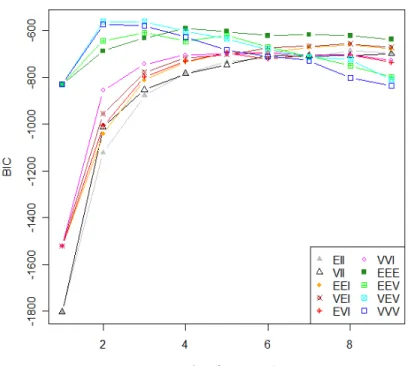
where the data is represented by x, πi is the probability that an observation belongs to distribution i and fi(x|µi,Σi) is the normal density of group i with mean µi and variance-covariance Σi. The parameters are estimated by Expectation-Maximization (EM) algorithm and the object is assigned to the component with maximum probability. The final compo-nents will be the clusters. In this way, the estimated probabilities of assignment of an object to a component can show if one object is highly correlated to more than one cluster, as in fuzzy clustering. In MCLUST, the normal distribution clustering modeling decomposes the variance-covariance matrix Σi in a set of geometric features that provide information about volume, shape and orientation of the components or clusters. Different parameteri-zations of the covariance matrix generate different models that are compared through the Bayesian information criterion (BIC) of Schwarz[88]. The best model is considered the one with maximum BIC over all models and numbers of components considered. Figure 2.4 shows a typical graph produced with MCLUST for different covariance parameterizations and different number of components6.
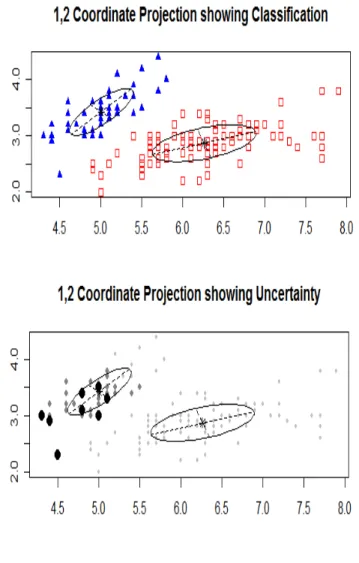
The assignment of probabilities to components in MCLUST also helps to produce graph-ical outputs, as projected clusters and projected degree of uncertainty in the allocation of objects to clusters. Figure 2.5 has examples of such graphs.
As observed by Fraley and Raftery [30], model-based clustering has also many drawbacks. The assumption that the dataset fits a specific distribution is not always accepted and may be difficult to justify in microarray or high dimensional data analysis. Also, the EM computations can fail when the covariance matrix of one or more components is singular or nearly singular, or yet, if the clusters contain few observations.
Model-based clustering using mixture of distributions has been largely studied with many applications to high-dimensional and microarray data. Examples are Fraley [28], McLachlan
Figure 2.4. BIC comparison of different models with different number of components in clustering of a data. The covariance structures considered are EII (spherical with equal variance), VII (spherical unconstrained), EEI (diagonal with equal variance), VEI (diagonal with equal shape), EVI (diag-onal with equal volume) , VVI (diag(diag-onal unconstrained), EEE (ellipsoidal with equal variance), EEV (ellipsoidal with equal volume and shape), VEV (ellipsoidal with equal shape) and VVV (ellipsoidal unconstrained). The best model is VEV with 2 clusters.
and Peel [65], McLachlan et al. [67], Fraley and Raftery [29], McLachlan et al. [66], Gan et al. [34], Gottardo et al. [38] and Gottardo et al. [39]7.
In comparison with other methods, MCLUST shows superior results when consider-ing clusters with symmetric distributions and a larger number of replications. However, MCLUST has poor results for simulated clusters with asymmetric distributions, since it is based on the assumption of having a mixture of normally distributed clusters. In all
Figure 2.5. Example of coordinate projections of clustered objects showing clustering (named as classification) and uncertainty of allocation.
simulations presented in this thesis, MCLUST was less efficient than PPCLUST.
In terms of clustering genes in microarray data, ANOVA methods have been used to declare genes as differentially expressed or not. In this thesis, all the clustering methods are based on similarity measures that come from p-values obtained from hypothesis test-ing in ANOVA specially developed under the setttest-ing of large number of factor levels and small sample sizes. The next subsection gives a brief review of the use of ANOVA in gene
expression studies.
2.2.5
ANOVA methods in clustering analysis
ANOVA methods (see Pavlidis [78], Kerr et al. [53], Milliken et al. [71]) have been pro-posed to determine which genes are differentially expressed over samples obtained under different experimental conditions or across different kinds of tissue samples. However, few studies have been concerned with the use of ANOVA methods when the number of genes is large and the number of observations is small. Usually the application of ANOVA meth-ods for discovering differentially expressed genes in replicated microarray data is reduced to the identification of just two categories, expressed and non-expressed genes through the comparison of the expression of pairs of genes (Pan [75], Pavlidis et al. [78], and Sykacek et al. [101].). However, traditional ANOVA imposes strong assumptions that make it im-practical and not powerful enough. The assumptions include normality, independence and homocedasticity of errors. The assumption of normality of gene intensity distributions is difficult to justify in many microarray applications even after applying the common log transformation used in most studies. To solve this problem, authors use permutation tests or bootstrap methods, as in Kerr et al. [53], but then more replicates are required than are usually found in HDLSS or HDLLSS datasets as explained by Simon et. al [95]. Some other ANOVA methods with large numbers of factor levels are given in Boos and Brownie [14], [13], Akritas and Arnold [2], Akritas and Papadatos [3], and Wang and Akritas [112]8.
An-other assumption that requires attention is homocesdasticity. Dubin et al. [24] showed that usual log transformations are subject to problems such as not stabilizing data in microar-rays uniformly. Finally, multiple testing in ANOVA studies generate significance levels with extremely low p-values due to the high dimensionality of the problem and experimentwise Type I error rates are too conservative. In this situation it is frequently used in applications of false discovery error rate (FDR) by Benjamini and Hochberg [11]. FDR is defined as the 8All cited references are not concerned directly with microarray experiments, but with ANOVA when
expected proportion of false positives among the number of rejections. However, methods using FDR are still restricted to a gene by gene analysis and cannot borrow information from other genes.
The use of non-parametric methods may correct many of the problems mentioned above, but in many cases it results in a loss of power and if, still requires some assumptions to be valid as mentioned by Mehta et al. [69] and Roy [86].
In this thesis, two specific nonparametric hypothesis tests of no group effect are used in presence of a large number of factors levels when the number of observations is small. In this case, the p-values from the tests can be used as similarity measures in algorithms for clustering. Chapter 3 introduces the test used for clustering HDLSS data and a novel partitioning algorithm that has many advantages over existing algorithms in the literature. In Chapter 5, the developed algorithm is evaluated through numerical comparisons and applied to a microarray data. In Chapter 6a new test is developed for simple effects in high dimensional low sample size data in longitudinal studies. The asymptotic distributions of the test statistics are derived. Simulation studies concerning Type I error rates and power estimates of the new test are reported. This new test is used for implementation of the clustering algorithm that allows clustering of a large number of variables when only few replications over time are available. Finally, Chapter 7 presents conclusions about results obtained and discusses future research possibilities and perspectives. Each chapter identifies important references in the recent literature, but the reference list is not exhaustive due to the huge and even daily amount of new publications in this area.
Comment:
Other algorithms for clustering replicated microarray gene expression data have been used for specific situations with relative success. Examples: gene-shaving (Hastie et al. [42], and K-A. Do et al. [23]), density-based hierarchical clustering (Jiang et al. [48]), clustering via iterative feature filtering or CLIFF (Xing and Karp [116]), plaid models (Lazzeroni and Owen [60]), subspace clustering (Parsons et al. [77]), and coupled two-way clustering
analysis of gene microarray data (Getz et al. [37]). However, comparisons by simulation using those methods were not possible for the following reasons: lack of flexibility to do the simulations (no code access), poor documentation or/and incompatibility with different operational system platforms and versions of statistical packages.
2.3
Cluster Quality by Adjusted Rand Index
The Adjusted Rand Index (ARI) from Hubert and Arabie [46] is a measure of agreement in order to compare clustering results against an external criteria. An external criteria is some standard result for clustering that is judged to be correct, or even the result of clustering with a different methodology that someone wants to compare with other methods.
Consider, for example, a partition P1 ={rc1, rc2, . . . , rck} representing k reference clus-ters that will be used to compare clustering procedures. Let P2 = {oc1, oc2, . . . , occ} be a partition of c clusters obtained from some clustering algorithm (k-means, som, etc.). The Contingency Table9 2.1, represents the results of both clustering procedures, where n
ij is the number of objects that are in both clusters rci and ocj, with i = 1, . . . , k, j = 1, . . . , c, and ni.=
Pc
j=1nij, n.j =
Pk
i=1nij.
Table 2.1. Contingency Table of clustering agreement.
oc1 oc2 . . . occ rc1 n11 n12 . . . n1c n1. rc2 n21 n22 . . . n2c n2. .. . ... ... ... ... ... rck nk1 nk2 . . . nkc nk. n.1 n.2 . . . n.c n
Using this notation, the ARI can be calculated as, P i P j nij 2 − P i ni. 2 P j n.j 2 / n 2 1 2 P i ni. 2 + P j n.j 2 − P i ni. 2 P j n.j 2 / n 2 . (2.7)
ARI = 1, if the partitions agree completely, regardless of the permutation of the labels, or equivalently, if all elements in the same cluster in one partition are also together in some cluster in the other partition, for all clusters in both partitions. ARI = 0 when the elements in each partition are randomly assigned to each cluster. As an example, consider Table 2.2 with results from a clustering algorithm that is supposed to cluster 2000 objects in groups of sizes 200, 200, 800, 400, and 400 (reference clusters). The result obtained in Table 2.2 results in ARI = 0.93123.
Table 2.2. Contingency Table of clustering agreement of2000 clustered objects.
1 2 3 4 5 6 Total 1 0 6 182 7 4 1 200 2 0 3 1 0 0 192 200 3 6 791 2 0 0 1 800 4 2 2 0 0 396 0 400 5 0 19 0 375 2 4 400 Total 8 821 185 382 402 202 2000
A SASc macro to calculate ARI was implemented for SASc Version 9.1.3 and used in our simulations. The macro was adapted from Fisher and Hoffman [27] and corrected for the latest version of SASc language10. R software has ARI implemented in package
MCLUST.
3
Partition Clustering of HDLSS Data
Based on
p-Values
This chapter introduces a computational algorithm for partition clustering of a large number of variables with few observations per variable 1. The algorithm uses the one-way ANOVA model based on ranks developed by Wang and Akritas [112]. Clustering of High Dimensional Low Sample Size (HDLSS) data has been extensively used in the analysis of replicated data represented by a mixture of unknown distributions where individuals from a cluster are all generated from the same distribution. However, existing clustering algorithms applied to HDLSS data suffer from several drawbacks as noted in Chapter 2. The algorithm introduced in this thesis does not suffer from such drawbacks. Additionally, the new algorithm has better performance in finding the correct groups of factor levels (variables).
The new procedure, based on ANOVA methods, uses the p-value of the test statistic from Wang and Akritas [112] as a measure of similarity between groups. Classical ANOVA models and ANOVA based on ranks have been used in many studies with high dimensional 1For simplicity of description, we refer to a variable as a level of a factor. For example, different genes
data. See Brownie and Boos [14], Kerr et al. [53] and Wu et al. [115] for examples.
In HDLSS data problems, differences among factor levels can be reflected in many dif-ferent ways. The observations from difdif-ferent factors may have difdif-ferent mean values or the replicated data may have different variances. In this thesis, the problem of clustering on ob-servations from all factor levels is stated as the problem of detecting a significant difference on the distribution of the observations from each factor level. Let Xij denote thejth obser-vation from the ith factor level where {X
ij,1≤ j ≤ ni} are independent observations from some unknown distribution Fi(x), i = 1,2, . . . , a. We first test to see if these observations are from the same distribution, that we test
H0 :F1(x) =. . .=Fa(x). (3.1) Classical ANOVA tests whether the means of observations from each factor level are the same. However, these methods require error terms to be i.i.d. normal and with a constant variance (homocedasticity). The Kruskal-Wallis test can be used where the data are not normal by computing th usual analysis of variance test statistic from the ranks, rather than on the original observations. This test can be applied when the number of treatments is small; but the test is not valid in a high dimensional setting since the inference is based on large sample size and small number of distributions. Akritas and Arnold [2] showed that the ANOVA F test is robust to departure from homocedasticity when there is a large number of factors, but it is not asymptotically valid for unbalanced data with small sample sizes, even under homocedasticity. Later, Akritas and Papadatos [3] considered test procedures for unbalanced and/or heterocedastic situations when the number of factors tends to infinity. However, their test still requires that the number of replications goes to infinity suitably fast. Finally, trying to solve all such limitations, Wang and Akritas [112] considered a nonparametric rank test of the null hypothesis of equality of distribution functions for each factor level when the number of factors is large and the number of replications is either small2
or large. The use of Wang and Akritas [112] procedure in the new clustering algorithm gives 2This is the situation defined here as HDLSS data.
a large amount of flexibility considering balanced and unbalanced data, homocedastic or heterocedastic cases, small or large sample sizes and non-normality of error terms.
3.1
The Nonparametric Test of No Group Effect
This section explains the nonparametric test that allows one to detect the effect of the group factor by considering a large number of factor levels simultaneously. The p-value produced from such a test provides a measure of homogeneity among the levels considered in the test. First, let Xij denote the jth observation from theith factor, where{Xij,1≤j ≤ni}are independent observations from some unknown distributionFi(x),i= 1,2, . . . , a. When the distributions from all factor levels are the same, all observations are i.i.d. realizations of a common distribution. A matrix of elements Xij with rows representing factors,i= 1, . . . , a, and columns representing observations (replications), j = 1, . . . , ni is shown in Table3.1.
Table 3.1. High dimensional data layout, where a→ ∞ and ni ≥2. Factor Level Observations Sample size
1 X11 X12 . . . X1n1 n1
2 X21 X22 . . . X2n2 n2
..
. ... ... ... ... ...
a Xr1 Xr2 . . . Xrnr na
LetRijrepresent the rank of observationXij in the set of alln1+n2+. . .+naobservations. Then, under H0, these ranks are discrete uniformly distributed random numbers between 1 and Pa
i=1ni. Now, define the test statistic,
FR=
M STR
M SER
(3.2)
where M STR is the mean square error due to factor levels, calculated over ranks. That is,
M STR= 1 a−1 a X i=1 ( ¯Ri.−R˜..)2, (3.3)
and M SER is the estimate of sample variance, also obtained over ranks, or M SER= 1 a a X i=1 1 ni SR,i2 . (3.4) Note that ¯Ri. = n−i 1 Pni
j=1Rij is the mean rank of each factor level, ˜R.. = a
−1Pa
i=1R¯i. is the overall mean of factor levels, and S2
R,i is the sample variance calculated for each factor. The following theorem, by Wang and Akritas [112], uses the test statistic defined in (3.1) to give the asymptotic distribution of √a(FR−1) underH0 in HDLSS data where FRis the test statistic defined in (3.2).
Theorem 3.1. Let H0 : F1(x) = . . . =Fa(x) be satisfied, with Fi(x) arbitrary . If ni ≥ 2 fixed, assuming the observations are independent, the following limits exist
v22 = lim a→∞ 1 a a X i=1 1 ni σi2 >0 and τ2 = lim a→∞ 1 a a X i=1 2σ4 i ni(ni−1) . Then, as a→ ∞, √ a(FR−1) d →N(0, τ2/v24). (3.5) The statistic√a(FR−1) can be used to obtain ap-value for the test and compare it with some specified significance level α, such that the p-value works as a similarity measure in the algorithm. In this way, large p-values indicate the factor levels being tested are similar in distribution, and factors levels belong to the same group. In contrast, a small p-value gives evidence against H0 indicating that at least two groups of factors are required.
The performance of the test is verified here through analysis of Type I error rates in simulated data.
3.1.1
Type I Error Rate
Wang and Akritas [112] reported simulation studies in two-way ANOVA showing that their test statistic has a stable Type I error rate and the test works even when the error distri-bution is not normal. A numerical study on performance of the test statistic under the one
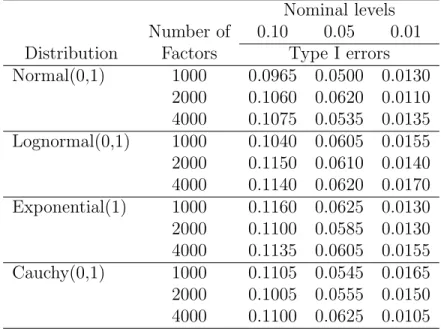
way model has not been reported in literature. Table 3.2 reports the approximate Type I error rates using the asymptotic distribution of the test statistic in 3.5 at levels 0.10, 0.05 and 0.01. For performance of other nonparmetric tests in such a setting, one should see Akritas and Papadatos [3]. In the simulations a takes on the values 1000, 2000 and 4000, and the number of observations per factor level is set to 4. The simulations are based on 2000 replications and observations were generated from normal, lognormal, exponential, and Cauchy distributions. The jackknife estimators3 of σ4
i were used in the estimation of the asymptotic variances from (3.5).
Table 3.2. Estimated levels for one-way ANOVA Nominal levels Number of 0.10 0.05 0.01 Distribution Factors Type I errors Normal(0,1) 1000 0.0965 0.0500 0.0130 2000 0.1060 0.0620 0.0110 4000 0.1075 0.0535 0.0135 Lognormal(0,1) 1000 0.1040 0.0605 0.0155 2000 0.1150 0.0610 0.0140 4000 0.1140 0.0620 0.0170 Exponential(1) 1000 0.1160 0.0625 0.0130 2000 0.1100 0.0585 0.0130 4000 0.1135 0.0605 0.0155 Cauchy(0,1) 1000 0.1105 0.0545 0.0165 2000 0.1005 0.0555 0.0150 4000 0.1100 0.0625 0.0105
The Type I error rates reported in Table 3.2 are close to the true α levels, indicating that the test statistic √a(Fr−1) performs well in testing the hypothesis in (3.1) regardless
3