*Correspondence to: Izhak Rubin, Department of Electrical Engineering, University of California, Los Angeles (UCLA), Los Angeles, California 90095, U.S.A.
Contract/grant sponsor: UC MICRO/SBC Paci"c Bell; contract/grant number: 98-131 Contract/grant sponsor: ARO; contract/grant number: DAAGIJ-98-1-0338
Received 1 February 2000
Department of Electrical Engineering, University of California, Los Angeles (UCLA), Los Angeles, California 90095, U.S.A.
SUMMARY
We present a multiplicative multifractal process to model tra$c which exhibits long-range dependence. Using tra$c trace data captured by Bellcore from operations across local and wide area networks, we examine the interarrival time series and the packet length sequences. We also model the frame size sequences of VBR video tra$c process. We prove a number of properties of multiplicative multifractal processes that are most relevant to their use as tra$c models. In particular, we show these processes to characterize e!ectively the long-range dependence properties of the measured processes. Furthermore, we consider a single server queueing system which is loaded, on one hand, by the measured processes, and, on the other hand, by our multifractal processes (the latter forming a MF
/MF/1 queueing system model). In comparing the performance of both systems, we demonstrate our models to e!ectively track the behaviour exhibited by the system driven by the actual tra$c processes. We show the multiplicative multifractal process to be easy to construct. Through parametric dependence on one or two parameters, this model can be calibrated to"t the measured data. We also show that in simulating the packet loss probability, our multifractal tra$c model provides a better"t than that obtained by using a fractional Brownian motion model. Copyright 2001 John Wiley & Sons, Ltd.
KEY WORDS: performance modelling; multiplicative multifractal; network tra$c; analytic analysis
1. INTRODUCTION
Recent analysis of high-quality tra$c measurements have revealed the prevalence of
long-range-dependent (LRD) (or self-similar) features in tra$c processes loading packet switching
communications networks. Included are local area networks (LANs) [1], wide area networks
(WANs) [2], variable-bit-rate (VBR) video tra$c [3,4], and world wide web (WWW) tra$c [5].
These"ndings have greatly challenged the commonly assumed models for network tra$c; e.g.
RThis is available at ftp.bellcore.com under the directory/pub/world/wel/lan
}tra$c and /pub/vbr.video.trace, respectively. time scales, while a Poisson or Markovian process, which displays short-range dependence, exhibit burstiness over much shorter time scales. As a result, Poisson or Markovian models tend to yield overly optimistic performance predictions.
Recent modelling works have therefore focused on obtaining parsimonious models capable of
capturing the basic LRD property of tra$c processes. Such approaches include chaotic maps [6],
a LRD ON/OFF model [7], Cox's M/G/Rtype models [8}11], the fractional Brownian motion
(FBm) model [12,13], fractional autoregressive integrated moving-average (FARIMA) models [1,14], point processes [15], and pseudo models [16,17]. An issue of much interest is whether and
how multifractal can be employed to model LRD tra$c. Recently, Taqqu et al. [18] have
analysed aggregated network tra$c processes using the multifractal concept. They conclude that
when self-similar tra$c models can be applied, multifractal models may not be needed.
The concept of multifractal is mostly developed in understanding the intermittent features of
turbulence [19]. Intermittency, when paraphrased to a meaning appropriate for network tra$c,
is a combination of burstiness of tra$c and the variation of the burstiness over time. Hence, it is conceivable that a simple multifractal model would su$ce to capture the basic (and possibly time
varying) bursty features of LRD tra$c. In this paper, we show that, based on a multiplicative
process structure, two simple multifractals, one used to model interarrival time series, and the other used for packet size sequences, each characterized by only one or two parameters, can be
readily constructed based on analysis of the measured tra$c trace data. We show that these
models provide excellent descriptions for LAN, WAN, and VBR video tra$c processes.
We have chosen Bellcore's Ethernet tra$c data and VBR video tra$c dataR for use in this
study. Four Ethernet data sets, denoted as pAug.TL, pOct.TL, OctExt.TL, and OctExt4.TL, and a VBR video data, denoted as MPEG.data, have been made available. Each Ethernet data set contains 1 million points representing measured values for arrival time stamps and packet sizes. Two Ethernet data sets (pAug.TL and pOct.TL) were measured on the&purple cable', involving
LAN tra$c. Another two Ethernet sets (OctExt.TL and OctExt4.TL) were collected on Bellcore's
link to the outside world, and have been classi"ed as WAN tra$c [18]. These sets cover time spans of 3142.8, 1759.6, 122797.8, and 75943.1 s, respectively. The video data consists of 174136 integers, representing the number of bits per video frame (24 frames/s for approximately 2 h). For
the study presented in this paper, we select a LAN tra$c set (pAug.TL), a WAN tra$c set
(OctExt.TL), and the video tra$c data (MPEG.data). We examine the interarrival time series
(which is deterministic for the video tra$c involving frame units) and the packet length sequences
derived from these data sets. We show the multiplicative multifractal processes to e!ectively
characterize the long-range dependence properties of these processes.
The remaining of the paper is organized as follows. In Section 2, after overviewing the de"nition of self-similar stochastic processes, we show that the interarrival time series and the packet length sequences derived from Bellcore's LAN and WAN tra$c trace data are self-similar. We then describe in Section 3 a class of multifractals, namely, random multiplicative processes.
To ease construction of multifractal models from measured tra$c trace data, we prove a number
of properties of multiplicative processes, and demonstrate that multiplicative processes can possess self-similar properties. We proceed in Section 4 with a detailed analysis of Bellcore's LA N,
WAN, and video tra$c data. We show that the interarrival time series and the packet length
2. SELF-SIMILAR INTERARRIVAL TIME SERIES AND PACKET LENGTH SEQUENCES OF NETWORK TRAFFIC
In this section, we overview the de"nition of second order self-similar processes, for the purpose of showing that the interarrival time series and the packet length sequences derived from Bellcore's
LAN and WAN tra$c trace data are self-similar. These descriptions also serve us in a later
section where we show multifractals to exhibit self-similar properties. The following de"nitions follow those made by Lelandet al. [1] and Beranet al. [3].
Let X"X
G: i"0, 1, 2,2 be a covariance stationary stochastic process with mean , varianceand autocorrelation functionr(k),k*0. Assumer(k) to be of the form
r(k)&k\@, askPR (1)
where 0((1. Note that
Ir(k)"R. This is referred to as the LRD property.
In characterizing the self-similarity of such processes, the most important parameter identi"ed is the Hurst parameterH. It is equivalent to, 1/2(H"1!/2(1. The value ofHmeasures
the degree of persistence of the correlation: the larger the H value, the more persistent the
correlation is.
For eachm"1, 2, 3,2, letXK"XK
G :i"1, 2, 3,2denote the new covariance stationary time series obtained by averaging the original seriesXover non-overlapping blocks of sizem, i.e.
XK G "(X
GK\K>#2#X
GK)/m, i*1 (2)
Self-similarity for X means that the processXK exhibits (exactly or asymptotically) the same
second-order statistics as those characterizing the processX.
A n e$cient method used to detect the self-similarity character of a stochastic process employs the variance-time relation [1]: Var(XK)&m\@. Thus, in plotting the variance of XK vs the aggregating block sizemon a log}log scale, we expect self-similar processes to yield a curve which tends to become linear for largem, having a slope larger than!1. By contrast, for a short-range-dependent process, we have Var(XK)&m\.
Two random processes, the interarrival time series,¹
G, where¹
Gdenote theith interarrival
time between two successive packet arrivals, and the packet length sequences, BG, where BG
represents the length of theith packet, are used to de"ne a tra$c process. Two other random counting processes can be derived from these two time series. The latter processes represent the
number of packets and the number of bytes arriving during successive periods each of lengtht
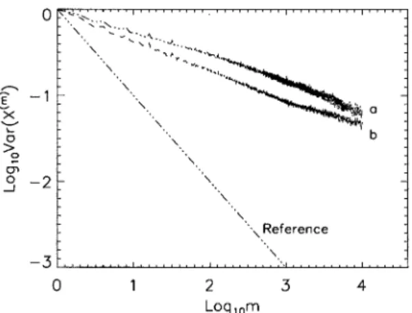
Figure 1. Variance}time plots (in logarithmic scale) for interarrival time series ¹
G and packet size
sequencesB
Gfor tra$c traces (a) pAug.TL, and (b) OctExt. The line denoted as&Reference'has slope!1.
Following Lelandet al. [1], self-similarity has been detected focusing on the analysis of these
counting processes. In contrast, we study in this paper the processes¹
GandBG. Using the
tra$c measurements mentioned in Section 1, we show these processes to be self-similar. This is
demonstrated by the results shown in Figure 1. We will furthermore show in this paper that
simple multifractal models for the¹
GandBGsequences can be readily constructed. Note that
¹
G"1/24 s, for the video tra$c.
3. MULTIPLICATIVE MULTIFRACTALS
In this section, we "rst overview the de"nition of multifractals. Multifractals are typically constructed through multiplicative processes. In the following, we de"ne multiplicative processes and present examples of such models. We then prove a number of properties of such processes that are most relevant to their use as network tra$c models.
3.1. Dexnition
Consider a unit interval. Associate it with a unit mass. Partition the unit interval into a series of small intervals, each of linear length. Also partition the unit mass into a series of weightswG,
and associatewGwith theith interval. Now consider the moments
MO()"
G wOG
(3) whereqis real. Note the convention that wheneverwHis zero, the termwOHis dropped. We also
note that a positiveqvalue emphasizes large weights, while a negativeqvalue emphasizes small
weights. If we have, for a real function(q) ofq,
MO()&OO asP0 (4)
for every q, and the weights wG are non-uniform, then the weights wG() are said to form
a multifractal measure. Note that the normalization
Figure 2. Aschematic illustrating the construction rule of a multiplicative multifractal.
Note that if wG are uniform, then (q) is linear in q. When wGare weakly non-uniform, visually(q) may still be approximately linear inq. The nonuniformity inwGis better character-ized by the so-called generalcharacter-ized dimensionsDOde"ned as [20]:
DO" (q)
q!1 (5)
DO is a monotonically decreasing function of q [21]. It exhibits a non-trivial dependence on
qwhen the weights wGare non-uniform.
3.2. Construction of multiplicative multifractals
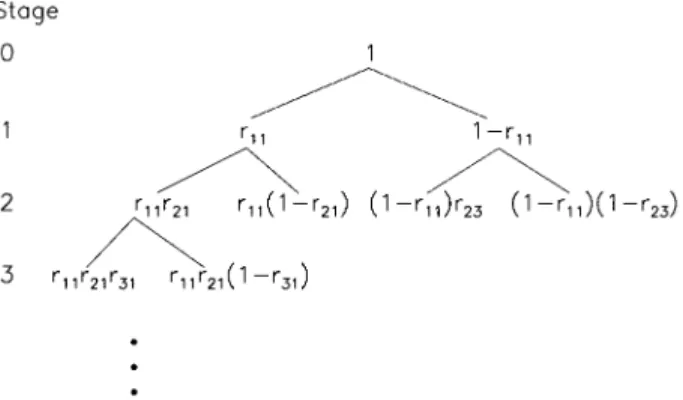
Consider a unit interval. Associate it with a unit mass. Divide the unit interval into two segments of equal length. Also partition the associated mass into two fractions,rand 1!r, and assign them
to the left and right segments, respectively. The parameter r is in general a random variable,
governed by a probability density function (pdf) P(r), 0)r)1. The fraction r is called the multiplier. Each new subinterval and its associated weight are further divided into two parts following the same rule. The procedure is schematically shown in Figure 2, where the multiplier
r is written asrGH, with i indicating the stage number. Note the scale (i.e. the interval length) associated with stageiis 2\G. We assume thatP(r) is symmetric aboutr"1/2, and has successive moments,,2. HencerGHand 1!r
GHboth have marginal distributionP(r). The weights at the
stageN,wL,n"1,2, 2,, can be expressed asw
L"u u2u
,, whereuJ,l"1,2,N, are either
rGHor 1!r
GH. Thus,uG,i*1are independent identically distributed random variables having pdf
P(r). In the following, we illustrate this process by selecting a speci"c pdfP(r).
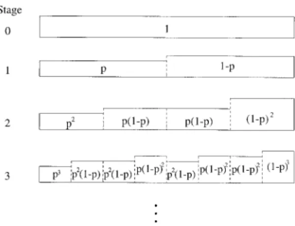
3.2.1. Deterministic binomial multiplicative process. In this case, the pdf is set to be equal to
P(r)" (r!p), where (x) is the Kronecker delta function. Thus,r"pwith probability 1, where 0(p(1 is a"xed number. The weights obtained for the"rst several stages are schematically shown in Figure 3.
Figure 3. Aschematic showing the weights at the"rst several stages of the binomial multiplicative process.
For this process, at stagen, we have
MO()" L
GCGLpOG(1
!p)OL\G"(pO#(1!p)O)L (6)
Since at stagen,"2\L, we obtain
(q)"!ln(pO#(1!p)O)/ln 2 (7) which is independent ofn(or). Hence, this weight process constitutes a multifractal.
3.2.2. Random binomial multiplicative process. To make the weight series random, we modify
P(r) to become
P(r)"( (r!p)# (r!(1!p)))/2, (8) so thatP(r"p)"P(r"1!p)"1/2. Hence,P(r) is symmetric aboutr"1/2. Arealization of the weights at stage 12 (withp"0.3) is shown in Figure 4(a).
3.2.3. Random multiplicative process. The functionP(r) can be selected to follow any functional form [21]. The following piece-wise linearP(r) function is used to generate the weight realization (at stage 12) shown in Figure 4(b):
P(r)"
2r#0.5 if 0)r)0.5
Figure 4. Weight series at stage 12 for (a) the modified binomial multiplicative process (p"0.3), and (b) the random multiplicative process with the multiplier pdf given in the text.
3.3. Properties of multiplicative multifractals
For the weights at stageN, we prove the following properties to hold.
(i) MO()&OO, with"2\,,(q)"!ln(2
O)/ln 2. This follows the observation that at stage N, MO()"E( ,
L(wL)O)"2,E(wO)"2,E((uu2u,)O)"2,,O. This property indicates that a multiplicative process is a multifractal, and relates the(q) spectrum to the moments of the multiplier distribution.
Note that forP(r)"[ (r!p)# (r!(1!p))]/2, we have
O"[pO#(1!p)O]/2. Hence, (q)"!ln[pO#(1!p)O]/ln 2. We thus note that the function(q) assumed by a random binomial process is the same as that exhibited by a deterministic binomial process (Equation (7)). This is expected to be the case since the value assumed byMO(), and thus also(q), is independent of the speci"c ordering of the weights.
(ii) E(w)"E(w
L)"E(u u2u
,)"2\,,n"1,2, 2,. (iii) Var(w)"Var(w
L)",
!2\,, n"1,2, 2,. To prove this relation, we note that
E(w)"E(w
L)"E((u u2u
,))", .
(iv) WhenN<1, the weights at stageNhave log-normal distribution. This is deduced directly by taking the logarithm ofwL"u
u2u
,.
(v) E[(wL!E(w))(w
L>K!E(w))]"(1/2!
),\(4)\I!2\,, form"2I, wherek is an
integer. Hence, the covariance function decays with time lagmin a power-law manner.
To prove assertion (v), we consider two weightswL
andwLat stageN. Assume they share
the same ancestor weight xat stageN!k, i.e.w
L"xrIJ\rJ, wL"x(1!r)IJ\rJ,
whererandrGJ,i"1, 2,l"1,2,k!1are independent random variables with distribu-tion P(r). Then E[(wL
!2\,)(wL!2\,)]"E(x)E[r(1!r)]E[IJ\rJrJ]!2\,"
2\I\,\I(1/2!
)!2\,. Form"2I, all pairs ofw
L, wL>K, forn*1, share an
ancestor at stage N!k!1. Hence, E[(w
L!E(w))(w L>K!E(w))]" 2\I,\I\(1/2! )!2\,"(1/2! ),\(4)\I!2\,. (vi) Var(=K)", (4)\I!2\,, where =K"(w GK\K>#2#w GK)/m, m"2I,
k"1, 2,2, andi*1. This is proven by expressing=K"2\Ix, wherexis a weight at stageN!k.
The equation in (vi) expresses a variance-time relation. For LRD tra$c [16],
processes, when N is large and '0, the term ,
(4)\I dominates. Hence, the functional variation of log Var(=K) vs logmis linear, with the resulting slope,!log(4
)/log 2, providing
an estimate of 2H!2. The linear property is demonstrated by Figure 5 which shows the
variance-time plots for the times series of Figure 4.
Also note that the dependence of Var(=K) on m is the same as that of
E[(wL!E(w))(w
L>K!E(w))] onm. Below we show that, by analysing measured tra$c processes, one can e!ectively model LRD tra$c by using multiplicative multifractals by properly selecting the multiplier distributionP(r).
4. MULTIPLICATIVE MULTIFRACTAL ANALYSIS OF LAN, WAN, AND VBR VIDEO TRAFFIC
Our purpose of multifractal analysis of network tra$c is to check whether the interarrival time
series¹
Gand packet length sequencesBGof the tra$c data can be viewed as realizations of multiplicative processes. If they are only approximately multifractals, an equivalent multifractal model may still be constructed. In this section, we show that the interarrival time series and packet length sequences of Bellcore's LAN and WAN tra$c data, and the frame size sequences of
the video tra$c data, exhibit stochastic features which are consistent with the stochastic
behaviour of random multiplicative processes.
There are two ways to check whether¹
GandBGare realizations of certain multiplicative
processes. One method is to compute the moments MO() at di!erent stages, and check
whether Equation (4) is valid for certainranges. Another method is to compute the multiplier
distributions at di!erent stages, and check whether they are stage independent. We note the
latter method to be typically more useful when constructing a multiplicative process for ¹
G
or BG. In the following, we describe in detail a general procedure for obtaining weight
sequences at di!erent stages needed for computing the moments MO() and the multiplier
distributions.
Assume there are 2,arrivals. For ease of illustration, we denote¹
GorBGbyXG. We view
XG,i"1,2, 2,as the weight series of a certain multiplicative process at stageN. Note that the
total weight ,
GXGis set equal to 1 unit. Also note the scale associated with stageNis"2\,. This is the smallest time scale resolvable by the measured tra$c data.
Given the weight sequence at stageN (which represents the measured data), the weights at
stage N!1, X
G ,i"1,2, 2,\, is obtained by simply adding the consecutive weights at stageNover non-overlapping blocks of size 2, i.e.X
G "X
G\#X
G, fori"1,2, 2,\, where the superscript 2forX
G is used to indicate that the block size used for the involved summation
at stageN!1 is 21. Associated with this stage is the scale"2\,\. This procedure is carried out recursively. That is, given the weights at stagej#1,X,\H\
G ,i"1,2, 2H>, we obtain the weights at stage j, XG,\H, i"1,2, 2H, by adding consecutive weights at stage j#1 over non-overlapping blocks of size 2, i.e.
XG ,\H"X,\H\
G\ #X,\H\
G (9)
fori"1,2, 2H. Here the superscript 2,\HforX,\H
G is used to indicate that the weights at stage
jcan be equivalently obtained by adding consecutive weights at stageNover non-overlapping
Figure 5. Variance}time plots for the time series of Figure 3, (a) the modi"ed binomial multiplicative process, and (b) the random multiplicative process. The length for both time
series is 2. The line denoted as&Reference'has slope!1.
Figure 6. Aschematic showing the weights at the last several stages for the analysis procedure described in the text.
where we have a single unit weight, ,
GXG, and "2. The latter is the largest time scale
associated with the measured tra$c data. Figure 6 schematically shows this procedure.
After we have obtained all the weights from stages 0 toN, we compute the momentsMO()
according to Equation (3) for di!erent values ofq. We then plot logMO() vs logfor di!erent values ofq. If these curves are linear over wide ranges of, then these weights are consistent with a multifractal measure. Note that, according to Equation (4), the slopes of the linear part of logMO() vs logcurves provide an estimate of (q), for di!erent values ofq.
Next, we explain how to compute the multiplier distributions at di!erent stages. From stage
jtoj#1, the multipliers are de"ned by the following equation, based on Equation (9):
rGH"X
,\H\
G\
XG ,\H (10)
fori"1,2, 2H. We view rH
G , i"1,2, 2Has sampling points of the multiplier distribution at stage j,PH"P
H(r), 0)r)1. Hence P
H can be determined from its histrogram based onrGH, i"1,2, 2H. We then plot P
Figure 7. log
MO() vs!log
for ¹
GandBG
of pAug.TL for several di!erentq's.
Figure 8. log
MO() vs!log
for ¹
GandBG
of OctExt.TL for several di!erentq's.
together so thatPH&P, then the multiplier distributions are stage independent, and the weights
form a multifractal measureP.
We illustrate the above procedure by analysing Bellcore's tra$c trace data pAug.TL,
OctExt.TL, and MPEG.data. We use the"rst 2arrivals of the Ethernet trace data, and the"rst 2video frame size data for this analysis. Figures 7, 8 and 10(a) show logMO() vs!log
for
processes¹
GandBGof pAug.TL and OctExt.TL, and the frame size sequences of the video
tra$c data, respectively. We observe that the scaling between MO() and (i.e. the degree of linearity between logMO() and!log
) forBGof the Ethernet data sets are excellent. While
the scaling betweenMO() andfor¹
Gof the Ethernet data and the frame size sequences of the
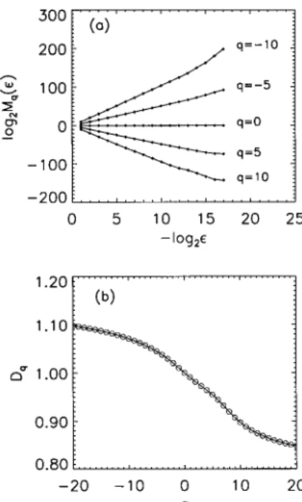
video tra$c is slightly worse, yet it is still quite good. To further check whether these data sets are truly multifractals, we computeDO. These results are shown in Figure 9, for the Ethernet data, and Figure 10(b), for the frame size sequences of the video tra$c. Indeed we observe that in all casesDO has a nontrivial dependence onq. Therefore, we conclude that these time series are consistent with multifractals.
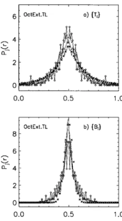
Next we compute the multiplier distributions at di!erent stages for¹GandBGof pAug.TL and OctExt.TL. Figure 11 shows, for pAug.TL, the multiplier distributionsPHfor¹
GandBGat
di!erent stagesj. Plotted in Figure 11(a) is an asteroid curveP(r)&\?P\, with"8, where subscript e designates the double exponential pro"le ofP(r). Collapsed on it are"veP
Hcurves with j"11,2, 15. Also shown isP
Hwithj"9 as a diamond curve, which is observed to deviate from the asteroid curve. Note that if we"t it with a double exponential curve, thenhas a value larger than 8. In fact,increases monotonically with the decrease of the stage numberjwhenj)11. As
Figure 9. The generalized dimension spectrum for
¹
GandBGof (a) pAug.TL, and (b) OctExt.TL.
Figure 10. (a) log
MO() vs !log
, and (b) the generalized dimension spectrum for the frame size
sequence data MPEG.data.
will be discussed in the next section, taking this into proper consideration is of key importance to a successful modelling.
Next, we consider theBGprocess for pAug.TL. This is shown in Figure 11(b). The asteroid
curve is generated from P(r)&e\?P\, with "80, where subscript g designates the Gaussian shape ofP(r). Collapsed on it are threePHcurves withj"9, 10 and 11. Also shown is a diamond curve forPHwithj"8. Again, if we"t a Gaussian-shaped curve to thisP
H, then the
value foris larger than 80. Note thatalso monotonically increases with the decrease of the
stage numberjwhenj)9. Thus we conclude that for pAug.TL, bothB
Gand¹
Gprocesses are
multifractals in a certain time scale range.
The results for OctExt.TL are shown in Figure 12, where asteroid curves are generated from
P(r)&e\?P\, with"7 andP(r)&e\?P\with"270 for¹
G(Figure 12(a)) andBG
(Figure 12(b)), respectively. Collapsed on them arePHcurves withj"11, 12 and 13 for¹
G, and j"9, 10 and 11 forB
G. Also plotted as diamond curves arePHwithj"8 for¹
G, andPHwith j"7 forB
G. Note that if we"t a double exponential curve toPHwithj"8 for¹G, thenis
larger than 7. However, nowno longer increases monotonically with the decrease of the stage
numberj. We thus note a distinctive di!erence between the data collected for LAN and WAN
tra$c. This will be further discussed in the next section. For theBGsequence of OctExt.TL, if we "t a Gaussian-shaped curve toPHwithj"7 forBG, thenis much smaller than 270, and
Figure 11. Multiplier distributionsP
Hfor (a)¹
G,
and (b) B
G of pAug.TL. See the text for moredetail.
Figure 12. Multiplier distributionsP
Hfor (a)¹
G,
and (b)B
Gof OctExt.TL. See the text for moredetail.
BGprocess of pAug.TL,increases monotonically with the decrease of the stage numberj. The consequence of this di!erence will be further discussed in the next section.
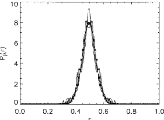
The result for MPEG.data is shown in Figure 13, where the asteroid curve is generated from
P(r)&e\?P\, with"200. Collapsed on it areP
Hcurves withj"8,2, 11. Again we see that the frame size sequences of the video tra$c form a multifractal process over certain time scales. We have observed an interesting feature that the weights at those particular stages where they form a multiplicative process follow approximately log-normal distribution. This is consistent with property (iv) of Section 3.3.
In summary, we have shown that theBGand¹
Gsequences for the pAug.TL and OctExt.TL
data sets, and the frame size sequences of MPEG.data, behave as multifractals over certain time scale ranges. The behavior of the process outside the latter time scale is not governed by a multiplicative multifractal process. Nevertheless, we can approximate its behaviour by still using a multifractal model, as illustrated in the next section.
5. MF/MF/1 QUEUEING SYSTEM
In this section, we consider a MF/MF/1 queueing system, where MF and MF denote
multifractal interarrival time series and packet size sequences with appropriate parameters. We
Figure 13. Multiplier distributionsP
Hfor the frame size sequence data MPEG.data.
See the text for more detail.
matches that obtained when the queueing system is driven by the actual tra$c processes.
Furthermore, this has been noted to be the case for all examined LAN, WAN, as well as VBR video tra$c processes. Let us brie#y recapitulate the procedure for constructing a multiplicative process.
Assume that over the observation period of the tra$c process, there are 2,arrivals, with mean interarrival time and mean packet length given by¹andb, respectively. The observation time is
thus equal to ,
G¹G"2,¹, while the total length of the packets is ,
GBG"2,b, where¹
Gand BGdenote theith interarrival time and packet length, respectively. We view 2,¹and 2,bas the weights at stage zero of the interarrival and packet-length multiplicative processes, respectively. Assume the multiplier distribution is already chosen (this will be discussed shortly). Then, we can follow the standard procedure described in Section 3.2, to construct the 2,samples¹
GandBG
at stageNfor the two modelled processes.
Assume a single server queueing system using a FIFO service discipline and an in"nite bu!er, with interarrival times and packet sizes modelled by random multiplicative processes, as
de-scribed above. Denote such a queueing system by MF/MF/1, where subscripts e and g designate
the multiplier distributions P(r) to be double exponential (P(r)&e\?P\) and Gaussian (P(r)&e\?P\) characterized by parameters and , respectively. Thus our multifractal tra$c model contains four parameters:,, the mean interarrival time¹, and the mean packet lengthb. Our purpose is to"nd proper values forandto model the actual tra$c trace data.
For this purpose, we simulate a MF/MF/1 queueing system and compare its behaviour
(through observation of the system size tail distribution) to a queueing system driven by the
actual tra$c trace. We then select values forandso that the latter two queueing systems
exhibit similar performance under several loading ratio conditions.
Here again, we use the"rst 2arrivals of the Ethernet tra$c trace data. For modelling the
video tra$c, we use the whole sequence (of length 174136) of the frame size data. Since
2(174136(2, we generate a multiplicative process till stage 18 and retain the"rst 174136 weights at stage 18. We then rescale them so that their average is equal to the mean of the observed frame sizes.
AssumingP(r)&e\?P\ or &e\?P\, then P(r)P (r!1/2) when
or PR. The
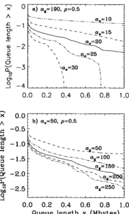
Figure 14. Complementary queue length distributions of MF
/MF/1 queueing systems with (a)"0.5,
"190, and 5 di!erent
's; and (b)"0.5,
"50, and 5 di!erent
's. The mean interarrival time and mean packet length are the same as those for pAug.TL.
processes. This leads us to expect that given the mean interarrival time and the mean packet length, the burstiness of the tra$c monotonically increases with the decrease of(or). Figure
14(a) shows the complementary queue length distributions when is"xed to be 190 and the
utilization is set equal to"0.5. The"ve illustrated curves, from top to bottom, correspond to
"10, 15, 20, 25 and 30. The results for a"xed value of
"50 and"0.5 is shown in Figure 14(b), where "ve curves, from top to bottom, correspond to "50, 100, 150, 200 and 250, respectively. These results clearly con"rm the above-mentioned property, illustrating the mono-tonic increase in the burstiness of the tra$c processes resulting as we decrease theparameters.
We note an interesting feature exhibited by Figure 14(b). The burstiness of the tra$c decreases non-uniformly with the increase of: it decreases quite fast whenis small, and very little when is already large. We note that whenis already large, the burstiness contributed byis much smaller than that contributed by. Further increase ofwill not result in a signi"cant reduction in the burstiness of the tra$c. WhenPR, the burstiness of the tra$c is solely determined by. This observation is also valid whenis"xed andis varied.
The observed burstiness behaviour of the MF/MF/1 system is consistent with the properties
(iii), (v) and (vi) of Section 3.3. Larger values for and/or correspond to smaller second
momentum, hence, smaller variation.
We have simulated the queue-size behaviour of the MF/MF/1 system by selecting the
andvalues associated with the asteroid curves in Figures 11 and 12. We have found this model
to yield a system-size tail distribution which is longer than that obtained when pAug.TL is used to drive the queueing system, while it is shorter than that obtained when OctExt.TL is used to drive
Figure 15. Comparison of complementary queue length distributions of single server FIFO queueing systems driven by measured data (a) pAug.TL, (b) OctExt.TL, and (c) MPEG.data (dashed lines), and of corresponding MF
/MF/1 queueing systems (solid lines). The parameters used for the MF/MF/1 queue-ing systems are (a) (
,)"(20, 190), (b) (
,)"(6, 50), and (c) (
,)"(R, 150). Three curves, from top to bottom, correspond to"0.7, 0.5 and 0.3, respectively.
the queueing system. This is because the asteroid curves correspond to the estimated multiplier distributionsPHat quite large values ofj, corresponding to relatively short time scales. As pointed out in the last section, for pAug.TL, the and values "tted from PH at smaller values of
j(corresponding to longer time scales) are larger than those associated with the asteroid curves in Figure 11, while for OctExt.TL, theandvalues"tted fromPHat smaller values ofjare smaller than those associated with the asteroid curves in Figure 12. The results exhibited by Figure 14
indicate that the LAN tra$c process (pAug.TL) is less bursty for longer time scales than for
shorter time scales, while the WAN tra$c process (OctExt.TL) is more bursty for longer time
scales than for shorter time scales. By selecting theandvalues to be those associated with the
asteroid curves in Figures 11 and 12, the modelled tra$c processes exhibit the same degree of
burstiness at all time scales. This is the underlying reason that the MF/MF/1 system yields
a system-size performance behaviour which is not very close to that obtained when the measured
tra$c data, pAug.TL and OctExt.TL, are used to drive the queueing system.
Consequently, better values forandare selected by"tting the means ofP
Hover a multitude
of stages. To obtain a good"t of the system size tail distribution of a queueing system driven by the corresponding measured tra$c processes, we"nd (by trial and error) that for pAug.TL, (,
)"(20, 190), and for Oct.Ext.TL, (
,)"(6, 50). For the video frame size sequence data, the frame durations are"xed so that"R. We then"nd (also by trial and error) that"150. Note
that the value forfor the VBR video data is quite close to that associated with the asteroid
curve in Figure 13 ("180).
Figures 15(a)}(c) show a comparison of the complementary queue length distributions for
a queueing system loaded by the measured tra$c, pAug.TL, OctExt.TL, and MPEG. data, and
the corresponding MF/MF/1 queueing system models based on the above selected
dashed curves exhibit the results obtained from a queueing system driven by the measured tra$c
trace. The three curves in each "gure, from top to bottom, correspond to three
di!erent utilization levels,"0.7, 0.5 and 0.3. Using theandparameter values mentioned
above, the MF/MF/1 model proves to yield excellent "t of the complementary queue size
distributions of a queueing system loaded by the measured LAN, WAN, and VBR video tra$c.
6. COMPARISON BETWEEN THE MULTIFRACTAL TRAFFIC MODEL AND THE FBm MODEL FOR THE OBSERVED TRAFFIC PROCESSES
In this section, we make a comparison between the MF/MF/1 queueing system model and the
FBm model, as it relates to"tting the queue size tail distribution for a single server queueing
system loaded by the tra$c processes mentioned above.
FBm is the most intensively studied model exhibiting the long-range dependence property in tra$c engineering. After Norros [12, 13] introduced FBm as a tra$c model, Erramilliet al. [22] have checked the complementary queue length distribution formula of Norros [12,13], and found excellent agreement with simulations for a single server queueing system operated at utilization "0.5. By breaking their Ethernet tra$c into source}destination pairs, Willingeret al. [7] have shown that the long-range-dependent ON/OFF model is consistent with the data, and further proven that the ON/OFF model asymptotically approaches a FBm model. It has also been shown that analytic results similar to those exhibited by a single server queueing system driven by
a FBm tra$c process can be obtained for a queue fed by a tra$c process modelled by LRD
ON/OFF sources [23] and by a FARIMA model [14]. These works demonstrate the
e!ectiveness of the FBm model. In the following, we demonstrate, by considering measured LAN,
WAN, and VBR video tra$c data, that a multiplicative multifractal tra$c model can provide an
even better"t to the underlying complementary queue length distribution.
For this purpose, for the FBm model, we use the Norros'lower bound complementary queue
length distribution formula [12,13]:
P(<'x)&exp[!x\&] (11) with "m&\((1 !)/)& 2a
1!H H & # H 1!H \& (12)where the random variable < represents the (steady-state) un"nished load, H is the Hurst parameter,m'0 is the mean input rate,is the utilization level, andais a variance coe$cient. Using the measured tra$c trace data, we"rst estimate the parametersa[24] andH[1,3]; then we use Equation (11) to compute the complementary queue length distributions. We compare the computed queue length distributions with those obtained for a queueing system driven by the
measured tra$c trace data. Figure 16(a) shows the complementary queue length distributions for
pAug.TL for three di!erent utilization levels, "0.7, 0.5 and 0.3 (from top to bottom). The
dashed lines are from a queueing simulation with pAug.TL as input tra$c. The solid lines are
Figure 16. Comparison of complementary queue length distributions of single server FIFO queueing systems driven by measured data (a) pAug.TL, (b) OctExt.TL, and (c) MPEG.data (dashed lines), and corresponding FBm tra$c processes (solid lines). Three curves, from too to bottom, correspond to"0.7, 0.5 and 0.3, respectively. Note for MPEG.data, the solid curve for"0.3 is too close to they-axis to be seen.
then the solid line and the dashed line almost coincide, which is consistent with the result presented by Erramilliet al. [22]. Asalient feature exhibited by Figure 16(a) is that in terms of the complementary queue length distribution, given a certain utilization level (say, for example "0.5), by choosing theHvalue carefully, the FBm model can provide excellent"t. However, for
lighter and heavier loading conditions (smaller and largervalues), when the sameH value is
used, the model does not provide a good"t.
As is evident from Figure 16(c), this problem is also associated with the modelling of VBR video tra$c data.
The aforementioned problem can become even more pronounced when FBm is used to model
WAN tra$c. This is shown in Figure 16(b), where the solid curves are generated from Equation
(11), and the dashed lines are obtained from a queueing simulation with OctExt.TL as input tra$c. The exhibited three curves, from top to bottom, correspond to"0.7, 0.5 and 0.3.
In ATM networks, packet loss probability levels as small as 10\are of interest. Such low
probabilities lead to the almost vertically dropping segments of Figures 15 and 16. This feature is not predicted by Equation (11).
By comparing Figures 15 and 16, it is clear that the MF/MF/1 model has overcome both
problems. Hence, for the tra$c processes studied here, it yields more accurate results than the FBm model in predicting the behaviour of the complementary queue length distribution of the system (or equivalently, the packet loss probability).
7. CONCLUSIONS
We introduce a multiplicative multifractal process for the modelling of long-range-dependent
relevant to its use as network tra$c models. Through analysis of Bellcore's LAN, WAN and VBR video tra$c trace data, we show this process to provide excellent"t with measured tra$c data. The model employs two multifractals to characterize the self-similar interarrival time series and
the packet length sequence of the measured tra$c trace data, respectively. The multiplicative
model involves one to two basic parameters. Once the parameters are chosen, it is easy to construct. To calibrate the model, we have considered a single server queueing system which is loaded, on one hand, by the measured processes, and, on the other hand, by our multiplicative multifractal processes. In comparing the performance of both systems, we have demonstrated our
model to e!ectively track the behaviour exhibited by the system driven by the actual tra$c
processes. We have also shown that, for the measured tra$c processes studied here, our
multiplicative multifractal tra$c model provides more accurate results concerning the behaviour of the packet loss probability than those obtained using a FBm model.
ACKNOWLEDGEMENTS
Our thanks to the Bellcore researchers (Drs Leland and Garret) for making available their Ethernet tra$c trace data and the VBR video data. Without these data, this work would not be possible. J.B. Gao would also like to thank his friend Johnny Lin for teaching him LATEX. This work is supported by UC MICRO/SBC Paci"c Bell research grant 98-131 and by ARO grant DAAGIJ-98-1-0338.
REFERENCES
1. Leland WE, Taqqu MS, Willinger W, Wilson DV. On the self-similar nature of Ethernet tra$c (extended version).
IEEE/ACM¹ransactions on Networking1994;2:1}15.
2. Paxson V, Floyd S. Wide area tra$c*the failure of Poisson modeling.IEEE/ACM¹ransactions on Networking1995;
3:226}244.
3. Beran J, Sherman R, Taqqu MS, Willinger W. Long-range-dependence in variable-bit-rate video tra$c.IEEE
¹ransactions on Communications1995;43:1566}1579.
4. Garret MW, Willinger W. Analysis, modeling and generation of self-similar VBR video tra$c.Proceedings of ACM
SIGCOMM, London, England, 1994.
5. Crovella ME, Bestavros A. Self-similarity in world wide web tra$c: evidence and possible causes.IEEE/ACM
¹ransactions on Networking1997;5:835}846.
6. Erramilli A, Singh PR, Pruthi P. An application of deterministic chaotic maps to model packet tra$c.Queueing
Systems1995;20:171}206.
7. Willinger W, Taqqu MS, Sherman MS, Wilson DV. Self-similarity through high-variability: Statistical analysis of ethernet LAN tra$c at the source level.IEEE/ACM¹ransactions on Networking1997;5:71}86.
8. Cox DR. Long-range dependence: a review. InStatistics:An Appraisal, David HA, Davis HT (eds). The Iowa State University Press: Ames, IA, 1984; 55}74.
9. Likhanov N, Tsybakov B, Georganas ND. Analysis of an ATM bu!er with self-similar (&fractal') input tra$c.
Proceedings of IEEE InfoCom, Boston, MA, 1995.
10. Parulekar M, Markowski AM. Bu!er over#ow probabilities for a multiplexer with self-similar input.Proceedings of
IEEE InfoCom, San Francisco, CA, 1996.
11. Tsybakov B, Georganas ND. On self-similar tra$c in ATM queues: de"nitions, over#ow probability bound, and cell delay distribution.IEEE/ACM¹ransactions on Networking1997;5:397}409.
12. Norros I. Astorage model with self-similar input.Queueing Systems1994;16:387}396.
13. Norros I. On the use of fractional Brownian motion in the theory of connectionless networks.IEEE JSAC1995; 13:953}962.
14. Su YT. Personal communication, 1998.
15. Ryu B, Loven SB. Point process approaches for modeling and analysis of self-similar tra$c: Part II*applications.
Proceedings of the Fifth International Conference on¹elecommunications Systems,Modeling,and Analysis, Nashville,
TN, March 1997.
16. Addie RG, Zukerman M, Neame T. Fractal tra$c: measurements, modeling and performance evaluation.Proceedings
AUTHORS'BIOGRAPHIES
Jianbo Gao received his BSc in Electrical Engineering from Zhejang University, China, his MSc in Fluid Mechanics from the Institute of Mechanics, Chinese Acad-emy of Sciences, and his PhD degree in Electrical Engineering from UCLA. He is now a research engineer in the EE Dept at UCLA. He has been actively working on network tra$c modelling and network performance evaluation in recent years. Dr Gao has very broad interests. He is an internationally recognized expert in the study of chaos. Recently, he has also been working on bioinformatics using information theory, chaos theory, and fractal geometry.
Izhak Rubin received the BSc and MSc from the Technion*Israel Institute of Technology, Haifa, Israel, and the PhD degree from Princeton University, Princeton, NJ, all in Electrical Engineering. Since 1970, he has been a faculty of the UCLA School of Engineering and Applied Science where he is currently a Professor in the Electrical Engineering Department. Dr Rubin has had extensive research, publica-tions, consulting, and industrial experience in the design and analysis of commercial and military computer communications and telecommunications systems and net-works. At UCLA, he is leading a large research group. He also serves as President of IRI Computer Communications Corporation, a leading team of computer commun-ications and telecommuncommun-ications experts engaged in software development and consulting services. Professor Rubin served as co-chairman of the 1981 IEEE Interna-tional Symposium on Information Theory; as programme chairman of the 1984 NSF-UCLAworkshop on Personal Communications; as program chairman for the 1987 IEEE INFOCOM conference; and as program co-chair of the IEEE 1993 workshop on Local and Metropolitan Area networks. Dr Rubin has been elected as a Fellow of the IEEE for his contributions to the analysis and design of computer communications networks. He has served as editor of theIEEE¹ransactions on Communications, on the ACM/Baltzer journal=ireless Networks, on the Kluwer journalPhotonic Network Communicationsand on the Wiley journalInternational Journal of Communication Systems.