Federal Reserve Bank of Minneapolis
Research Department
Consumption Over the Life Cycle:
How Di
ff
erent Is Housing?
Fang Yang
∗Working Paper 635
Revised August 2006
ABSTRACT
Micro data over the life cycle shows two different patterns of consumption of housing and non-housing goods: the consumption profile of non-housing goods is hump-shaped while the consumption profile for housing first increases monotonically and then flattens out. These patterns hold true at each consumption quartile. This paper develops a quantitative, dynamic general equilibrium model of life cycle behavior, which generates consumption profiles consistent with the observed data. Bor-rowing constraints are essential in explaining the accumulation of housing assets early in life, while transaction costs are crucial in generating the slow downsizing of the housing assets later in life. The bequest motives play a role in determining total life time wealth, but not the housing profile. Keywords: Consumption, Housing, Life Cycle, Wealth Distribution
JEL Classification: E21, H31, J14, R21
∗Yang, Federal Reserve Bank of Minneapolis and University of Minnesota. I would like to thank Michele
Boldrin, John Boyd, Marco Cagetti, V. V. Chari, Mariacristina De Nardi, Zvi Eckstein, Larry Jones and seminar participants at 2004 CESifo Venice Summer Institute, Federal Reserve Bank at Atlanta, 2005 Midwest Macroeconomics Meetings, 2005 SED meeting, Federal Reserve Bank at Minneapolis, Federal Reserve Bank at Chicago, University of Colorado-Boulder, Rutgers University, SUNY-Albany, University of Toronto, Indiana University, Purdue University, Bank of Canada, University of Hong Kong, Hong Kong University of Science and Technology, for helpful comments and suggestions. I am grateful to Michele Boldrin and Mariacristina De Nardi for numerous suggestions and continuous encouragement. Financial support from Gross Fellowship
1
Introduction
Micro data shows two different patterns of consumption of housing and non-housing goods over the life cycle. Consumption expenditure of non-housing goods is hump-shaped over the life cycle: it starts low early in life, rises considerably around middle age, and then falls at more advanced ages. On the contrary, household holdings of the housing stock are not hump-shaped: lifetime profile of housing stock is monotonically increasing and then rather flat. The different patterns of housing and non-housing consumption over the life cycle contradict a key prediction of the standard life cycle model without market frictions: the ratio of housing and non-housing consumption should not be age-dependent. That is to say, housing consumption should follow the same pattern as non-housing consumption.
These stylized facts of life cycle consumption motivate asking which modifications of the basic life cycle framework could produce the life cycle consumption profiles that more closely resemble the US life cycle consumption profiles. To answer this question, I construct a general equilibrium life cycle model of consumption and saving that explicitly models housing. Housing has a dual role: it directly provides utility, and it can be used as collateral. In my framework, households face several frictions: uninsurable labor income risk, lack of annuity market to insure against uncertain lifetime, borrowing constraints, and transaction costs for trading houses. Thus households save to self-insure against labor earning shocks and life-span risk, for retirement, to enjoy services from housing, and possibly to leave bequests to their children.
I show that a plausibly parameterized version of my model accounts well for the empirical findings. The interaction between housing (which can be used as collateral) and borrowing constraints leads to the accumulation of housing stock early in life, while transaction costs tend to slow the decline of the housing stock later in life. Households begin their economic lives without any housing stock. During the early part of their lives, because of the existence of borrowing constraints and the role of housing as a collateral, they build housing stock quickly and compromise on non-housing consumption. As households age, they start to decrease their non-housing consumption because their time preference is higher than the interest rate and mortality rates are increasing along the life cycle. The high transaction costs associated with trading houses prevent households from decreasing their housing stock quickly later in life.
I also investigate the quantitative relevance of transaction costs, borrowing constraints and bequest motives in determining this pattern. I find that while borrowing constraints are essential in explaining the accumulation of housing assets early in life, the existence of transaction costs is crucial in accounting for the slow downsizing of housing profile later in life. When choosing a new house, forward-looking households take into account future transaction costs. Thus consumption of housing service will be constant at a new level until it is worthwhile to incur the transaction costs again. Thus the home purchase decision
is endogenously infrequent. The bequest motives play a role in determining total lifetime wealth, but not housing consumption.
The model is able to capture the life cycle wealth portfolio profiles. In the US, young households virtually own no liquid financial assets, but hold a major fraction of their wealth as housing. Later in life, households shift their portfolios to financial assets.
The benchmark model also matches the distribution of wealth, housing and financial wealth quite well. It also replicates the empirical finding that inequality in financial assets is much higher than housing. Households are allowed to borrow against housing so financial assets can be negative but the housing stock can not be. Also the return of housing, marginal utility of housing, is decreasing, while the return to financial assets, the interest rate, is constant. Thus housing as the fraction of net worth is decreasing.
Understanding the life cycle pattern of consumption and assets allocation behavior is crucial for policy analysis. Identifying a model capable of explaining the housing and non-housing consumption decisions allows a better understanding of the effect of policy reforms. The house is the single largest expenditure made by consumers over their life time. The median household has a house which is valued about twice their annual income. Thus the abstraction from housing may bias the study of life cycle consumption and assets accumula-tion behavior.
The paper is organized as follows. In Section 2, I present some empirical results from the Consumer Expenditure Survey (CEX) and Survey of Consumer Finances (SCF) documenting households’ consumption and asset accumulation over the life cycle. In Section 3, I present my model and define the equilibrium. The calibration of the model is presented in Section 4. Section 5 presents the quantitative results of the benchmark model. Section 6 investigates the quantitative importance of the transaction costs, bequest motives, borrowing constraints and social security. Brief concluding remarks are provided in Section 7. Technical discussions about the definition of stationary equilibrium, invariant distribution and bequest distribution, the calibration of aggregate variables and the computational algorithm are provided in the appendix.
1.1 Contribution with respect to the literature
Several mechanisms have been offered in the literature to study the hump-shaped life cycle consumption profile, such as, precautionary saving and borrowing constraints (Carroll and Summers (1991), Hubbard, Skinner and Zeldes (1994), Carroll (1997), Gourinchas and Parker (2002)), variations in household size (Attanasio and Weber (1995), Attanasio et al. (1999) and Browning and Ejrnæs (2002)), the substitutability of leisure and consumption (Bullard and Feigenbaum (2004)), and mortality risk (Hansen and Imrohoroglu (2005)). None of them incorporate housing. Among the literature that study life cycle consumption profile of durable goods, Fernandez-Villaverde and Krueger (2002) document that consumption expenditure is hump-shaped over the life cycle and this pattern holds for consumption expenditures on both
non-durables and durables, even after controlling for the demographic characteristics of the households. Fernandez-Villaverde and Krueger (2001) show that a plausibly parameterized version of the life cycle model with endogenous borrowing constraints can explain the pattern of durable and nondurable consumption expenditure. However, their model cannot generate the slow decline of the housing stock. Heathcote (2002) incorporates home production in an otherwise standard model to account for the drop of consumption at retirement.
There are several papers that exploit the idea that in the presence of collateralized loans, borrowing constraints distort the intratemporal allocation of resources between durables and non-durables (see, for example, Brugianini and Weber (1992), Chah et al. (1995), Alessie et al. (1997), Jappelli (1990), and Attanasio et al. (2000)). In contrast to the above literature that tests the empirical significance of borrowing constraint from the data, I impose bor-rowing constraints in the model in conjunction with the transaction costs and maintenance-remodeling option.
This paper is related to the strands of optimal portfolio choice in the presence of consumer durables, such as Grossman and Laroque (1990), Cocco (2000), Flavin and Yamashita (2002), Flavin and Nakagawa (2002), Campbell and Cocco (2003), and Yao and Zhang (2005), and Ortalo-Magne and Rady (2006). In contrast with most models of household portfolio choice that explicitly include the presence of durables, I model housing in a general equilibrium setting.
Among the literature on life cycle general equilibrium models that incorporate bequest motives, De Nardi (2004) constructs a model in which parents and children are linked by accidental and voluntary bequests and by earning ability and shows that voluntary bequests can explain the emergence of large estates and the long upper tail of the wealth distribution. I generalize her framework by modeling housing and transaction costs. Ocampo and Yuki (2002) use a similar framework to investigate the quantitative importance of different saving motives on wealth inequality and aggregate capital accumulation. Laitner (2001) uses an overlapping generations model with both life cycle saving and altruistic bequest to match the high degree of wealth concentration and analyzes the impact of changes in national debt and social security on capital output ratio.
2
Empirical Findings
This section presents my empirical findings on consumption of non-housing and housing over the life cycle. I first study the life cycle profile of consumption of non-housing goods using data from the CEX. I deal explicitly with the changes of household size along the life cycle. Then I look at the life cycle profile of the net worth, housing stock and financial assets derived from the SCF, controlling for cohort and time effects.
The CEX is carried out by the Bureau of Labor Statistics, and is a random sample rotating panel that contains information on demographic characteristics, inventory of major
housing and consumption expenditure. The survey consists of a quarterly Interview Survey in which each consumer unit in the sample is interviewed every three months over a 15-month period, and a Diary Survey which is completed by the sample consumer units for two consecutive one-week periods. The Interview Survey is designed to collect data on major items of expense, household characteristics, and income. The expenditures covered by the survey are those that respondents can recall fairly accurately for three months or longer. The CEX is the only micro-level data set reporting comprehensive measures of consumption expenditure for a large cross-section of households in the US.
I use the 2001 CEX data to estimate life cycle profile of non-housing consumption
expen-ditures1. I take each household as one observation and use the age of the reference person
regardless of the person’s gender. I define 10 cohorts with a length of 5 years, starting from age 20. Only households with positive consumption expenditure are selected. The data on “expenditure on non-housing consumption” include food, alcoholic beverages, to-bacco, personal care, utilities, household operations, household furnishings and equipment, transportation, books and electronic equipment, apparel, out-of-pocket health expenditure, entertainment and miscellaneous expenditures.
20 30 40 50 60 70 80 0 0.5 1 1.5 2 2.5 3 3.5 4
x 104 Annual household non−housing consumption (CEX 2001)
15399
29253
17696 mean
Figure 1: Non-housing consumption
Figure 1 plots total household annual expenditure on non-housing goods against the head of the household’s age. Estimated consumption increases from around $15,400 to nearly $29,300, and then decreases to about $17,700. The peak is reached at age forty-five. The size of the hump, measured by the ratio of consumption expenditure between the peak and the beginning of the life cycle, is around 1.9. The consumption expenditure on non-housing goods declines dramatically later in life. The pattern of non-housing consumption is similar to the pattern of nondurable consumption reported in Fernandez-Villaverde and Krueger (2002).
1Fernandez-Villaverde and Krueger (2002) use the CEX data to construct a pseudo panel. They find that
the results from using pseudo panel and controlling for cohort and time effects is similar to results from using cross-section data. For simplicity I thus use only the 2001 CEX data.
20 30 40 50 60 70 80 0 0.5 1 1.5 2 2.5 3 3.5 4 4.5
x 104 Annual household non−housing consumption (CEX 2001) mean 1st median 3rd
Figure 2: Non-housing consumption (quartiles)
If we go beyond mean consumption and look at the distribution of consumption, the hump-shaped non-housing consumption pattern still holds. For example, Figure 2 plots total household expenditure on non-housing goods at the mean level and at each quartile. We observe that the non-housing consumption is hump-shaped at each quartile. We also see that mean consumption is higher than the median, and lower than the 3rd quartile at each age. This indicates that the distribution of consumption at each age is skewed to the right.
Households of different size plausibly face different marginal utilities from the same con-sumption expenditure. Consequently, changes in household size might explain the hump in consumption (Attanasio and Weber (1995) and Attanasio et al. (1999)). Thus I adjust the data for the change in household size along the life cycle using equivalence scales, which quantify the change in consumption expenditure needed to keep the welfare of families con-stant, regardless of its size (see for example Zeldes (1989), Blundell, Browning and Meghir (1994)). I use the same equivalence scales as Fernandez-Villaverde and Krueger (2002), which are close to the equivalence scales of the Department of Health and Human Services (Federal Register (1991)), the estimates of Johnson and Garner (1995) and to the constant-elasticity equivalence scales used by Atkinson et al. (1995), Buhmann et al. (1988) and Johnson and Smeeding (1998), among others. Table 1 shows the equivalence scales I use.
Family Size 1 2 3 4 5
Equivalence scales 1 1.34 1.65 1.97 2.27
Table 1: Equivalence scales
I take non-housing consumption expenditure from the CEX and the demographic infor-mation of the household, and adjust consumption using the above equivalence scales. Figure 3 plots the estimated adjusted life cycle profile of adult-equivalent expenditure on non-housing goods. The adjusted consumption increases from around $12,000 to nearly $18,900 and then
decreases to about $14,400. The peak in adjusted consumption is postponed to age fifty-five. The size of the hump, measured by the ratio of consumption expenditure between the peak and the beginning of the life cycle, is around 1.6. The consumption expenditure on non-housing goods declines dramatically later in life. We observe that the non-housing con-sumption is hump-shaped at each quartile. We also see that the distribution of concon-sumption at each age is skewed to the right. The results are robust to using different equivalence scales.
20 30 40 50 60 70 80 0 0.5 1 1.5 2 2.5
x 104 Annual household non−housing consumption (CEX 2001) mean 1st median 3rd
Figure 3: Non-housing consumption (adult equivalent)
I then use the SCF data to estimate the life cycle profile of housing stock, net worth and non-housing assets controlling for cohort and time effects. I construct synthetic cohorts by using six waves of the SCF (1983-1998). I use the age of the reference person to define 10 cohorts with a length of 5 years, starting from age 20, and follow them through the whole sample, generating a panel. For example, the households born between 1958-1963 were 20-25 years old in 1983. The pseudo panel approach treats the 23-28 year-old households in the 1986 wave as if they were the same people as the 20-25 year-old in the 1983 data. The grouping in cells is done to keep the number of observations relatively big, and most of the cells I use have about 300 observations. Housing, net worth and non-housing assets are deflated to be in 1983 dollars using the CPI price index. Housing asset is the value of the primary residential house. Renters are also included in the sample. I control for cohort, time, and age effects by employing a semi-nonparametric partially linear model. Details of the estimation are available in Yang (2006).
Figure 4 plots the estimated housing stock over the life cycle from the SCF. The estimated housing value increases until age sixty-five, and then flattens out until the end of the life cycle. That is to say, if the service flow from housing is proportional to housing stock, then consumption from housing is not hump-shaped.
Figure 5 plots housing stock at the mean level and at each quartile. We observe that the housing consumption is increasing and then flattens out at each quartile. Also mean
20 30 40 50 60 70 80 0 1 2 3 4 5 6 7 8 9 10x 10
4 Estimated housing stock from SCF (in 1983 $) housing
Figure 4: Housing consumption
10 20 30 40 50 60 70 80 −2 0 2 4 6 8 10 12x 10 4 Housing Stock age mean 1st quartile median 3rd quartile
Figure 5: Housing consumption (quartiles)
consumption is higher than the median at each age, indicating that the distribution of housing consumption at each age is also skewed to the right.
The finding that elderly households do not decrease their housing consumption is consis-tent with the empirical findings from other literature. For example, Feinstein and McFadden (1989) suggest that more than one-third of elderly households reside in dwellings with at least three more rooms than the number of inhabitants, and are thus consuming large housing ser-vices. Fernandez-Villaverde and Krueger (2002) show that, when controlling for time and cohort effects, the peak of (market valued) housing service does not occur until age fifty-five, then decreases slightly, and then flattens out until the end of the life cycle.
To isolate the effect of homeownership on housing assets, I also estimate the profile of housing assets, for homeowners only. Figure 6 shows the smoothed age profile of housing assets, for homeowner only, for mean, 1st quartile, median and 3rd quartile. Compared with Figure 5, the profiles for homeowners have similar pattern as the profiles for homeowners and
10 20 30 40 50 60 70 80 0 2 4 6 8 10 12 14x 10 4 Housing Stock age mean 1st quartile median 3rd quartile
Figure 6: Housing consumption (owners)
renters together, but the levels are higher. This is simply because Figure 5 are estimated from samples containing renters who don’t have any housing assets.
20 30 40 50 60 70 80 0 1 2 3 4 5 6 7 US data Housing/non−housing consumption Age per household
per adult equivalent
Figure 7: Ratio of housing to non-housing consumption
Figure 7 plots the ratio of housing to non-housing consumption, when I normalize the ratio at age 20 to be 1. This ratio is increasing over the life cycle, reaching 5 (per household)
and 7 (per adult equivalent) at age 752.
The different patterns of housing and non-housing consumption over the life cycle thus contradict to a key prediction of the standard life cycle model without market frictions, age-dependent utility of consumption from housing and non-housing or home production: the ratio of housing and non-housing consumption should not be age-dependent. That is to say, consumption of housing should follow the same pattern as non-housing consumption.
2I do not adjust family size for housing consumption. Nelson (1988) finds that the economics of scale in
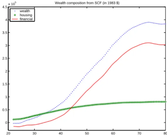
Appendix 8.1 describes the implication of this standard life cycle model in greater detail. 20 30 40 50 60 70 80 0 0.5 1 1.5 2 2.5 3 3.5 4 4.5x 10
5 Wealth composition from SCF (in 1983 $) wealth
housing financial
Figure 8: Age profile of wealth composition
I now show the patterns of wealth accumulation and portfolio composition over the life cycle. Figure 8 plots mean net worth, housing stock, financial assets against the head of the household’s age. Young agents tend to hold little wealth. Early in life households borrow to buy houses, and thus save in the form of housing. As time goes by, agents have built stocks of houses and start to increase their holding of financial assets. The profiles of financial assets and housing assets intersect in their early 40’s. Their wealth holding peaks at age 70. However, we do not observe quick decumulation of wealth later in life. Instead, households continue to hold large amount of wealth.
3
The Model
The economy is a discrete-time overlapping generation world with an infinitely-lived govern-ment. The government taxes labor earnings, and provides pensions to the retirees. There are idiosyncratic income shocks. There are no state contingent markets for the household specific shocks. The only financial instrument is a one-period bond. Housing has a dual role: it pro-vides utility as consumption goods, and it can be used as collateral thus the borrowing limit of each household depends on the value of the house. Trading of houses incurs transaction costs. For simplicity, I assume there is no housing rental market.
3.1 Technology
There is one type of goods produced according to the aggregate production functionF(K;L)
where K is the aggregate capital stock and L is the aggregate labor input. I assume a
standard Cobb-Douglas functional form. The final goods can be either consumed or invested into physical capital or transformed into housing. Physical capital and housing depreciate at
C the aggregate consumption of non-housing, Ih the aggregate investment on housing, Ik
the aggregate investment on physical capital goods,T cthe total transaction costs for trading
housing, respectively. The aggregate resource constraint is:
(1) F(K, L) =KαL1−α=C+Ik+Ih+T c.
Households rent capital and efficient labor units to the representative firm each period
and receive rental income at the interest rate r and wage income at the wage ratew.
3.2 Demographics
During each model period, which is 5 years long, a continuum of people is born. I denote
aget= 1 as 20 years old, aget= 2 as 25 years old, and so on. At age 20 each person enters
into the model and start working and consuming. Since there are no inter-vivos transfers, all agents start their economic life with no financial assets and no houses. At the beginning of period 3, the agent’s children are born, and four periods later (when the agent is 50 years
old) the children are 20 and start working. The agents are retired att= 10 (i.e., when they
are 65 years old) and die for sure by the end of age T = 12 (i.e., before turning 80 years
old). Fromt= 10 (i.e., when they are 65 years old), each person faces a positive probability
of dying given by (1−pt). The probability of dying is exogenous and independent of other
household characteristics. The population grows at rate n. Since the demographic patterns
are stable, agents at age t make up a constant fraction of the population at any point in
time. Figure 9 illustrates the demographics in the model.
3.3 Timing and information
At the beginning of each period, households observe their idiosyncratic earning shocks and possibly receive some inheritance from their parents. Then labor and capital are supplied to firms and production takes place. Next, the households receive factor payments and make their consumption and asset allocation decisions. Housing stocks are not transferred until the end of the period. Thus the addition or subtraction to the stock will not influence the present period service flow. Finally uncertainty about early death is revealed.
The idiosyncratic labor productivity status is private information and the survival status is public information. I assume that children can observe their parent’s productivity when their parent is 50 and the children are 20.
3.4 Consumer’s maximization problem
3.4.1 Preferences
Individuals derive utility from consumption of non-housing goods, c, from the service flow
Generation t-6
(Parents) 50 55 60 65 70 75 80
Generation t
20 25 30 35 40 45 50 55 60 65 70 75 80 procreate death shock
Generation t+6
(Children) 20 25 30 35 40 45 50
Figure 9: Demographics
are assumed to be time separable, with a constant discount factorβ. The momentary utility
function from consumption is of the constant relative-risk aversion class given by
(2) U(c, h) = g(c, h)1−η−1
1−η .
I chooseg(c, h) = (ωcσ+ (1−ω)hσ)1σ,and h is assumed to be equal to the value of housing
stock.
Following De Nardi (2004), the utility from bequest is denoted by
(3) φ(b) =φ1(1 +b/φ2)1−η.
The term φ1 reflects the parent’s concern about leaving bequests to his/her children, while
φ2 measures the extent to which bequests are luxury goods3.
3.4.2 Transaction costs
Due to the heterogeneity of housing and the spatial fixity of housing, both potential buyers and sellers in the housing market are forced to spend considerable amount of time and resource
3Note that this form of ‘impure’ bequest motives implies that an individual cares about the bequests left
to his/her children, but not about consumption of his/her children. If an individual is assumed to care about utility of his/her children, and both parents and kids are maximizing utility as different units, the strategic interaction across generations complicates the analysis.
to acquire information about the value of a specific housing units. As a consequence, there are both implicit and explicit search costs associated with moving (Chinloy (1980)). These include opportunity cost of time associated with market search, brokerage and agent fee, recording fee, legal fee, origination fee. Besides, households have to physically move to a new house, which entail moving costs and psychological costs of breaking neighborhood attachments (Smith, Rosen, Fallis (1988)).
I consider non-convex transaction costs in the housing stock. A household can buy a stock of any size, but once the stock has been bought, it is illiquid. I force the household to pay transaction costs every time the household sells and buys a new house. The specification of the transaction costs is:
(4) τ(h, h0) =
(
0 ifh0 ∈[(1−µ
1)h, (1 +µ2)h]
ρ1h+ρ2h0 otherwise.
This formulation of transaction costs allow households to change their level of housing
consumption by undertaking housing renovation up to a fraction of µ2 the value of house or
by allowing depreciation up to a fraction ofµ1 the value of house as an alternative to moving.
If the households let the housing depreciate by more that a fractionµ1 of the value, or if the
value of the stock increases by more that a fractionµ2 of the value, I assume that the stock
has been sold. In those cases, the household has to pay the transaction costs as a fractionρ1
of its selling value and ρ2 of its buying value.
3.4.3 Borrowing constraints
I assume that only collateralized credit is available and that the borrowing interest rate, mortgage interest rate and deposit interest rate are all equal. This implies that mortgages
and deposits are perfect substitutes. I use at to denote the net asset position. To buy a
house household must satisfy a minimum down payment requirement as a fraction θ of the
value of house. Housings also serves as collateral for loans (through home equity loans or
refinancing) up to a fraction (1−θ). At any given period household’s financial assets must
hence satisfy:
(5) a0 ≥ −(1−θ)h0,
and household’s net worth is thus always non-negative. Notice in this case, a household’s net
worth is bounded below by a fraction θof the value of house4.
3.4.4 Labor productivity
In this economy all agents of the same age face the same exogenous age-efficiency profile²t.
This profile is estimated from the data and recovers the fact that productive ability changes over the life cycle. Workers also face stochastic shocks to their productivity level. These
shocks are represented by a Markov process defined on (Y;B(Y)) and characterized by a
transition functionQy, where Y ⊂R++ and B(Y) is the Borel algebra onY. This Markov
process is the same for all households. This implies that there is no aggregate uncertainty over the aggregate labor endowment although there is uncertainty at the individual level.
The total productivity of a worker of agetis given by the product of the worker’s stochastic
productivity in that period and the worker’s deterministic efficiency index at the same age:
yt²t.
To capture the positive correlation in human capital across generations, I assume that the parent’s productivity shock at age 50 is transmitted to children at age 20 according to a
transition function Qyh, defined on (Y;B(Y)). What the children inherit is only their first
draw; from age 20 on, their productivity yt evolves stochastically according toQy.
For computational reasons, I assume that children cannot observe directly their parent’s assets, but only their parent’s productivity when their parent is 50 and the children are 20,
that is, the period when they leave the house and start working5. Based on this information,
children infer the size of the bequests they are likely to receive.
3.4.5 The household’s recursive problem
In the stationary equilibrium, the household’s state variables are given by (t, a, h, y, yp),the
first 4 variables of which denote the agent’s age, financial assets and housing stock carried
from the previous period and the agent’s productivity, respectively. The last termypdenotes
the value of the agent’s parent’s productivity at age 50 until the agent inherits and zero
thereafter. The law of motion of yp is dictated by the death probability of the parent.
When ypis positive, it is used to compute the probability distribution on bequests that the
household expects from the parent. When the agents have already inherited,yp is set to be
0.
According to the demographic transitions, there are four cases.
(i) From t= 1 to t= 3 (from age 20 to 35), the agent survives with certainty until next
period and does not expect to receive a bequest soon because his or her parent is younger
than 65. For these sub periodsyp0 =yp.
(6) V(t, a, h, y, yp) = max c,a0,h0
n
U(c, h) +βE(V(t+ 1, a0, h0, y0, yp))
o
5For example, allowing children to observe parents productivity at two periods adds one more state variable
and also increases substantially the time needed to iterate over the bequest distributions. Since income in the calibration is very persistent, an observation of one year of income is likely to be not much less informative than two.
subject to (5) and
c+a0+h0+τ(h0, h) = (1−τl)w²+ (1 +r)a+ (1−δh)h,
(7)
c ≥ 0, h0 ≥0.
(8)
At any subperiod, the agent’s resources are derived from asset holdings,a, labor
endow-ment, ²tyhousing stock holding,h. Asset holdings pay a risk-free rater and labor receives a
real wagew. Houses depreciate at rateδh. The evolution ofy is described by the transition
functionQy.Government taxes labor income at the rateτl.
(ii) From t= 4 to t= 6 (from age 35 to 50), the worker survives for sure until the next
period. However, the agent’s parent is at least 65 years old and faces a positive probability of dying at any period; hence, a bequest might be received at the beginning of the next period.
The conditional distribution of bequest a person of statex expects in case of parental death
is denoted by µb(x; :). In equilibrium this distribution must be consistent with the parent’s
behavior. Since the evolution of the state variableypis dictated by the death process of the
parent, yp0 jumps to zero with probability 1−pt+6. LetIyp>0 be the indicator function for
yp >0; it is one ifyp >0 and zero otherwise.
(9) V(t, a, h, y, yp) = max c,ea,h0 n U(c, h) +βE(V(t+ 1, a0, h0, y0, yp0)) o subject to (5), (8), and c+ea+h0+τ(h0, h) = (1−τl)w²+ (1 +r)a+ (1−δh)h, a0 = ea+b0Iyp>0Iyp0=0, (10)
whereea denotes the financial assets at the end of the period before receiving bequest.
(iii) The subperiodst= 7 to t = 9 (from age 50 to 65) is the periods before retirement,
during which no more inheritances are expected because the agent’s parent is already dead
by that time. Thus yp is not in the state space any more. The agent does not face any
survival uncertainty. (11) V(t, a, h, y) = max c,a0,h0 n U(c, h) +βE(V(t+ 1, a0, h0, y0)) o subject to (5), (7) and (8).
(iv) From t= 10 to t = 12 (from age 65 to 80), the agent does not work and does not
inherit any more, but faces a positive probability of dying. Let pt denote the conditional
survival probability at age t. In case of death, the agent derives utility from bequeathing his
incurred6. (12) V(t, a, h) = max c,a0,h0 n U(c, h) +βpt(V(t+ 1, a0, h0)) + (1−pt)φ(b) o subject to (5), (8) and c+a0+h0+τ(h0, h) = (1 +r)a+ (1−δh)h+P, (13) b=a0+h0−τ(h0,0).
Households receive pension income P. For simplicity, I assume the pension level is
inde-pendent of household’s income history7.
4
Calibration
I choose some parameters used in the benchmark model from estimations by other studies. The remaining parameters are chosen so that the model generated data match a given set of targets. Since one period in my model corresponds to 5 years in real life, I adjust parameters accordingly.
The rate of population growth, n, is set to the average population growth from 1950 to
1997 from Economic Report of the President (1998). The pt’s are the vectors of conditional
survival probabilities for people older than 65. I use the mortality probabilities of people born in 1965 provided by Bell, Wade, and Goss (1992).
I construct measures of outputY, capitalK and housingH and their investment
coun-terparts according to my model. I use data from the National Income and Product Accounts and the Fixed Assets Tables both from the Bureau of Economic Analysis for the year 1954-1999. The aggregate ratios for US economy are calibrated to explicitly consider the existence of housing that comprises residential assets. Output is defined as measured GDP minus housing services. Capital is defined as the sum of nonresidential private and government
fixed assets plus the stock of inventories. Investment in capital,I is defined accordingly. The
housing stock is defined as the stock of private residential assets. Investment in housing,Ih,
is constructed accordingly. The term α is the share of income that goes to capital, which
I turns out to be 0.226. This capital share (non residential stock of capital) is much lower
than that in other calibrations, which abstract from housing. The rate r is the interest rate
on capital net of depreciation. I calibrate δk to be 0.0700 and δh to be 0.0294. Given the
calibration for the US production function, this interest rate is endogenous, and turns out to
6I made this simplification since the children already have houses of their own when they inherit.
7A more realistic assumption is that social security benefit is a concave function of the accumulated
contribution. Under this assumption, the accumulated contribution becomes a state variable, which increases the computation time dramatically.
be 4.37%. Appendix 8.5 explains the rationale behind these choices in greater detail.
The deterministic age-profile of the unconditional mean of labor productivity,²t,is taken
from Hansen (1993). Since I impose mandatory retirement at the age of 65, I take²t= 0 for
t >9. The stochastic productivity process is assumed to be an AR(1) process:
lnyt=ρylnyt−1+µt µtvN(0, σ2y).
The persistence ρy and variance σ2y are estimated from Panel Study on Income Dynamics
(PSID) data, aggregated over five years in order to be consistent with the model period (Altonji and Villanueva (2002)). The parent’s productivity shock at age 50 is transmitted to children at age 20 according to the following transition function:
lny1 =ρyhlnyh,7+ν1, ν1 ∼N(0, σyh2 ).
I take ρyh from Zimmerman (1992), and chooseσ2yh to match the Gini coefficient of 0.44 for
earnings.
The down payment ratioθis set to be 0.2, which is commonly used in housing literature.
Recently some households are allowed to purchase houses without much initial wealth. How-ever, Caplin et al. (1997) argue that “it is almost impossible for a household to purchase a home without available liquid assets of at least 10% of the home’s value”. In addition, what is crucial for my model is the assumption that young and poor household can not borrow beyond the liquidation value of their collateral. Thus I choose a higher down payment ratio despite the recent decline of down payment ratio. I see the effect of down payment ratio in Section 6.
Since one of my main interest is to look at how transaction costs affect consumption and saving decisions, one key calibration is the type of transaction costs that I choose. Smith, Rosen and Fallis (1988) estimate the transaction costs of changing houses, including searching, legal costs, cost of readjusting home, and psychological costs from disruption. Their estimation is approximately 8-10 percentage the unit being changed. Martin (2002) finds that the monetary costs of buying a new home, which include agent fee, transfer fee, appraisal and inspection fee, range on average from 7 to 11 percent of purchase price of a home. Gruber and Martin (2003) estimate the reallocation cost of tax and agency costs from CEX and find the median household pays costs of the order of 7 percent to sell their houses and 2.5 percent to purchase. In my simulation, I choose transaction costs from sale to be
ρ1 = 6%,and transaction costs from purchase to be ρ2 = 2%. These values are lower than
the transaction costs reported above therefore they serve as a lower bound of the effect of
transaction costs. I setµ1=µ2 = 0. That is to say, if the value of the housing stock increases
or decreases, I assume that the house has been sold.
The social security income P is chosen to be 40% of the average household after tax
is chosen to balance government budget.
I take risk aversion parameter,η, to be 1.5, from Attanasio et al. (1999) and Gourinchas
and Parker (2002), who estimate it from consumption data. This value is in the commonly
used range (1-5) in the literature. σ governs the elasticity of substitution between housing
and non-housing. Ogaki and Reinhart (1998) use aggregate data and a similar specification,
and obtain an estimated σ = 0.145, not significantly different from zero. I thus choose σ to
be 0 so that the momentary utility function g(c, h) takes the Cobb-Douglas form8. I see the
effect of elasticity of substitution between housing and non-housing in Section 6.
I choose the discount factor, β, to match the capital-output ratio. The parameter ω
determines the share of consumption allocated to the non-housing consumption goods and
is set to match the ratio of non-housing expenditure to housing stock. I use φ1 to match
bequest output ratio of 2.65% in the US simulation (Gale and Scholz (1994))9. φ
2is chosen to
match the ratio of average bequest left by single decedents at the lowest 80th percentile over average household earnings. According to Hurd and Smith (2001), the average bequest left by single decedents at the lowest 80th percentile was $125,000 (Asset and Health Dynamics Among the Oldest Old (AHEAD) data sets, 1993-95).
5
Numerical Results
The benchmark economy allows for housing transaction costs and µ1 = µ2 = 0. That is
to say, if the value of the housing stock increases or decreases, I assume that the house has
been sold. In this case, the household has to pay the transaction costs as a fractionρ1 = 6%
of its selling value and ρ2 = 2% of its buying value. Some parameters are set so that the
model-generated data match a given set of targets (see Section 4). Appendix 8.6 describes the computation algorithm in greater detail.
5.1 Life cycle profiles
Now I show the average life cycle profiles of financial assets, total net worth, non-housing consumption and housing consumption. All figures are normalized by the average household earnings. These averages are obtained by integrating the policy function with respect to the equilibrium measure of agents, holding age fixed. For example, the average housing
consumption by an agent at aget is given by
H=
R
h(t, a, h, y, yp)m∗({t} ×da×dh×dy×dyp) R
m∗({t} ×da×dh×dy×dyp)
Figure 10 compares the average life cycle profiles of annual non-housing consumption and
8In this case I add a positive numberεso that utility function is well defined ath= 0.The termεis small
enough that it does not affect the results. The utility function takes formg(c, h) =cω(h+ε)1−ω 9Since in my model output corresponds to GDP minus housing service, I adjust it accordingly.
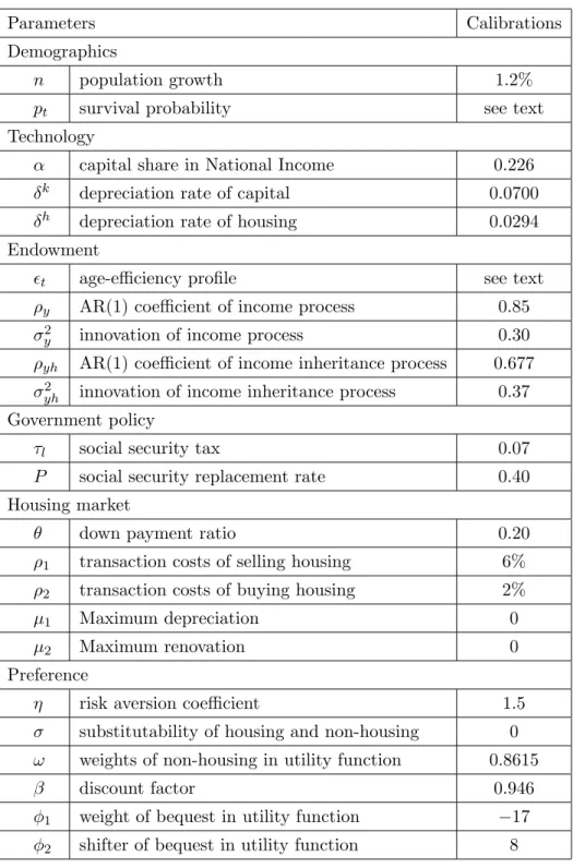
Parameters Calibrations Demographics
n population growth 1.2%
pt survival probability see text
Technology
α capital share in National Income 0.226
δk depreciation rate of capital 0.0700
δh depreciation rate of housing 0.0294
Endowment
²t age-efficiency profile see text
ρy AR(1) coefficient of income process 0.85
σ2
y innovation of income process 0.30
ρyh AR(1) coefficient of income inheritance process 0.677
σ2
yh innovation of income inheritance process 0.37
Government policy
τl social security tax 0.07
P social security replacement rate 0.40
Housing market
θ down payment ratio 0.20
ρ1 transaction costs of selling housing 6%
ρ2 transaction costs of buying housing 2%
µ1 Maximum depreciation 0
µ2 Maximum renovation 0
Preference
η risk aversion coefficient 1.5
σ substitutability of housing and non-housing 0
ω weights of non-housing in utility function 0.8615
β discount factor 0.946
φ1 weight of bequest in utility function −17
φ2 shifter of bequest in utility function 8
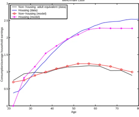
housing consumption in the model with those in the data reported in Figure 3 and Figure 4. I adjust the data so that aggregate non-housing consumption is the same in the data
as in the model10, and aggregate housing stock is the same in the data as in the model.
From Figure 10, we see the hump shape of average non-housing consumption, which peaks at age 50’s. The non-housing consumption at age 50 is 80% more than that of age 20, which is similar to the pattern reported in the data. After the peak, non-housing consumption decreases steadily with age. The non-housing consumption at age 50 is 25% more than that of age 75. Facing an increasing future income profile, young agents would like to borrow to finance their current consumption but they are borrowing constrained. This explains why early in life consumption path increases as income path does. As households age, they start to decrease their non-housing consumption due to the fact that time preference is higher than the interest rate and mortality rates are increasing along the life cycle. Compared with data, the non-housing consumption is lower between age 20-35. This may be due to the abstraction of inter-vivos transfers or housing rental market in the model. Inter-vivos transfer relaxes borrowing constraints, while a housing rental market allows young households to have high non-housing consumption while renting. For detailed discussions of the implications of those two limitations, see Section 7.
20 30 40 50 60 70 80 0 0.5 1 1.5 2 2.5 3 Benchmark Case
Consumption/average household earnings
Age Non−housing: adult equivalent (data) Housing (data)
Non−housing (model) Housing (model)
Figure 10: Life cycle patterns of consumption (benchmark)
The housing consumption profile in the model reproduces the empirically observed in-creasing early in life and slow downsizing later in life. Agents build their housing stock early in life and compromise on non-housing consumption. Agents build up their highest housing stock at the age of 60, 5 years later than the peak of non-housing consumption. The elderly do not decrease their housing stock later in life.
The model also generate the pattern that the ratio of housing to non-housing consumption
10In the model I match the aggregate consumption with this in the NIPA. Compared with NIPA, CEX
underreports consumption by a fraction of 30% (see Attanasio, Battistin and Ichimura (2004) for detailed discussion). Thus I adjust for the difference accordingly.
20 30 40 50 60 70 80 0 0.5 1 1.5 2 2.5 3 3.5 Benchmark Case Housing/non−housing consumption Age data
data (adult equivalent) benchmark model aggregate h/aggregate c
Figure 11: Ratio of housing to non-housing consumption (benchmark)
increases over the life-cycle. Figure 11 compares this ratio in the model and in the data. Early in life, the ratio of housing to non-housing is higher than that in the data. This is because in the model non-housing consumption is lower than that in the data. Later in life, the ratio of housing to housing is lower than that in the data. This is because in the model non-housing consumption is higher than in the data. A parsimonious model without borrowing constraints and transaction costs in trading houses implies a constant ratio of housing to
non-housing consumption, which is equal to HC. If we denote the difference in the ratio between
the data and the parsimonious model without borrowing constraints and transaction costs in trading houses to be 1, the model account for 60% of the difference.
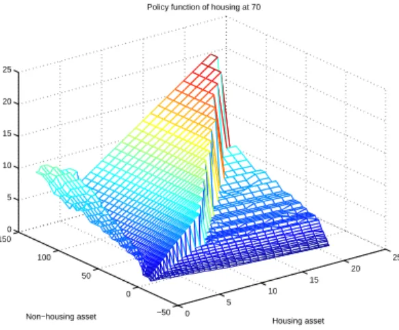
0 5 10 15 20 25 −50 0 50 100 150 0 5 10 15 20 25 Housing asset Policy function of housing at 70
Non−housing asset
Figure 12: Policy function of housing stock next period for a 70-year-old
The introduction of transaction costs forces agents to reduce the frequency of transactions in the housing market. Agents make no change to the stock of the housing unless their non-housing assets and non-housing stocks are too unbalanced. Two retired agents with the same housing stock, age and different holding of non-housing assets may choose the same level
of housing stock next period, as long as the difference of non-housing assets is not large. Given current housing stock, there is a wide range of non-housing assets that households do not adjust for their housing stock. The size of the inactive region is different according to agents age and income and also is affected by parameters such as the size of the transaction costs. Figure 12 shows the policy function of housing next period as a function of current holding of non-housing and housing stock for a 70-year-old agent. Even for relatively small transaction costs, the inactive region is quite large. The inactive region can be defined by
two boundaries, (al(h), ah(h)). If a household with a housing stock ofh holds non-housing
assets more than the upper boundaryah(h),the household will move to a bigger house next
period and hold a smaller fraction of non-housing assets in the wealth portfolio. If instead
he/she holds non-housing assets less than the lower boundaryal(h),the household will move
to a smaller house next period and hold a larger fraction of non-housing assets in the wealth portfolio. Figure 13 shows the boundaries of the inactive region on the plane of current holding of non-housing and housing stock for a 70-year-old agent and a 65-year-old agent, respectively. One reason that the inactive region for a 65-year-old agent is smaller than a 70-year-old agent is because a 65-year-old agent has a longer life expectancy which increases the benefit of changing the housing stock. Since bequest is modeled as luxury goods, the utility function is not homothetic. Thus the policy functions are not necessarily homogeneous and the boundaries are not strict lines.
2 4 6 8 10 12 14 16 18 20 0 50 100 150 200 250 Housing asset Non−housing asset Boundary 65 70
Figure 13: Boundaries of inactive zones
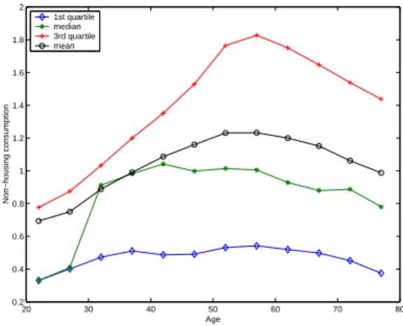
Now we go beyond mean consumption and look at the distribution of consumption in the benchmark economy. Figure 14 plots non-housing consumption at the mean level and at each quartile. We observe that the non-housing consumption is hump-shaped at each quartile. The benchmark economy also generates the skewed distribution of consumption at each age group, as is observed in the data.
Figure 15 plots housing consumption at the mean level and at each quartile. The bench-mark economy generates the increasing of housing stock early in life and the flat portion later
20 30 40 50 60 70 80 0.2 0.4 0.6 0.8 1 1.2 1.4 1.6 1.8 2 Age Non−housing consumption 1st quartile median 3rd quartile mean
Figure 14: Non-housing consumption (quartiles)
in life at each quartile. The benchmark economy also generates the skewed distribution of housing consumption at each age group, as is observed in the data.
20 30 40 50 60 70 80 0 0.5 1 1.5 2 2.5 3 3.5 Age Housing stock 1st quartile median 3rd quartile mean
Figure 15: Housing consumption (quartiles)
The existence of transaction costs affects young agents and old agents differently. Young households face increasing income profiles and would like to purchase large houses but they have to accumulate enough non-housing assets to pay the down payment. As a result, they have to increase their housing stock fairly often. As the households age and their income profile stabilize, households would keep their level of housing stock unchanged, giving that trading of housing stock would incur transaction costs. Old households are less likely to move than young household, since they could only consume the new house for a relatively short period of time. Figure 16 shows the fraction of households moving at the end of each period for each age group. Moving rates by age in the data is taken from Schachter (2001) and are aggregated to five years. We see moving rates decline with age in the model, as in the data. Moving rates in the data is higher than in the model. One reason is that renters are also
20 25 30 35 40 45 50 55 60 65 70 0 10 20 30 40 50 60 70 80 90 100
Moving rates by age (in percent)
Age
Model Data
Figure 16: Moving rates by age
included in calculating the moving rates, and renters tend to move much more frequently than homeowners. The other reason is, households move for reasons other than income shocks and aging that this model abstracts from.
20 30 40 50 60 70 80 −2 0 2 4 6 8 10 12 Benchmark Case
Weath/average household earnings
Housing Non−housing assets Networth
Figure 17: Life cycle patterns of wealth composition
Figure 17 displays the evolution of wealth portfolio over the life cycle. Young agents tend to hold little wealth. They start with zero wealth and they expect to have much higher earnings in the future. Thus to smooth consumption, they do not hold much wealth. Early in life households borrow as much as possible to buy houses, and thus save in the form of housing. As time goes by, agents have built stocks of houses and start to increase their holding of financial assets. The profile of financial assets and housing assets intersect in their early 40’s, as is observed in the data. The wealth holding peaks at age 65, the year before retirement. After retirement, they start to dissave assets to finance consumption. Old agents discount their future consumption at a higher rate since the survival probabilities are declining in age. This implies that the consumption profile is declining later in life and hence
little wealth is needed to finance consumption later in life. Compared with data reported in Figure 8, the wealth profile and assets profile have humps that are more pronounced. Since I abstract from health expenditure uncertainty or other shocks that could motivate precautionary assets holding in old age, old agents do not have precautionary saving motives as they do in the data, therefore they run down their assets more quickly than in the data.
5.2 Wealth distribution
Table 3 reports values for the wealth distribution for my benchmark economy. I present quintile shares, the 90-95%, the 95-99%, the top 1% shares and Gini coefficient for net worth, housing stocks and financial assets. US wealth distribution is calculated using 1998 SCF. In the data wealth is highly unevenly distributed with a Gini coefficient of 0.80. The top 1% of the households hold 34% of the total wealth and the 95-99% of the households hold 24% of the total wealth. Housing is more evenly distributed than net worth with a Gini coefficient of 0.63. The top 1% of the households hold 11% of the total housing wealth and the 95-99% of the households hold 17% of the total housing wealth. Financial asset is more unevenly distributed than net worth with a Gini coefficient of 0.99. The top 1% of the households hold 46% of the total financial wealth and the 95-99% of the households hold 28% of the total
financial wealth11.
The benchmark model matches the distribution of wealth, housing and financial wealth quite well, with the exception of top 1%. It also replicates the empirical finding that inequality in financial assets is much higher than housing. This is because households are allowed to borrow against housing so financial assets can be negative but the housing stock can not be. Also for households that are not borrowing constrained, the return of housing, marginal utility of housing, is decreasing, while the return to financial assets, the interest rate, is constant. Thus housing as the fraction of net worth is decreasing.
5.3 Bequest distribution
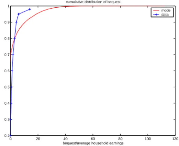
Figure 18 compares the cumulative distribution of estate among the whole economy at any given time implied by the model with the data. The US data on the estate distribution is from Hurd and Smith (2001) who use the AHEAD data exit interview of 771 deceased
between 1993-199512. The size distribution of the bequest is very concentrated both in the
data and in the model: 30% of the deceased AHEAD respondents had an estate of no value13.
11All Gini coefficients are calculated without replacing the negative numbers with zeros. If I replace the
negative numbers with zeros, then the Gini coefficients become slightly smaller
12I use distribution for single decedents. Using the bequest left by singles rather than the one for all
decedents (which turns out to be 1-2 times bigger) is a more sensible choice because typically a surviving spouse inherits a large share of the estate, which will be partly consumed before finally being left to the couple’s children.
1330% households report leaving no bequest in AHEAD but 70% households report receiving no inheritance
Gini 1st 2nd 3rd 4th 5th 90-95 95-99 99-100 Total wealth U.S. data 0.80 -0.28 1.35 5.14 13.00 81.59 11.48 23.72 33.65 Model 0.74 0.13 0.67 4.04 17.35 77.81 19.91 25.12 10.00 Housing US data 0.63 0 1.09 13.66 24.10 61.15 13.87 17.12 11.32 Model 0.48 1.73 8.39 14.71 24.59 50.58 13.02 11.79 3.74 Financial wealth US data 0.99 -6.00 -0.12 1.26 7.23 97.64 11.98 28.20 46.35 Model 0.86 -6.07 -2.68 -0.29 12.32 96.71 24.51 33.70 14.07
Table 3: Wealth distribution
The mean estate was $104,500 but the median was much lower ($62,200). Some respondents leave relatively large estates: 30% are $120,000 or more and 5% are in excess of $300,000. Only 3% of the estates were valued at $600,000 or more. One parameter of the model is chosen so that the two distributions match at one point: the 80th percentile. The estate distribution generated by the model actually matches very well to the AHEAD data until the 80th percentile of the estate distribution. From that point on, the model predicts larger bequests than those observed in the AHEAD data. The discrepancy is partly due to the fact that AHEAD misses some large estates.
0 20 40 60 80 100 120 0.2 0.3 0.4 0.5 0.6 0.7 0.8 0.9 1
cumulative distribution of bequest
bequest/average household earnings
model data
Figure 18: Cumulative distribution of bequest
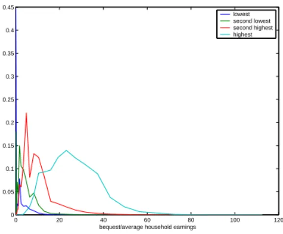
Figure 19 shows the bequest distribution for a 35-year-old person conditional on his/her parent’s observed productivity level. At that age, the probabilities of receiving bequests less than 2 times output per capita are, respectively, 71%, 19%, 1% and 0%, for people with parents in the lowest, second lowest, second highest and highest productivity levels. Even in the presence of bequest motives, most of the parents run down their assets after retirement.
0 20 40 60 80 100 120 0 0.05 0.1 0.15 0.2 0.25 0.3 0.35 0.4 0.45
bequest/average household earnings
lowest second lowest second highest highest
Figure 19: Expected bequest distribution at age 35, conditional on parent’s productivity The fraction of people whose parents live up to the final age of the model economy and who do not receive a positive bequest are, respectively, 99%, 98%, 88% and 23%, for people with parents in the lowest, second lowest, second highest and highest productivity levels.
6
Decomposition
While the benchmark model does a good job in generating the different patterns of housing and non-housing consumption, and the evolution of assets composition, let us now try to understand how each ingredient affects the results. I change one parameter at a time, keeping other parameters as in the benchmark economy. This comparison can shed light on what role each feature of the model plays in generating the consumption and assets accumulation profiles.
First, I change the transaction costs. Then I change the remodeling-maintenance option. I further change parameters that govern the bequest motives. Then I check the effect of down payment ratio. I also change the elasticity of substitution between the housing and the non-housing consumption. Finally I study the effect of the pay-as-you-go social security system.
6.1 Transaction cost
Now I investigate the effects of transaction costs on household consumption and asset hold-ing in this subsection by setthold-ing costs to 0. In Figure 20, we see the hump shape of the average non-housing consumption, which is similar to the one reported in the data and in the benchmark model. Compared with the benchmark case, a model without transaction costs generates a hump-shaped non-housing consumption profile but the decrease of housing stock later in life is too fast.
20 30 40 50 60 70 80 0 0.5 1 1.5 2 2.5 3 Consumption Non−housing (Benchmark) Housing (Benchmark) Non−housing Housing
Figure 20: Life cycle patterns of consumption (no transaction costs: ρ1 =ρ2= 0%)
and without transaction costs. Without transaction costs, the ratio becomes flatter over the life cycle. The ratio is increasing early in life because of the existence of borrowing constraints. Later in life when borrowing constraints are less likely to be binding, a model without trans-action costs implies a flat pattern of the ratio of housing to non-housing consumption. These results show that borrowing constraints are essential in explaining the accumulation of hous-ing assets early in life, while the transaction costs play an important role in explainhous-ing the slow decline of housing consumption later in life.
20 30 40 50 60 70 80 0 0.5 1 1.5 2 2.5 Consumption ratio (h/c) Benchmark noCost aggregate h/c
Figure 21: Ratio of housing to non-housing consumption (no transaction costs: ρ1 =ρ2= 0%)
Figure 22 shows the average life cycle profiles of financial assets and total net worth. The evolution of the wealth portfolio over the life cycle is similar to the one in the benchmark case. The holding of financial assets is lower than the benchmark. This is because without transaction costs, housing assets become more attractive than financial assets. Therefore a household’s portfolio shifts from financial assets to housing assets.
Figure 23 shows the effect of low transaction costs on average non-housing and housing
20 30 40 50 60 70 80 −2 0 2 4 6 8 10 12 Wealth
Non−housing assets (Benchmark) Networth (Benchmark) Non−housing assets Networth
Figure 22: Life cycle patterns of wealth composition (no transaction costs: ρ1=ρ2 = 0%)
20 30 40 50 60 70 80 0 0.5 1 1.5 2 2.5 Consumption Non−housing (Benchmark) Housing (Benchmark) Non−housing Housing
Figure 23: Life cycle patterns of
consump-tion (high transacconsump-tion costs: ρ1 = 3%,
ρ2= 1% ) 20 30 40 50 60 70 80 −2 0 2 4 6 8 10 12 Wealth
Non−housing assets (Benchmark) Networth (Benchmark) Non−housing assets Networth
Figure 24: Life cycle patterns of wealth
composition (high transaction costs: ρ1 =
3%, ρ2 = 1% )
housing consumption is higher than that in the benchmark. This is because when transaction costs are lower, housing assets become more attractive than financial assets. We also see that when the transaction costs are lower, housing consumption declines slightly after age 60. Figure 24 shows that the effect of low transaction costs on net worth profile is small.
Figure 25 shows the effect of high transaction costs on average non-housing and housing
consumption, when I setρ1= 8% andρ2 = 2%. The housing consumption is lower than that
in the benchmark. This is because when transaction costs are higher, housing assets become less attractive than financial assets. Figure 26 shows that the effect of high transaction costs on net worth profile is small.
6.2 Remodeling-maintenance option
Now I give agents the remodeling-maintenance option. I set µ1 =µ2 = 15% (which is equal
20 30 40 50 60 70 80 0 0.5 1 1.5 2 2.5 Consumption Non−housing (Benchmark) Housing (Benchmark) Non−housing Housing
Figure 25: Life cycle patterns of
consump-tion (high transacconsump-tion costs: ρ1 = 8%,
ρ2= 2% ) 20 30 40 50 60 70 80 −2 0 2 4 6 8 10 12 Wealth
Non−housing assets (Benchmark) Networth (Benchmark) Non−housing assets Networth
Figure 26: Life cycle patterns of wealth
composition (high transaction costs: ρ1 =
8%, ρ2 = 2% )
level of housing consumption by allowing depreciation up to 15% the value of the house or by undertaking housing renovation up to a fraction of 15% the value of the house as an alternative to moving. 20 30 40 50 60 70 80 0 0.5 1 1.5 2 2.5 Consumption Non−housing (Benchmark) Housing (Benchmark) Non−housing Housing
Figure 27: Life cycle patterns of con-sumption (remodeling-maintenance
op-tion: µ1 =µ2= 15%) 20 30 40 50 60 70 80 −2 0 2 4 6 8 10 12 Wealth
Non−housing assets (Benchmark) Networth (Benchmark) Non−housing assets Networth
Figure 28: Life cycle patterns of wealth
composition (remodeling-maintenance
option: µ1 =µ2= 15%)
From Figure 27, we see the same hump-shaped non-housing consumption profile. Housing stock is slightly higher than the benchmark model between age 25-35. This shows that most households would rather upsize their housing stock a lot therefore the remodeling-maintenance option has little effect. Only when at the last period, we see elderly households take the advantage of this option and allow the house to depreciate.
Figure 28 shows the average life cycle profiles of financial assets and total net worth. The evolution of the wealth portfolio over the life cycle is almost identical to the one in the benchmark case.
6.3 Bequest motive
Now I present the results from a model without voluntary bequest motives by settingφ1 = 0.
This modification removes a saving motive thus the aggregate capital stock and output are lower than in the benchmark economy. Figure 29 compares the average non-housing and housing consumption in the case of no bequest motives and in the benchmark case. Compared with the benchmark case, the profiles of housing and non-housing consumption have the similar shape, but the consumption of non-housing goods and housing is lower from age 45 and on. The reason is households are now receiving accidental bequest, which is much smaller than in the benchmark economy with bequest motives, therefore they have less resources to support consumption after middle age. The bequest motives are not the key factor explaining the slow downsizing of housing stock later in life for the average household. The intuition here is that the household faces transaction costs to downsize his/her housing stock, but can run down his/her financial assets without any costs. Without bequest motives, he/she chooses to run down his/her net worth completely by the time he/she expects to be dead for sure. Thus it is optimal to do so by running down his/her financial assets, rather than by trading the large house he/she lives in to a smaller one, and thus paying large
transaction costs in the process14.
20 30 40 50 60 70 80 0 0.5 1 1.5 2 2.5 Consumption Non−housing (Benchmark) Housing (Benchmark) Non−housing Housing
Figure 29: Life cycle patterns of
consump-tion (no bequest motives: φ1=0)
20 30 40 50 60 70 80 −2 0 2 4 6 8 10 12 Wealth
Non−housing assets (Benchmark) Networth (Benchmark) Non−housing assets Networth
Figure 30: Life cycle patterns of wealth
composition (no bequest motives: φ1=0)
Figure 30 compares the average life cycle profiles of financial assets and total net worth in the case of no bequest motives and in the benchmark case. Compared with the benchmark case, the profiles of financial assets and total net worth is much lower from age 45. The reason is that accidental bequest received is much smaller than in the benchmark economy. The bequest motives, therefore, play an important role in determining total life time wealth
14In the model, mortgages and deposits are perfect substitutes therefore the net mortgage position is
inde-terminant. The fact that households run down their financial assets does not necessary mean that households are borrowing against their houses using reverse mortgage products. The fraction of households aged 65 and above who hold wealth more than the value of the house are still pretty high, around 70% in the benchmark economy, and 67% in the case without bequest motive.