6SDUVH/HDVWWULPPHGVTXDUHVUHJUHVVLRQ
$QGUHDV$OIRQV&KULVWRSKH&URX[DQG6DUDK*HOSHU
DEPARTMENT OF DECISION SCIENCES AND INFORMATION MANAGEMENT (KBI)
SPARSE LEAST TRIMMED SQUARES REGRESSION
By Andreas Alfons, Christophe Croux and Sarah Gelper
K.U.Leuven, K.U.Leuven and Erasmus University Rotterdam
Sparse model estimation is a topic of high importance in mod-ern data analysis due to the increasing availability of data sets with a large number of variables. Another common problem in applied statistics is the presence of outliers in the data. This paper combines robust regression and sparse model estimation. A robust and sparse estimator is introduced by adding an L1 penalty on the coefficient estimates to the well known least trimmed squares (LTS) estimator. The breakdown point of this sparse LTS estimator is derived, and a fast algorithm for its computation is proposed. Both the simulation study and the real data example show that the LTS has better pre-diction performance than its competitors in the presence of leverage points.
1. Introduction. In applied data analysis, there is an increasing avail-ability of data sets containing a large number of variables. Linear models that include the full set of explanatory variables often have poor prediction performance as they tend towards having large variance. Furthermore, large models are in general difficult to interpret. In many cases, the number of variables is even larger than the number of observations. Traditional meth-ods such as least squares can then no longer be applied due to the rank deficiency of the design matrix.
To improve prediction accuracy and as a remedy to computational prob-lems with high-dimensional data, a penalty term on the regression coeffi-cients can be added to the objective function. This shrinks the coefficoeffi-cients and reduces variance at the price of an increased bias.Tibshirani(1996) in-troduced the least absolute shrinkage and selection operator (lasso), which uses theL1 norm as penalty function. Let y= (y1, . . . , yn)0 be the response andX = (xij)1≤i≤n,1≤j≤pthe matrix of predictor variables, wherendenotes
the number of observations and p the number of variables. In addition, let x1, . . . ,xnbe thep-dimensional observations, i.e. the rows ofX. We assume
a standard regression model
(1.1) yi =x0iβ+εi,
Keywords and phrases: Breakdown Point, Outliers, Penalized regression, Robust re-gression, Trimming
where the regression parameter isβ = (β1, . . . , βp)0, and the error termsεi
have zero expected value. With a penalty parameterλ, the lasso estimate of β is (1.2) βˆlasso = argmin β n X i=1 (yi−x0iβ)2+nλ p X j=1 |βj|.
The lasso is frequently used in practice since theL1 penalty allows to shrink some coefficients to exactly zero, i.e., to produce sparse model estimates that are highly interpretable. In addition, a fast algorithm for computing the lasso is available through the framework of least angle regression (LARS; Efron et al., 2004). Other algorithms are available as well (e.g. Wu and Lange,
2008). Due to the popularity of the lasso, its theoretical properties are well studied in the literature (e.g., Knight and Fu, 2000; Zhao and Yu, 2006;
Zou, Hastie and Tibshirani,2007), and several modifications and have been proposed (e.g.Yuan and Lin,2006;Gertheiss and Tutz,2010;Radchenko and James,2011;Wang et al.,2011). However, the lasso is not robust to outliers. In this paper we formally show that the breakdown point of the lasso is 1/n, i.e. only one single outlier can make the lasso estimate completely unreliable. Therefore robust alternatives are needed.
Outliers are observations that deviate from the model assumptions, and are a common problem in the practice of data analysis. Robust alternatives to the least squares regression estimator are well known and studied, see
Maronna, Martin and Yohai (2006) for an overview. In this paper focus is on the the least trimmed squares (LTS) estimator introduced byRousseeuw
(1984). This estimator has a simple definition, is quite fast to compute, and is probably the most popular robust regression estimator. Denote the vector of squared residuals by r2(β) = (r12, . . . , r2n)0 with ri2 = (yi −x0iβ)2, i= 1, . . . , n. Then the LTS estimator is defined as
(1.3) βˆLTS = argmin β h X i=1 (r2(β))i:n,
where (r2(β))1:n ≤. . . ≤(r2(β))n:n are the order statistics of the squared
residuals and h ≤ n. Thus LTS regression corresponds to finding the sub-set of h observations whose least squares fit produces the smallest sum of squared residuals. The subset size h can be seen as an initial guess of the amount of good observations in the data. While the LTS is highly robust, it clearly does not produce sparse model estimates. Furthermore, ifh < pthe LTS estimator cannot be computed. A sparse and regularized version of the
LTS is obtained by adding anL1 penalty with penalty parameterλto (1.3), leading to thesparse LTS estimator
(1.4) βˆsparseLTS= argmin β h X i=1 (r2(β))i:n+hλ p X j=1 |βj|.
We prove in this paper that sparse LTS has a high breakdown point. It is resistant to multiple regression outliers, including leverage points. Besides being highly robust, and similar to the lasso estimate, the sparse LTS (i) im-proves the prediction performance through variance reduction if the sample size is small relative to the dimension (ii) ensures higher interpretability due to simultaneous model selection, and (iii) avoids computational problems of traditional robust regression methods in the case of high-dimensional data. The sparse LTS (1.4) can also be interpreted as as a trimmed version of the lasso, since the limit case h = n yields the lasso again. Other robust versions of the lasso have been considered in the literature. Most of them are penalized M-estimators, as invan de Geer (2008) andLi, Peng and Zhu
(2011).Rosset and Zhu (2004) proposed to use a Huber-type loss function, which requires knowledge of the residual scale. A least absolute deviations (LAD) type of estimator is proposed byWang, Li and Jiang (2007),
(1.5) βˆLAD-lasso= argmin β n X i=1 |yi−x0iβ|+nλ p X j=1 |βj|.
However, none of these methods is robust with respect to leverage points, i.e. outliers in predictor space, and can only handle outliers in the response variable. The main competitor of the sparse LTS is robust least angle regres-sion, called RLARS, and proposed in Khan, Van Aelst and Zamar (2007). They develop a robust version of the LARS algorithm, essentially replac-ing correlations by a robust type of correlation, to sequence and select the most important predictor variables. Then a non-sparse robust regression es-timator is applied to the selected predictor variables. RLARS, as will be confirmed by our simulation study, is robust with respect to leverage points. A main drawback of the RLARS algorithm ofKhan, Van Aelst and Zamar
(2007) is the lack of an natural definition, since it is not optimizing a clearly defined objective function.
The rest of the paper is organized as follows. In Section2, the breakdown point of the sparse LTS estimator is obtained. A detailed description of the proposed algorithm to compute the sparse LTS regression estimator is provided in Section 3. Section 4 introduces a reweighted version of the estimator in order to increase statistical efficiency. The choice of the penalty
parameter λ is discussed in Section 5. Simulation studies are performed in Section 6. In addition, Section 7 contains a real data example. Finally, Section8 concludes.
2. Breakdown point. The most popular measure for the robustness of an estimator is the replacement finite-sample breakdown point (FBP) of an estimator (e.g Maronna, Martin and Yohai, 2006). Let Z = (X,y) denote the sample. For a regression estimator ˆβ, the breakdown point is defined as (2.1) ε∗( ˆβ;Z) = min ( m n : supZ˜ kβˆ(Z0)k2 =∞ ) ,
whereZ˜ are corrupted data obtained fromZ by replacingmof the original
ndata points by arbitrary values. We obtained the following result for the breakdown point of the sparse LTS estimator. The proof is in the appendix.
Theorem1. The breakdown point of the sparse LTS estimatorβˆsparseLTS
with subset size h≤nis given by
ε∗( ˆβsparseLTS;Z) =n−h+ 1
n .
Applying Theorem1to the lasso (corresponding toh=n) yields a finite-sample breakdown point of
ε∗( ˆβlasso;Z) = 1
n.
Hence only one outlier can already let the lasso tend to infinity, despite the fact that large values of the regression estimate are penalized in the objective function of the lasso. The non-robustness of the Lasso comes from the use of the squared residuals in the objective function (1.2). Using other convex loss functions, as done in the LAD-lasso or penalized M-estimators, does not solve the problem and also results in a breakdown point of 1/n.
The smaller the value of h, the higher the breakdown point. By taking
h small enough, it is even possible to have a breakdown point larger than 50%. However, we do not envisage to have such large breakdown points. Instead, we suggest to take a value of hequal to a fraction α of the sample size, with α = 0.75, such that the final estimate is based on a sufficiently large number of observations. This guarantees a sufficiently high efficiency, as will be shown in the simulations in Section 6. The resulting breakdown point is then about 1−α = 25%. Notice that the breakdown point does not depend on the dimensionp. Even if the number of predictor variables is
larger than the sample size, a high breakdown point is guaranteed. For the non-sparse LTS, the breakdown point does depend onp, seeRousseeuw and Leroy(2003).
3. Algorithm. We first present an equivalent formulation of the sparse LTS estimator (1.4). For a fixed penalty parameter λ, define the objective function (3.1) Q(H,β) =X i∈H (yi−x0iβ)2+hλ p X j=1 |βj|,
which is the L1 penalized residual sum of squares based on a subsample H⊆ {1, . . . , n} with|H|=h. With
(3.2) βˆH = argmin
β
Q(H,β),
the sparse LTS estimator is given by ˆβHopt, where
Hopt= argmin
H⊆{1,...,n}:|H|=h
Q(H,βˆH).
Hence the sparse LTS corresponds to finding the subset ofh≤nobservations whose lasso fit produces the smallest penalized residual sum of squares. To find this optimal subset, we use an analogue of the FAST-LTS algorithm developed byRousseeuw and Van Driessen (2006).
The algorithm is based onconcentration steps or C-steps. The C-step at iteration k consists of computing the lasso solution based on the current subset Hk, with |Hk| = h, and constructing the next subset Hk+1 from the observations corresponding to the h smallest squared residuals. LetHk
denote a certain subsample derived at iterationkand let ˆβH
k be the
coeffi-cients of the corresponding lasso fit. After computing the squared residuals r2k = (r2k,1, . . . , rk,n2 )0 with r2k,i = (yi −x0iβˆHk)
2, the subsample H
k+1 for
it-erationk+ 1 is defined as the set of indices corresponding to the hsmallest squared residuals. In mathematical terms, this can be written as
Hk+1 =
i∈ {1, . . . , n}:rk,i2 ∈ {(r2k)j:n:j= 1, . . . , h} ,
where (r2k)1:n ≤ . . . ≤ (r2k)n:n denote the order statistics of the squared
residuals. Let ˆβH
k+1 denote coefficients of the lasso fit based onHk+1. Then (3.3) Q(Hk+1,βˆHk+1)≤Q(Hk+1,βˆHk)≤Q(Hk,βˆHk),
where the first inequality follows from the definition of ˆβHk+1, and the sec-ond inequality from the definition ofHk. From (3.3) it follows that a C-step
results in a decrease of the sparse LTS objective function, and that a se-quence of C-steps yields convergence to a local minimum in a finite number of steps.
In order to increase the probability to end up in the global minimum, a sufficiently large number of starting initial subsamples H0 should be used. An initial subsetH0 is constructed as follows. Draw three observations from
the data at random, say xi1, xi2 and xi3. The lasso fit for this elemental subsetof size 3 is then
(3.4) βˆ{i1,i2,i3} = argmin β
Q({i1, i2, i3},β),
and the initial subsetH0 is then given by the indices of the h observations
with the smallest squared residuals with respect to the fit in (3.4). The non-sparse FAST-LTS algorithm uses elemental subsets of sizep, since any OLS regression requires at least as many observations as the dimension p. This would make the algorithm unapplicable if n < p. Fortunately the lasso is already properly defined for samples of size 3, even for large values of p. Moreover, from a robustness point of view, using only three observations is optimal, as it ensures the highest probability of not including outliers in the elemental set.
In this paper, we used m = 500 initial subsets. Following the strategy advised in Rousseeuw and Van Driessen (2006), we perform only two C-steps for allm subsets, and retain them1= 10 subsamples with the lowest values of the objective function. For the reduced number of subsets m1, further C-steps are performed until convergence.
Estimation of an intercept: the regression model in (1.1) does not contain an intercept. It is indeed common to assume that the dependent variable is mean centered and the predictor variables are standardized before applying the lasso. Therefore, when computing the lasso (3.2) on a subsample, one first standardizes the variables using the means and standard deviations computed from the subsample. It is important that the standardization is not done using the mean and standard deviation computed over the full sam-ple, as these will not be robust. When the lasso fit is computed using the R package lars (Hastie and Efron, 2011), the standardization - and retrans-formation of the estimates - is automatically taken care of. We also verified that the centering and standardizations have no impact on the breakdown point of the sparse LTS estimator.
4. Reweighted sparse LTS estimator. Letαdenote the proportion of observations in a subsample, i.e., h = b(n+ 1)αc. Then (1−α) may be interpreted as an initial guess of the proportion of outliers in the data. This initial guess is typically rather conservative to ensure that outliers do not impact the results, and may therefore result in a loss of efficiency. To increase efficiency, a reweighting step that downweights outliers detected by the sparse LTS estimator can be performed.
Under the normal error model, observations with scaled residuals larger than a certain quantile of the standard normal distribution may be declared as outliers. The residual scale estimate associated to the raw sparse LTS estimator is given by (4.1) σrawˆ =kα v u u t1 h h X i=1 (r2)i:n,
withri =yi−x0iβˆSparseLTS, and
(4.2) kα= 1 α Z Φ−1((α+1)/2) −Φ−1((α+1)/2) u2dΦ !−1/2 ,
a factor to ensure that ˆσrawis a consistent estimate of the standard deviation
at the normal model. This allows to compute weights (4.3) wi =
1 if|ri/ˆσraw| ≤Φ−1(1−δ),
0 if|ri/ˆσraw|>Φ−1(1−δ),
i= 1, . . . , n.
In this paper, δ = 0.0125 is used such that 2.5% of the observations are expected to be flagged as outliers in the normal model, which is a typical choice.
Thereweighted sparse LTS estimator is given by the weighted lasso fit (4.4) βˆreweighted= argmin β n X i=1 wi(yi−x0iβ)2+λnw p X j=1 |βj|, with nw = Pn
i=1wi the sum of weights. With the choice of weights given
in (4.3), the reweighted sparse LTS is then nothing else but the lasso fit based on the observations not flagged as outliers. Of course, other weighting schemes could be considered. The residual scale estimate of the reweighted sparse LTS estimator is given by
(4.5) ˆσreweighted =kαw v u u t 1 nw n X i=1 wi(yi−x0iβ)2,
5. Choice of the penalty parameter. In practical data analysis, a suitable value of the penalty parameter λ is not known in advance. We propose to select λ by optimizing the Bayes Information Criterion (BIC), or the estimated prediction performance via cross-validation. The BIC of a given model estimated with shrinkage parameter λis given by
(5.1) BIC(λ) = log(ˆσ) +df(λ)log(n)
n ,
where ˆσ denotes the corresponding residual scale estimate, (4.1) or (4.5), and df(λ) are the degrees of freedom of the model. The degrees of freedom are given by the number of non-zero estimated parameters in ˆβ (see Zou, Hastie and Tibshirani,2007).
As an alternative to the BIC, cross-validation can be used. To prevent that outliers affect the choice of λ, a robust prediction loss function should be used. A natural choice is the root trimmed mean squared prediction error (RTMSPE) with the same trimming proportion as for computing the sparse LTS. In the example in Section7, the data are split randomly in five blocks of approximately equal size. Each block is left out once to fit the model, and the left-out block is used as test data. In this manner, and for a given value ofλ, a prediction is obtained for each observation in the sample. Denote the vector of squared prediction errorse2 = (e21, . . . , e2n)0. Then
(5.2) RTMSPE(λ) = v u u t 1 h h X i=1 (e2) i:n.
To reduce variability, the RTMSE is averaged over 500 different random splits of the data.
The selected λ then minimizes BIC(λ) or RTMSPE(λ) over a grid of values in the interval [0, λ0]. We take a grid with steps of size 0.025 λ0,
where λ0 is an estimate of the shrinkage parameter that would shrink all
parameters to zero, as inEfron et al.(2004).
6. Simulation study. This section presents a simulation study for comparing the performance of various sparse estimators. The sparse LTS estimator is evaluated for the subset size h =b(n+ 1)0.75c. Both the raw and the reweighted version, see Section4, are considered. We prefer to take a relatively large trimming proportion to guarantee a breakdown point of 25%. Adding the reweighting step will then increase the statistical efficiency of the sparse LTS. We make a comparison with the lasso, the LAD-lasso, and
robust least angle regression (RLARS), discussed in the introduction. We se-lected the LAD-lasso estimator as a representative of the class of penalized M-estimators, since it does not need an initial residual scale estimator.
For every generated sample, an optimal value of the shrinkage parameter
λis selected. The penalty parameters for sparse LTS and the lasso are chosen using the BIC, as described in Section 5. For the LAD-lasso, we estimate the shrinkage parameter in the same way as inWang, Li and Jiang (2007). However, ifp > n we cannot use their approach and we use the BIC as in (5.1), with the mean absolute value of residuals (multiplied by a consistency factor) as scale estimate. For RLARS, we add the sequenced variables to the model in a stepwise fashion, and fit robust MM-regressions (Yohai,1987), as advocated inKhan, Van Aelst and Zamar (2007). The optimal model when using RLARS is then again selected via BIC, now using the robust scale estimate resulting from the MM-regression.
The simulations are performed in R (R Development Core Team, 2011) with packagesimFrame(Alfons, Templ and Filzmoser,2010;Alfons,2011), which is a general framework for simulation studies in statistics. Further-more, the package quantreg (Koenker, 2011) is used for LAD and LAD-lasso, andlars(Hastie and Efron,2011) for the lasso. For RLARS, the vari-ables are sequenced using the code by Khan, Van Aelst and Zamar (2007), which is available fromhttp://users.ugent.be/~svaelst/software/RLARS.
html, while the MM-estimators are computed with package robustbase (Rousseeuw et al.,2011)
6.1. Sampling Schemes. The first configuration is similar as inWang, Li and Jiang (2007). The covariates X = (x1, . . . ,xp) are generated from a p-dimensional standard normal distribution. We take p = 20 and n = 50, so the sample size is moderate compared to the dimension. The coefficient vector β = (βj)1≤j≤p is given by β1 = 0.5, β2 = 1, β3 = 1.5, β4 = 2, and βj = 0 for 5≤j≤p. The response variableyis generated according to the regression model (1.1), where the error terms follow a normal distribution withσ= 0.5 for a strong signal-to-noise ratio.
The second configuration is a latent factor model taken fromKhan, Van Aelst and Zamar (2007). From k = 6 latent independent standard normal vari-ables l1, . . . ,lk and an independent standard normal error variable e, the
response variabley is constructed as
y:=l1+. . .+lk+σe,
whereσ is chosen so that the signal-to-noise ratio is 3, i.e.σ =√k/3.With independent standard normal variablese1, . . . ,ep, a set ofp= 50 candidate
predictors is then constructed as xj := lj +τej, j= 1, . . . , k, xk+1 := l1+δek+1, xk+2 := l1+δek+2, .. . x3k−1 := lk+δe3k−1, x3k := lk+δe3k, xj := ej, j= 3k+ 1, . . . , p,
whereτ = 0.3 andδ = 5 so thatx1, . . . ,xkare low-noise perturbations of the
latent variables,xk+1, . . . ,x3k are noise covariates that are correlated with
the latent variables, andx3k+1, . . . ,xpare independent noise covariates. The
number of observations is set ton= 150.
The third configuration covers the case of high-dimensional data. We generate n = 100 observations from a p-dimensional normal distribution
N(0,Σ), withp= 1000. The covariance matrixΣ= (Σij)1≤i,j≤p is given by
Σij = 0.5|i−j|, creating correlated predictor variables. The coefficient vector
β = (βj)1≤j≤p with β1 = β7 = 1.5, β2 = 0.5, β4 = β11 = 1, and βj = 0
forj ∈ {1, . . . , p}\{1,2,4,7,11}, and the response variable is generated ac-cording to the regression model (1.1), where the error terms follow a normal distribution withσ = 0.5.
For each of the three simulation settings, we apply contamination schemes taken from Khan, Van Aelst and Zamar (2007). To be more precise, we consider
1. No contamination
2. Vertical outliers: 10% of the errors terms in the regression model follow a normalN(20, σ), instead of aN(0, σ).
3. Leverage points: Same as in 2., but the 10% contaminated observations contain high-leverage values, by drawing the predictor variables from independentN(50,1) distributions.
This results in a total of 9 different simulations schemes, which we think to be representative for the many different simulation designs we tried out. The first scheme hasnsmall, but still larger thanp, the second scheme follows a factor model, the third setting hasplarge. The choices for the contamination schemes are standard, inducing both vertical outliers and leverage points in the samples.
6.2. Performance measures. Since one of the aims of sparse model es-timation is to improve prediction performance, the different estimators are evaluated by the root mean squared prediction error (RMSPE). For this purpose, n additional observations from the respective sampling schemes (without outliers) are generated as test data, and this in each simulation run. Then the RMSPE is given by
RMSPE( ˆβ) = v u u t 1 n n X i=1 (˜yi−x˜0iβˆ)2,
where ˜yi and ˜xi, i= 1, . . . , n, denote the observations of the response and
predictor variables in the test data, respectively. The RMSPE of the or-acle estimator, which uses the true coefficient values β, is computed as a benchmark for the evaluated methods. We report average RMSPE over all simulation runs.
Concerning sparsity, the estimated models are evaluated by thefalse pos-itive rate (FPR) and the false negative rate (FNR). A false positive is a coefficient that is zero in the true model, but is estimated as non-zero. Anal-ogously, a false negative is a coefficient that is non-zero in the true model, but is estimated as zero. In mathematical terms, the FPR and FNR are defined as FPR( ˆβ) =|{j ∈ {1, . . . , p}: ˆβj 6= 0∧βj = 0}| |{j ∈ {1, . . . , p}:βj = 0}| , FNR( ˆβ) =|{j ∈ {1, . . . , p}: ˆβj = 0∧βj 6= 0}| |{j ∈ {1, . . . , p}:βj 6= 0}| .
Both FPR and FNR should be as small as possible for a sparse estimator, and are averaged over all simulation runs.
6.3. Simulation results. In this subsection, the simulation results for the different data configurations are presented and discussed.
6.3.1. Results for the first sampling scheme. Table 1 shows the simu-lation results for a configuration with uncorrelated predictors, n= 50 and
p= 20, similar as inWang, Li and Jiang(2007). In the case without contam-ination, the LAD-lasso performs best concerning both prediction accuracy and sparsity, as it has the lowest RMSPE and almost perfect FPR and FNR. RLARS and the Lasso also show excellent performance, followed closely by sparse LTS. The reweighting step clearly improves the estimates, which is reflected in the lower values for RMSPE, and it also improves FPR and
Table 1
Results for the first simulation scheme, wheren= 50andp= 20. Root mean squared error of prediction (RMSPE), the false positive rate (FPR) and the false negative rate
(FNR), averaged over 500 simulation runs, are reported for every method.
No contamination Vertical outliers Leverage points
Method RMSPE FPR FNR RMSPE FPR FNR RMSPE FPR FNR Lasso 0.58 0.13 0.00 1.58 0.44 0.12 2.65 0.00 0.69 LAD-lasso 0.55 0.01 0.00 0.58 0.02 0.01 1.79 0.41 0.26 RLARS 0.56 0.18 0.00 0.61 0.22 0.06 0.72 0.52 0.11 Raw sparse LTS 0.71 0.19 0.01 0.67 0.22 0.00 0.65 0.26 0.00 Sparse LTS 0.66 0.16 0.00 0.63 0.20 0.00 0.63 0.23 0.00 Oracle 0.50 0.50 0.50
FNR. It is worth noting that in general the sparse estimators other than LAD-lasso show a tendency towards more false positives.
When vertical outliers are introduced, the results do not change that much. Only the non-robust lasso suffers from a strong influence of these outliers. LAD-lasso is still the best due to better sparsity behavior, but sparse LTS and RLARS are very close with respect to prediction perfor-mance. RLARS leads to a slightly larger FPR than reweighted Sparse LTS, though, and even false negatives occur in some cases. At this point, it should be noted that false negatives in general have a stronger effect on the RMSPE than false positives. A false negative means that important information is not used for prediction, whereas a false positive merely adds a bit of variance to the predicted values. Reweighting still results in a gain in efficiency for sparse LTS.
In the scenario with leverage points in addition to the vertical outliers, sparse LTS exhibits its strengths and clearly performs best. The lowest val-ues for RMSPE are obtained for sparse LTS. In addition, there are no false negatives. The LAD-lasso is highly influenced by the leverage points, which is reflected in the large RMSPE. Also note the considerable amount of false positives and false negatives for the LAD-lasso in presence of leverage points. Surprisingly, also RLARS leads to a significant amount of false positives and some false negatives, but its prediction performance is still competitive. Closer inspection of the RLARS sequences revealed that significant variables frequently appear rather late in the sequence, which explains this behavior. In any case, the influence of the outliers is the strongest on the lasso. Due to the high FNR, the lasso suffers from the largest RMSPE among the
in-Table 2
Results for the second simulation scheme, withn= 150 andp= 50, as inKhan,
Van Aelst and Zamar(2007). Root mean squared error of prediction (RMSPE), the false
positive rate (FPR) and the false negative rate (FNR), averaged over 500 simulation runs, are reported for every method.
No contamination Vertical outliers Leverage points
Method RMSPE FPR FNR RMSPE FPR FNR RMSPE FPR FNR Lasso 1.17 0.09 0.00 2.47 0.54 0.08 2.21 0.00 0.16 LAD-lasso 1.13 0.04 0.00 1.15 0.07 0.00 1.27 0.18 0.00 RLARS 1.14 0.07 0.00 1.12 0.03 0.00 1.23 0.09 0.00 Raw sparse LTS 1.28 0.34 0.00 1.26 0.32 0.00 1.25 0.26 0.00 Sparse LTS 1.23 0.20 0.00 1.22 0.25 0.00 1.21 0.18 0.00 Oracle 0.81 0.81 0.81 vestigated methods.
6.3.2. Results for the second sampling scheme. The simulation results for the second data configuration are displayed in Table2. Keep in mind that this configuration is exactly the same as in Khan, Van Aelst and Zamar
(2007), and that the contamination settings are a subset of the ones applied in their paper as well. In the scenario without contamination, the results are very similar to the previous example. LAD-lasso, RLARS and lasso show excellent performance. The prediction performance of sparse LTS is good, but is has a larger FPR than the other three sparse methods. Also in the case of vertical outliers, the results are similar to before. The non-robust lasso is influenced by the outliers, whereas RLARS, LAD-lasso and sparse LTS keep their excellent behavior. Sparse LTS still has a considerable tendency towards false positives, but the reweighting step is a significant improvement over the raw estimator.
Nevertheless, the effect of the leverage points is quite different for this configuration. Sparse LTS still performs best, but RLARS and LAD-lasso are much less influenced than in the previous configuration. Even though their RMSPE and FPR slightly increase, there are no false negatives in this case. This suggests that the leverage points do not have the same bad leverage effect they had in the previous example.
6.3.3. Results for the third sampling scheme. Table3 contains the sim-ulation results for the high-dimensional data configuration. In the scenario without contamination, RLARS and the lasso perform best with very low
Table 3
Results for the third simulation scheme, withn= 100andp= 1000. Root mean squared error of prediction (RMSPE), the false positive rate (FPR) and the false negative rate
(FNR), averaged over 500 simulation runs, are reported for every method.
No contamination Vertical outliers Leverage points
Method RMSPE FPR FNR RMSPE FPR FNR RMSPE FPR FNR Lasso 0.62 0.00 0.00 2.54 0.08 0.16 2.55 0.00 0.72 LAD-lasso 0.66 0.08 0.00 0.81 0.00 0.01 1.17 0.08 0.00 RLARS 0.60 0.01 0.00 0.71 0.00 0.09 0.91 0.02 0.09 Raw sparse LTS 0.79 0.02 0.00 0.74 0.02 0.00 0.72 0.02 0.00 Sparse LTS 0.74 0.01 0.00 0.70 0.01 0.00 0.70 0.02 0.00 Oracle 0.50 0.50 0.50
RMSPE and almost perfect FPR and FNR. When vertical outliers are added, RLARS still has excellent prediction performance despite some false negatives. We see that the reweighted sparse LTS performs best here. In addition, the prediction performance of the non-robust lasso already suffers greatly from the vertical outliers. In the scenario with additional leverage points, sparse LTS remains stable and is still the best. For RLARS, sparsity behavior according to FPR and FNR does not change significantly either, but there is a small increase in the RMSPE. On the other hand, LAD-lasso already has a considerably larger RMSPE than sparse LTS, and again a higher FPR than the other methods. Furthermore, the lasso is still highly influenced by the outliers, which is reflected in a very high FNR and poor prediction performance.
6.3.4. Summary of the simulation results. Sparse LTS shows the best overall performance in this simulation study, if the reweighted version is taken. Concerning the other investigated methods, RLARS also performs very well, but suffers sometimes from an increased percentage of false neg-atives under contamination. It is also confirmed that the lasso is not robust to outliers. The LAD-lasso still sustains vertical outliers, but is not robust against bad leverage points.
7. Example: Boston housing data. The Boston housing data set, originating with Harrison and Rubinfeld (1978), has been extensively ana-lyzed in the robust statistics literature. We use the corrected version of the data set byPace and Gilley(1997), which is available from StatLib (http:// lib.stat.cmu.edu/datasets/boston_corrected.txt). The data set
con-Table 4
Variables of the Boston housing data.
Name Description
CM EDV Corrected median values of owner-occupied housing
CRIM Crime rate
ZN Proportion of area zoned with large lots
IN DU S Proportion of nonretail business area
CHAS Dummy variable for location contiguous to the Charles River
N OX Levels of nitric oxides
RM Average number of rooms per dwelling
AGE Proportion of structures built prior to 1940
DIS Weighted distances to employment centers
RAD Index of accessibility to radial highways
T AX Full-value property tax rate
P T RAT IO Pupil/teacher ratio
B Proportion of black population
LST AT Proportion of lower status population
LON Geographical longitude
LAT Geographical lattitude
tains various characteristics of houses, demographics, air pollution, and geo-graphical details on 506 census tracts in or nearby Boston. The objective is to relate the median house price to the other characteristics. Table4gives an overview of the variables included in the data. Inspired byPace and Gilley
(1997), we fit the following model with 18 candidate predictors: log(CM EDV) =β0+β1CRIM +β2ZN +β3IN DU S+β4CHAS
+β5N OX2+β6RM2+β7AGE+β8log(DIS) +β9log(RAD) +β10T AX+β11P T RAT IO+β12B
+β13log(LST AT) +β14LON+β15LAT +β16LON2
+β17LAT2+β18(LON·LAT).
The following methods are applied for comparison: raw and reweighted sparse LTS with 25% of trimming, lasso, LAD-lasso, and RLARS. The op-timal value or the shrinkage parameter is selected using cross-validation, as discussed in Section5. The sparse LTS estimator detects a considerable num-ber of observations as outliers, about 10% of the data. Interestingly, the the raw and the reweighted estimator both select the same model, consisting of the 9 predictors with indices (1, 4, 6, 10, 11, 12, 13, 14, 18). This means that the estimated coefficients corresponding to the other indices are equal to zero. Hence the high breakdown sparse LTS method selects the same model
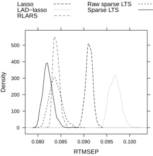
RTMSEP Density 0 100 200 300 400 500 0.080 0.085 0.090 0.095 0.100 Lasso LAD−lasso RLARS Raw sparse LTS Sparse LTS
Fig 1. Density curves of the root trimmed mean squared prediction error (RTMSPE) for the Boston housing data, computed from 500 times repeated fivefold cross-validation.
as the lasso based on the sample with the outliers discarded. Furthermore, LAD-lasso leads to the smallest model under consideration with 6 selected predictors, RLARS selects 8 variables, and the lasso 10.
The prediction performance is estimated via 500 times repeated fivefold CV. Each time, the root trimmed mean squared prediction error (RTMSPE) is computed using 5-fold cross validation, as in (5.2). Figure 1 shows the density curves based on these 500 values of the RTMSPE. Clearly, LAD-lasso exhibits a much higher average RTMSPE, and performs even worse than the lasso. The bad performance of the LAD-lasso is explained by the fact that most of the outliers are bad leverage points, as we verified. Out of the robust methods, the reweighted sparse LTS performs on average better than RLARS or the raw sparse LTS. The gain in efficiency from the reweighting step is clearly visible, as both mean and variance for reweighted sparse LTS are smaller than for the raw version. This example illustrates that sparse LTS gives excellent results in a practical situation with data containing outliers. 8. Conclusions and discussion. Least trimmed squares (LTS) is a ro-bust regression method frequently used in practice. Nevertheless, it does not allow for sparse model estimates and cannot be applied to high-dimensional data ifp > n. This paper introduced the sparse LTS estimator, which
over-comes these two issues simultaneously by adding anL1 penalty to the LTS objective function. Simulation results and a real data example illustrated the excellent peformance of sparse LTS and showed that it performs as well or better than robust variable selection methods such as RLARS. In addition, an advantage of sparse LTS over algorithmic procedures such as RLARS is that the objective function allows for theoretical investigation of its statis-tical properties. As such, we could derive the breakdown point of the sparse LTS estimator. However, it should be noted that efficiency is an issue with sparse LTS. A reweighting step thereby lead to a substantial improvement in efficiency, as shown in the simulation study.
In the paper, anL1penalization was imposed on the regression parameter,
as for the lasso. Other choices for the penalty are possible. For example, an
L2penalty leads to ridge regression. A robust version of ridge regression was recently proposed by Maronna (2011), using L2 penalized MM-estimators.
Even though the resulting estimates are not sparse, prediction accuracy is improved by shrinking the coefficients, and the computational issues with high-dimensional robust estimators are overcome due to the regularization. Another possible choice for the penalty function is the smoothly clipped absolute deviation penalty (SCAD) proposed byFan and Li (2001). It sat-isfies the mathematical conditions for sparsity but results in a more difficult optimization problem than the lasso. Still, a robust version of SCAD can be obtained by optimizing the associated objective function over trimmed samples, instead of over the full sample.
There are several other open questions that we leave for future research. For instance, we did not provide any asymptotics for sparse LTS, as was for example done for penalized M-estimators inGermain and Rouff (2009). Potentially, sparse LTS could be used an an initial estimator for computing penalized M-estimators. Furthermore, for more precise detection of outliers it might be necessary to provide additional finite sample correction correc-tion factors to the scale estimates in (4.1), as was done byPison, Van Aelst and Willems (2002) in the non-sparse case. A very different approach for simultaneous outlier identification and variable selection in linear regression is taken by Menjoge and Welsch (2010). All in all, the results presented in this paper suggest that sparse LTS is a valuable addition to the statistics researcher’s toolbox. The sparse LTS estimator has an intuitively appealing definition, and is related to the popular least trimmed squares estimator of robust regression. It performs model selection, outlier detection, and robust estimation simultaneously, and is applicable if the dimension is larger than the sample size.
PROOF OF BREAKDOWN POINT
Proof of Theorem 1. In this proof, theL1 norm of a vector β is
de-noted askβk1 and the Euclidean norm askβk2. Since these norms are topo-logically equivalent there exists a constantc1 >0 such that kβk1 ≥c1kβk2
for all vectorsβ. The proof is split into two parts. First, we prove that ε∗( ˆβsparseLTS;Z) ≥ n−h+1
n . Replace the last m ≤ n−h observations, resulting in the contaminated sample Z˜. Then there are still n−m ≥ h good observations in Z˜. Let My = max1≤i≤n|yi| and Mx1 = max1≤i≤n|xi1|. For the case βj = 0, j = 1, . . . , p, the value of the objective function is given by
Q(0) = h X i=1 (˜y2)i:n≤ h X i=1 (y2)i:n≤hMy2.
Now consider anyβ with kβk2 ≥ M := (hMy2+ 1)/(λc1). For the value of
the objective function, it holds that
Q(β)≥λkβk1 ≥λc1kβk2≥hMy2+ 1> Q(0).
SinceQ(βsparseLTS)≤Q(0), we conclude thatkβˆsparseLTS(Z˜)k2≤M, where Mdoes not depend on the outliers. This concludes the first part of the proof.
Second, we prove thatε∗( ˆβsparseLTS;Z) ≤ n−h+1
n . Replace the last m = n−h + 1 observations of Z to the position z(γ, τ) = (x(τ)0, y(γ, τ))0 = ((τ,0, . . . ,0), γτ)0withγ, τ >0, and denoteZγ,τ the resulting contaminated
sample. Assume that there exists a constant M such that
(A.1) sup
τ,γ
kβˆsparseLTS(Zγ,τ)k2 ≤M,
i.e., there is no breakdown. We will show that this leads to a contradiction. Letβγ = (γ,0, . . . ,0)0 ∈Rp withγ =M+ 2 andτ = max(h−m,0)(My+ γMx1)
2+hλγ+ 1. Then the objective function is given by
Q(βγ) =
Ph−m
i=1 ((yi−xiβγ)2)i:(n−m)+hλ|γ|, ifh > m,
hλ|γ|, else,
since the residuals with respect to the outliers are all zero. Hence, (A.2) Q(βγ)≤max(h−m,0)(My+γMx1)
2+hλγ ≤τ−1.
Furthermore, forβ= (β1, . . . , βp)0 withkβk2≤γ−1 we have Q(β)≥(γτ−τ β1)2,
since at least one outlier will be in the set of the smallesth residuals. Now
β1 ≤ kβk2≤γ−1, so that
(A.3) Q(β)≥(τ(γ− |β1|))2 ≥τ2 ≥τ.
Combining (A.2) and (A.3) leads to
kβˆsparseLTS(Zγ,τ)k2≥γ−1 =M+ 1,
which contradicts the assumption (A.1). Hence there is breakdown. REFERENCES
Alfons, A.(2011).simFrame: Simulation frameworkRpackage version 0.4.2.
Alfons, A.,Templ, M. andFilzmoser, P. (2010). An object-oriented framework for statistical simulation: The R package simFrame. Journal of Statistical Software 37
1–36.
Efron, B.,Hastie, T.,Johnstone, I.andTibshirani, R.(2004). Least angle regression.
The Annals of Statistics32407–499.
Fan, J.andLi, R.(2001). Variable selection via nonconcave penalized likelihood and its
oracle properties.Journal of the American Statistical Association961348–1360.
Germain, J. F.andRouff, F. (2009). Weak convergence of the regularization path in penalized M-estimation.Scandinavian Journal of Statistics37477–495.
Gertheiss, J.andTutz, G.(2010). Sparse modeling of categorical explanatory variables.
The Annals of Applied Statistics42150–2180.
Harrison, D. j.andRubinfeld, D. L.(1978). Hedonic housing prices and the demand for clean air.Journal of Environmental Economics and Management581–102.
Hastie, T.andEfron, B.(2011).lars: Least angle regression, lasso and forward stage-wiseRpackage version 0.9-8.
Khan, J. A.,Van Aelst, S.andZamar, R. H.(2007). Robust linear model selection based on least angle regression. Journal of the American Statistical Association 102
1289–1299.
Knight, K.and Fu, W. (2000). Asymptotics for lasso-type estimators. The Annals of Statistics281356–1378.
Koenker, R.(2011).quantreg: Quantile regressionRpackage version 4.67.
Li, G.,Peng, H.andZhu, L.(2011). Nonconcave penalized M-estimation with a diverging
number of parameters.Statistica Sinica21391–419.
Maronna, R. A.(2011). Robust ridge regression for high-dimensional data.
Technomet-rics5344–53.
Maronna, R.,Martin, D.andYohai, V.(2006).Robust Statistics. John Wiley & Sons, Chichester. ISBN 978-0-470-01092-1.
Menjoge, R. S.andWelsch, R.(2010). A diagnostic method for simultaneous feature selection and outlier identification in linear regression.Computational Statistics & Data Analysis543181–3193.
Pace, R. K.and Gilley, O. W.(1997). Using the spatial configuration of the data to
improve estimation.Journal of Real Estate Finance and Economics14333–340.
Pison, G.,Van Aelst, S.and Willems, G.(2002). Small sample corrections for LTS and MCD.Metrika55111–123.
Radchenko, P.andJames, G. M.(2011). Improved variable selection with forward-lasso adaptive shrinkage.The Annals of Applied Statistics5427–448.
R Development Core Team, (2011).R: A Language and Environment for Statistical ComputingRFoundation for Statistical Computing, Vienna, Austria ISBN 3-900051-07-0.
Rosset, S. and Zhu, J. (2004). Discussion of “Least angle regression” by Efron, B.,
Hastie, T., Johnstone, I., Tibshirani, R.The Annals of Statistics32469–475.
Rousseeuw, P. J.(1984). Least median of squares regression.Journal of the American Statistical Association79871–880.
Rousseeuw, P. J.andLeroy, A. M.(2003).Robust Regression and Outlier Detection, 2nd ed. John Wiley & Sons, New York. ISBN 0-471-48855-0.
Rousseeuw, P. J.and Van Driessen, K. (2006). Computing LTS regression for large data sets.Data Mining and Knowledge Discovery1229–45.
Rousseeuw, P. J.,Croux, C.,Todorov, V.,Ruckstuhl, A.,Salibian-Barrera, M.,
Verbeke, T., Koller, M. and Maechler, M. (2011). robustbase: Basic robust
statisticsRpackage version 0.7-3.
Tibshirani, R.(1996). Regression shrinkage and selection via the lasso. Journal of the Royal Statistical Society, Series B58267–288.
van de Geer, S.(2008). High-dimensional generalized linear models and the lasso.The Annals of Statistics36614–645.
Wang, H., Li, G. and Jiang, G. (2007). Robust regression shrinkage and consistent variable selection through the LAD-lasso. Journal of Business & Economic Statistics
25347–355.
Wang, S.,Nan, B.,Rosset, S.andZhu, J.(2011). Random lasso.The Annals of Applied Statistics5468–485.
Wu, T. T. and Lange, K.(2008). Coordinate descent algorithms for lasso penalized regression.The Annals of Applied Statistics2224–244.
Yohai, V. J.(1987). High breakdown-point and high efficiency robust estimates for re-gression.The Annals of Statistics15642–656.
Yuan, M.andLin, Y.(2006). Model selection and estimation in regression with grouped variables.Journal of the Royal Statistical Society, Series B6849–67.
Zhao, P.andYu, B.(2006). On model selection consistency of lasso.Journal of Machine Learning Research72541–2563.
Zou, H., Hastie, T.and Tibshirani, R. (2007). On the “degrees of freedom” of the
lasso.The Annals of Statistics352173–2192. A. Alfons, C. Croux
ORSTAT Research Center
Faculty of Business and Economics K.U.Leuven Naamsestraat 69 3000 Leuven Belgium E-mail:[email protected] E-mail:[email protected] S. Gelper
Rotterdam School of Management Erasmus University Rotterdam Burgemeester Oudlaan 50 3000 Rotterdam
The Netherlands E-mail:[email protected]