NBER WORKING PAPER SERIES
CREDIT TRAPS
Efraim Benmelech
Nittai K. Bergman
Working Paper 16200
http://www.nber.org/papers/w16200
NATIONAL BUREAU OF ECONOMIC RESEARCH
1050 Massachusetts Avenue
Cambridge, MA 02138
July 2010
We thank Marios Angeletos, Mark Carey, Douglas Diamond, Oliver Hart, Raj Iyer, Anil Kashyap,
David Laibson, Owen Lamont, Stewart Myers, David Scharfstein, Antoinette Schoar, Andrei Shleifer,
Jeremy Stein, Ren e Stulz, Raghuram Rajan, James Vickery, Ivo Welch, Ivan Werning, Tanju Yorulmazer
and seminar participants at CEMFI, the Federal Reserve Bank of New York, Harvard University, MIT,
the IMF Jacques Polak Annual Research Conference, and the NBER Project on Market Institutions
and Financial Market Risk for insightful discussions. All errors are our own. The views expressed
herein are those of the authors and do not necessarily reflect the views of the National Bureau of Economic
Research.
NBER working papers are circulated for discussion and comment purposes. They have not been
peer-reviewed or been subject to the review by the NBER Board of Directors that accompanies official
NBER publications.
© 2010 by Efraim Benmelech and Nittai K. Bergman. All rights reserved. Short sections of text, not
to exceed two paragraphs, may be quoted without explicit permission provided that full credit, including
Credit Traps
Efraim Benmelech and Nittai K. Bergman
NBER Working Paper No. 16200
July 2010
JEL No. E44,E51,E58,G01,G32,G33
ABSTRACT
This paper studies the limitations of monetary policy transmission within a credit channel frame- work.
We show that, under certain circumstances, the credit channel transmission mechanism fails in that
liquidity injections by the central bank into the banking sector are hoarded and not lent out. We use
the term ‘credit traps’ to describe such situations and show how they can arise due to the interplay
between financing frictions, liquidity, and collateral values. Our analysis offers a characterization of
the problems created by credit traps as well as potential solutions and policy implications. Among
these, the analysis shows how quantitative easing and fiscal policy acting in conjunction with monetary
policy may be useful in increasing bank lending. Further, the model shows how small contractions
in monetary policy or in loan supply can lead to collapses in lending, aggregate investment, and collateral
prices.
Efraim Benmelech
Harvard University
Department of Economics
Littauer 233
Cambridge, MA 02138
and NBER
[email protected]
Nittai K. Bergman
MIT Sloan School of Management
E52-437
50 Memorial Drive
Cambridge, MA 02142
and NBER
Introduction
The literature on the credit channel of monetary policy analyzes how changes in the money supply affect real economic activity through their impact on financial frictions and the availability of credit. However, little is known on when and why such a policy will fail to induce bank lending. Our paper fills this gap. Using a general equilibrium model with endogenous collateral values, we show that banks may rationally choose to hoard liquidity during monetary expansions rather than lend it out. Despite the best efforts of the central bank to stimulate lending, liquidity remains trapped in banks. In equilibrium, investment levels do not rise, collateral values remain depressed, and liquidity in the corporate sector remains low. We use the term ‘credit traps’ to describe these scenarios, and show how they can arise due to an adverse interplay between liquidity and the value of collateral. Our model has two building blocks. The first is the well known notion that collateral eases financial frictions and increases debt capacity (see e.g. Hart and Moore 1994, 1998). The second building block of the model is that the value of firms’ collateral is determined, in part, by the liquidity constraints of industry peers. As in Shleifer and Vishny (1992) we assume that banks cannot operate assets on their own to generate cash flow and so must sell seized collateral to other industry participants. Liquidity constraints in these peer firms, therefore, affect collateral values through their impact on the amount which potential purchasers can pay for assets. In particular, when industry financial conditions are poor, the liquidation value of collateral – which is the relevant value to the bank – might be lower than the intrinsic value of the assets.
Based on these two building blocks, the mechanism of our model hinges on a feedback loop between collateral values, lending, and liquidity in the corporate sector. According to this, increases in collateral values allow greater lending due to the attendant reductions in financial frictions; Greater lending, in turn, increases liquidity in the corporate sector; Finally, increases in corporate liquidity serve to increase collateral values, as these are determined in part by the ability of industry peers to purchase firm assets (Shleifer and Vishny, 1992). Monetary policy affects real outcomes through its impact on this feedback loop between collateral values, lending, and corporate liquidity. By injecting liquidity into the banking sector, monetary policy shifts banks’ lending calculus as they know that increased aggregate lending will influence collateral values.
Our model identifies three mutually exclusive types of potential equilibria of monetary trans-mission. In the first type of equilibrium, which we call the ‘conventional equilibrium’, shifts in
monetary policy successfully influence aggregate lending activity. This rational expectations equi-librium can be described by the following series of interlocking forces. When the central bank eases monetary policy, the supply of loanable funds increases. Similar to a standard monetary lending channel effect (see e.g. Bernanke and Blinder (1988)), banks will tend to lend out more funds which will increase liquidity in the corporate sector. As liquidity in the corporate sector increases, liquidation value of assets will increase due to a Shleifer and Vishny (1992) effect: firms become less liquidity constrained, and can hence bid more aggressively when acquiring assets of liquidated firms. As in a standard ‘balance sheet channel’ effect (e.g. Bernanke and Gertler (1989, 1990, 1995)), the endogenous increase in liquidation values improves firms’ collateral positions, and thus enables them to borrow the additional liquidity which was injected to the commercial banks by the central bank.
The lending and balance sheet channels of monetary policy are therefore linked in a rational expectations equilibrium through endogenous collateral values: increased bank lending leads to greater liquidity in the corporate sector and thus higher collateral prices. In turn, higher anticipated collateral prices reduce financial frictions and enable banks to utilize the central-bank injection of liquidity to increase lending. In this conventional equilibrium, an easing of monetary policy thus translates into three effects: an increase in lending, an increase in collateral values, and a change in the interest rate associated with bank lending.
The second type of equilibrium in our model is the ‘credit trap’ equilibrium. In this equilibrium, any easing of monetary policy beyond a certain point is completely ineffective in increasing lending – banks simply hold on to the additional reserves created by the central bank. In the credit trap equilibrium aggregate lending is constrained by low collateral values. To increase collateral values the central bank would need to induce banks to inject additional liquidity into the corporate sector so as to increase firms’ ability to purchase the assets of other industry participants. However, the marginal increase in collateral values implied by additional lending, and the associated increase in debt capacity, are not sufficiently large to actually induce banks to lend. Regardless of the amount of liquidity added by the central bank, credit therefore remains stuck in banks and collateral values do not increase beyond the low level implied by the lack of corporate liquidity.
The third equilibrium type in our model is the ‘jump start’ equilibrium. In this equilibrium monetary policy can be effective, but only when the central bank acts sufficiently forcefully in injecting reserves to the banking sector. When increasing reserves by only a moderate amount,
credit remains trapped in the banking sector as in a credit trap equilibrium. Banks rationally understand that when they can employ only a moderate amount of reserves to lend to firms, the implied collateral values are too small to justify any actual lending. Banks, therefore, retain the additional liquidity provided by the central bank as reserves, lending remains low, and in equilibrium the interest rate on loans will remain constant at its lower bound. However, when the central bank eases monetary policy sufficiently, a high lending and high collateral value rational expectations equilibrium arises: lending is high because collateral values are high enough to support it, while collateral values are high because lending increases liquidity in the corporate sector.
The jump start equilibrium, therefore, provides theoretical support motivated by the credit channel framework for a policy of quantitative easing, showing how, under certain circumstances, such easing can be effective in increasing lending.1 The jump start equilibrium also explains how small contractions in the stance of monetary policy can lead to large crashes in both asset values and lending. According to this, small reductions in lending reduce liquidity in the corporate sector which, in turn, decreases collateral values. Firm balance sheets are therefore weakened, reducing lending still further. Small reductions in aggregate lending induced by monetary policy are thus amplified, thereby bringing about large contractions in equilibrium lending and collateral values. This effect is very much consistent with accounts of the Japanese experience during the 1980s such as Bernanke and Gertler (1995) who argue that “the crash of Japanese land and equity values in the latter 1980s was the result (at least in part) of monetary tightening; ... [T]his collapse in asset values reduced the creditworthiness of many Japanese corporations and banks, contributing to the ensuing recession.”
We show that the nature of the equilibrium that arises – be it a credit trap or jump start equilibrium – crucially depends on the relation between liquidity and the value of collateral. Credit traps are associated with a concave relation between aggregate liquidity and collateral values while convexities in this relation lead to a jump-start equilibrium. By providing micro foundations for the market for assets, we show that lower asset redeployability, or alternatively, search costs in finding a suitable buyer for assets, make quantitative easing equilibria more likely as compared to credit traps. However, expectations of large future asset sales – say due to an economic downturn 1Quantitative easing is a monetary policy tool in which a central bank focuses on increasing the money supply when standard interest rate targeting is of little use, such as when the funds rate is close to zero. By conducting open-market operations, lending money directly to banks, or purchasing assets from financial institutions, banks are encouraged to lend.
– give rise to credit traps in which monetary policy will be ineffective. In contrast, intermediate levels of asset sales give rise to a quantitative easing, jump-start equilibrium in which monetary policy is effective if pursued sufficiently forcefully. Finally, credit traps will arise when the level of corporate liquidity in the corporate sector at the time of monetary intervention is low. Thus, the model shows that monetary intervention may arrive too late: If liquidity in the corporate sector at the time of intervention is low, monetary expansions will not easily convey additional liquidity from financial intermediaries to firms.
While monetary policy on its own is ineffective in a credit trap equilibrium, our model also shows how fiscal policy acting in conjunction with monetary policy can be useful in easing credit traps and increasing bank lending. By circumventing financial intermediaries and directly injecting liquidity into the corporate sector, expansionary fiscal policy can increase collateral values. With collateral values increased, banks can then provide loans to firms. The model therefore points to a natural complementarity between fiscal and monetary policy in stimulating lending.
Finally, since the transmission of monetary shocks does not occur through a neoclassical cost-of-capital effect, the model shows how large changes in aggregate lending and investment can be associated with comparatively small changes in interest rates. This result is consistent with empirical evidence showing that monetary shocks have large real effects even though components of aggregate spending are not very sensitive to cost-of-capital variables (see e.g. Blinder and Maccini 1991). The intuition is that an expansion in monetary policy shifts out both loan supply and loan demand – the latter occurring due to the increase in debt capacity associated with the rise in collateral values. Although the outward shift in loan supply and loan demand increase both lending and investment, they have counteracting effects on the equilibrium interest rate. Small changes in interest rates are therefore coupled with large changes in lending and investment.
The rest of the paper is organized in the following manner. Section 1 provides a brief review of related literature. Section 2 explains the setup of the model. Section 3 analyzes the benchmark case in which liquidation values are determined exogenously. In section 4, which contains the main analysis, we endogenize liquidation values and study their effect on the credit channel transmission of monetary policy. In section 5 we impose more structure on the pricing function of assets by building micro-founded models of collateral values and the market for assets. Section 6 studies the interplay between monetary and fiscal policies in increasing collateral values and boosting bank lending. Section 7 concludes.
1.
Monetary Policy and the Credit Channel
According to the Credit Channel view of monetary policy transmission, shocks to monetary policy affect the economy through their impact on financial frictions and the availability of credit. This credit view is generally divided into two distinct channels. The first is the ‘balance sheet channel’ in which monetary shocks affect borrower balance sheets. An easing of monetary policy strengthens firms’ balance sheets – for example, by reducing interest rates and raising collateral values – which reduces the cost of external capital and promotes investment and spending. The second channel emphasizes the importance of bank loans to economic activity and is known as the ‘bank lending channel’. According to this view, an expansion of monetary policy shifts the supply of banks loans outwards, and as a result leads to an increase in investment and aggregate demand. Classic studies in the credit channel literature include Bernanke and Blinder (1988), Gertler and Hubbard (1989), Gertler and Gilchrist (1994), Kashyap and Stein (1994), (1995), (2000), Lamont et al. (1994), Bernanke and Gertler (1995), Stein (1998), Holmstr¨om and Tirole (1997), and Allen and Gale (2000).
While the credit channel predicts that expansionary monetary policy should lead to increased economic activity, little is known about the limitations of the transmission mechanism of monetary policy in stimulating increased lending. Our paper fills this gap by analyzing how the interplay between liquidity, collateral values and lending can give rise to credit traps. In doing so, the model takes a unified view of the balance sheet and lending channels.2
Another strand of literature related to our work is that studying the ongoing financial crisis of 2008 – 2009. This includes Diamond and Rajan (2009), Kashyap, Rajan and Stein (2008), and Shleifer and Vishny (2009) which provide a theoretical framework for the crisis based on the role that securitization played in recent years. Bolton and Freixas (2006) analyzes the role that depleted bank equity capital plays in the transmission of monetary policy in a setting of asymmetric information. Bebchuk and Goldstein (2009) develop a model in which credit market freezes arise as a coordination failure amongst banks lending to firms with interdependent projects. While related to studies of credit crises, our model does not rely on the depletion of bank equity capital. As will be seen, the main friction concerns the lack of liquidity and the strength of balance sheets in the corporate sector. Clearly, though, the addition of features such as bank capital depletion, 2Diamond and Rajan (2006) present a model unifying the traditional ‘money channel’ view with the ‘balance sheet channel’, and Holmstr¨om and Tirole (1997) identifies both ‘balance sheet’ and ‘lending’ channels.
uncertainty regarding the strength of bank balance sheets, and debt-overhang in bank financing – all of which played an important role during the financial crisis of 2008-2009 – will only serve to further hinder the transmission of monetary policy.
Our paper is also related to numerous studies on credit cyclicality and the financial accelerator. In this literature, pioneered in Bernanke and Gertler (1989), countercyclical frictions in the cost of external finance, driven by pro-cyclical variation in the strength of firms’ balance sheets, serve to amplify the business cycle. Important studies in this field include Shleifer and Vishny (1992), Kiyotaki and Moore (1997), Holmstr¨om and Tirole (1997), and Fostel and Geanakopols (2008).
Finally, as described above, our work is closely related to Shleifer and Vishny (1992) which first introduces the positive feedback loop between liquidity and collateral values, debt capacity, and the provision of credit. Other recent papers which study the interplay between liquidity, fire sales, and asset prices are Acharya and Viswanathan (2009), Acharya, Shin and Yorulmazer (2009), and Rampini and Viswanathan (2009). Our analysis is also related to Holmstr¨om and Tirole (1997) which analyzes how the distribution of wealth across firms and suppliers of capital affects lending and investment. Holmstr¨om and Tirole, however, consider exogenous asset values while we endogenize these values and analyze their interplay with liquidity and lending.3
2.
Model Setup
Consider an economy comprised of a continuous set of firms with measure normalized to unity, a set of commercial banks which can supply capital to firms, and a central bank. The firms in our model are each endowed with an identical opportunity to invest in a project. The project requires an initial outlay of I at date-0, and returns a cash flow of X1 in date-1 and X2 in date 2. As in Hart and Moore (1998) cash flows are assumed to be unverifiable. For simplicity we assume that
I < X1 < X2.4 If undertaken, a project can be liquidated at date-1 for a value denoted byL. The liquidation value of assets will play a key role in the analysis and will be described further below.
Firms differ in their level of internal wealth,A, withA distributed over the support [0, I]. For convenience, firms are parameterized by the level of borrowing that they require in order to invest in the projectB =I−A. We assume thatB is distributed according to the cumulative distribution 3Indeed, according to Holmstr¨om and Tirole (1997): ‘A proper investigation of the transmission mechanism of real and monetary shocks must take into account the feedback from interest rates to capital values.’
4While by no means necessary, this assumption eases exposition and is consistent with our main interest of tight liquidity in date-1.
functionG(), where for simplicityGis twice differentiable.
To invest in their project, firms can borrow capital from banks. We assume that firms cannot issue bonds in the capital markets. While this is a strong assumption, adding a bond market does not change our results qualitatively, as long as banks are assumed to have some informational or monitoring advantage in providing capital.5
As is common in the literature on the lending channel of monetary policy (see, e.g. Kashyap and Stein, 1994) we assume, for simplicity, that the supply of loanable funds,R, is directly determined by the central bank.6 This can thought of as occurring in a number of ways. First, as in the lending channel literature, open market operations can shift loan supply by influencing the level of reserves and hence of deposits.7 Another method by which the central bank can influence loan supply is through direct loans to the banking sector.8 Finally, in extreme cases – as in the financial crisis of 2008-2009 – shifts in loan supply can be brought about through government equity injections to banks.
To conclude the setting, we assume that both banks, as well as firms, can invest in a security yielding a return normalized to zero rather than engaging in lending or borrowing. One can think of this security as investment in government debt.9
While most of our predictions stem from a general equilibrium analysis in which we endogenize the liquidation value of assets, it is useful to begin the analysis with the benchmark case of exogenous liquidation values.
3.
The Benchmark Case: Exogenous Liquidation Values
We begin by assuming that the liquidation value of the project L is exogenously determined. As we show in the next section, we can restrict our attention to cases in whichL is smaller than X1, 5That intermediated loans are somehow ‘special’ is a fundamental assumption in the lending channel literature (see Bernanke and Blinder (1988)).
6The central bank is exogenous to the model – its sole role is in influencing R – and so it is not assigned an objective function. In addition, to obtain monetary non-neutrality, we make the standard assumption of imperfect price adjustment.
7This implicitly assumes that there are frictions in banks’ ability to insulate lending from shocks to reserves by switching to other forms of non-reservable finance such as equity, commercial paper, or long-term debt. For a discussion see Kashyap and Stein (1995), Stein (1998).
8The Federal Reserve used this method during the crisis of 2008-2009 under the Term Auction Facility. Indeed, it is argued that by expanding the set of acceptable forms of collateral, the Federal Reserve was actually providing subsidized loans to the banking sector, and hence was in effect recapitalizing banks.
9The interest rate provided by government debt can be endogenized to depend on the level of demand for such debt by both the banking and corporate sector. Doing so would not change our main results.
since once L is endogenized this inequality holds in equilibrium. Further, we consider the more interesting case where L < I.10
Consider a firm which needs to borrow an amount B to invest in its project and is faced with an interest rate r. Since cash flow is unverifiable, there is no way to induce the firm to repay at date 2. As is common in the literature in incomplete financial contracts, the only method to induce the firm to repay at date-1 is through the threat of liquidation (see, for example, Hart and Moore (1994)). Assuming that at date-1 the firm has all the bargaining power in renegotiating its debt obligation with its bank, the firm will never be able to commit to repay more thanL at date-1 as it can always bargain down its repayment to the bank’s outside option. Thus, the firm will be able to borrow an amountB only whenB(1 +r)≤L, or equivalently, when
B≤ L
1 +r. (1)
Faced with an interest rater, a firm will choose to borrowB and invest in its project rather than invest its internal fundsAin the zero-interest security whenX1+X2−(1+r)B≥A.11 Equivalently, sinceB =I−A, this occurs when
B ≤ X1+X2−I
r . (2)
Inequality (2) represents the participation constraints of firms and is driven by the cash flows generated by the project and their initial financial constraints. Combining (1) and (2) yields that at an interest rater, all firms with borrowing requirement
B ≤min[ L 1 +r,
X1+X2−I
r ] (3)
are both able and willing to borrow funds to invest in their respective projects. At any interest rater, the demand for capital generated by firms is therefore given by:
D(r) =
B∗(r)
0 BdG(B), (4)
where B∗(r) = min[L/(1 +r),(X1+X2 −I)/r] represents the marginal firm that borrows and invests in the project as a function of the interest rater. As can be seen, the liquidation value of 10WhenL > Ithe analysis continues to hold but the financial frictions are negligible since liquidation of the project at the end of the first period would yield enough to fully repay the bank.
11Note that firms invest non-utilized capital in the zero-interest security. At the cost of ease of exposition, we could also assume that firms invest non-utilized capital in banks.
assets,L, thus plays a role in determining demand for loanable funds through its impact on financial constraints. Indeed, for low enough r inequality (1) binds while inequality (2) does not: demand for loanable funds is determined by firms’ ability to borrow (as constrained by liquidation values) rather than their desire to borrow (as determined by the participation constraint). To emphasize this, we refer to the demand function in (4) as ‘effective demand’, thereby differentiating it from the demand that would have been obtained under no financial frictions.
Equilibrium in the model is determined by equating effective demand for loanable funds to the supply of loanable funds:
B∗(r)
0 BdG(B)≤R, with strict inequality only when r= 0 (5)
From (5) it is easy to see that as the central bank increases the supply of funds, the interest rate decreases and aggregate lending increases. Importantly, however, the liquidation value L will determine the maximal level of aggregate lending. At a zero interest rate, financial frictions imply that the maximal amount a firm can borrow is B = L. Thus, as can be seen from (4), for any exogenous Lthe maximal effective demand is obtained atr= 0 and equals0LBdG(B). From (5), any increase by the central bank of loan supply beyond 0LBdG(B) will not increase lending to the corporate sector, but will instead be invested by banks in the zero-interest security. Aggregate lending from banks to firms therefore increases one-to-one with the loan supplyR, up to the point
R=0LBdG(B), after which it remains constant.
In sum, the liquidation value of assets limits the effectiveness of monetary policy. Monetary policy itself, however,shifts liquidation values through its effect on lending and corporate liquidity. Thus, to understand the limits of the transmission mechanism of monetary policy, it is crucial to endogenize the interplay between lending, liquidity and liquidation values.
4.
The Credit Channel with Endogenous Liquidation Values
To endogenize liquidation values, we assume that when a bank repossess the assets of a firm which has defaulted it must sell these assets instead of operating the asset itself. The value obtained in this sale is the liquidation value of assets. Following Shleifer and Vishny (1992), we assume that the best users of a defaulted firm’s assets are other firms within the same industry. Industry participants bid for the defaulted firm’s assets, so that demand will be determined both by the potential value of the assets as well as the liquidity constraints of the bidders. As in Shleifer and
Vishny (1992), if the liquidity available to the bidders is sufficiently low, the value obtained for the asset will be lower than its first-best value.12
Before continuing, it is useful to provide a general description of the model’s main effects. The model combines the ‘balance-sheet channel’ and the ‘lending channel’ in a general equilibrium rational expectation framework. This can be described with the following series of interlocking forces. When the central bank eases monetary policy, the supply of loanable funds increases. Similar to a standard ‘lending channel’ effect (see e.g. Kashyap and Stein (1995)), banks will tend to lend out more funds, which will increase liquidity in the corporate sector. As liquidity in the corporate sector increases, liquidation value of assets will increase – firms become less liquidity constrained, and can hence bid more aggressively when acquiring assets of liquidated firms. As in a standard ‘balance sheet channel’ effect (e.g. Bernanke and Gertler (1989, 1990, 1995), Lamont (1995)), this endogenous increase in liquidation values improves firms’ collateral positions, which enhances their ability to borrow the additional liquidity which was injected to the commercial banks by the central bank.
In equilibrium, the lending and balance sheet channels of monetary policy are therefore linked through endogenous liquidation values: increased bank lending leads to greater liquidity in the corporate sector and thus higher collateral prices, while higher collateral prices reduces financial frictions and enables banks to increase lending to firms.
Initially, rather than imposing a particular structure on the market for repossessed assets, we analyze the results using a general specification where the price of assets in liquidation depend on the level of liquidity in the corporate sector and its distribution.13 Accordingly, we define a pricing function, P, for the liquidation value of assets that takes as inputs two variables which jointly span the level and distribution of liquidity at date-1 within the corporate sector. The first variable isB∗, the marginal firm that successfully obtained funding at date-0. The second variable is the equilibrium interest rate r∗ paid by firms borrowing at date-0.14 Thus, if a firm defaults and its assets are repossessed by a bank and sold on the market, the price of these assets will be 12Empirical evidence for this industry equilibrium model and its implications for liquidation values, corporate liquidity and debt financing is provided in Benmelech (2009), Benmelech and Bergman (2009) and Pulvino (1998).
13In Section 5 we impose more structure on the pricing function by modeling the market for assets in two ways: bargaining and a competitive market.
14Other exogenous determinants of the date-1 distribution of liquidity is the date-0 distribution of internal funds, G, and the level of date-1 cash flows X1. In this section, we suppress in our notation of the pricing function its dependency onGandX1. In Section 6, we consider how the pricing function varies with these exogenous variables. For simplicity, we assume thatP is differentiable inB∗,r∗, and X1.
P =P(B∗, r∗). For simplicity, we assume that all assets of a firm are essential in generating cash flow, which implies that partial liquidation of assets is useless. This implies that if a firm defaults and its assets are repossessed by its bank and sold on the market, the maximal price of these assets will beX1, the maximal amount of cash holdings of any potential buying firm.
We make the reasonable assumption that if date-1 corporate liquidity increases, the price of liquidated assets does not go down. This implies:
Liquidity Pricing Assumption. (i)∂P/∂B∗≥0
(ii)∂P/∂r∗≤0
These assumptions are straightforward. First, as the proportion of firms obtaining funding at date-0 increases, date-1 liquidity increases, as does, therefore, the price of liquidated assets.15 The pricing function will therefore be increasing in B∗, the marginal firm obtaining finance. Similarly, as the interest rate at which firms borrow increases, date-1 liquidity decreases, so that P will be decreasing in r∗.
4.1. Equilibria with Endogenous Liquidation Values
Given a pricing functionP, an equilibrium in the lending market is characterized as follows:
Market Equilibrium. An equilibrium in the lending market is a vector{R, r∗, L∗, B∗}, such that: (i) Firms optimize in their borrowing and investing choices given the interest rater∗ and the liqui-dation value of assets L∗.
(ii) Banks optimize in their lending choices, knowing that firms can commit to repay no more than
L∗.
(iii) The market for loanable funds clears at date-0: Denoting byB∗ the marginal firm which bor-rows to invest in a project, the market clearing condition is
B∗(r)
0 BdG(B)≤R, with strict inequality only when r
∗= 0
(iv) L∗ is an equilibrium liquidation value: L∗ =P(B∗, r∗).
The equilibrium requirements are quite intuitive. First, in equilibrium firms will optimize their borrowing choices. Since each individual firm takes the liquidation value L∗ as exogenous, this requirement translates into the optimality condition developed in inequality (3) of the previous section: a firm with borrowing requirement B borrows if and only ifB ≤min[(1+L∗r∗),(X1+rX∗2−I)].
In optimizing lending decisions, banks will lend at the equilibrium interest rater∗ while under-standing that firms cannot commit to repay more than L∗. Further, in equilibrium, for any rate
r∗ >0 realized demand for loanable funds will equal supply. In contrast, when r∗ = 0 the supply of loanable funds can be greater than the demand – any excess supply will simply be invested by the banks in the zero-interest security.16
Finally, equilibrium requirement (iv) is a rational expectations condition, stating that the liq-uidation value of assets taken as given by individual banks when making their date-0 decisions is indeed the date-1 price of liquidated assets. As described above, this price is determined through a Shleifer-Vishny (1992) equilibrium by the liquidity in the corporate sector and is governed by the pricing function P. It should be noted that since there is no uncertainty about project outcomes there will be no liquidation on the equilibrium path. As in Hart and Moore (1994), all threats of default are strategic rather than liquidity driven. To the extent that a strategic default is credible – i.e., if the promised payment is greater than the liquidation value,L– debt renegotiation ensues. As is standard in the financial contracting literature, if initial contracts are renegotiation proof, there will therefore be no on-the-equilbrium path reductions in debt payments.
We solve for the equilibrium in the following manner. First, the analysis of exogenous liquidation values in Section 2 shows that for every potential liquidation value L and loan supply R, there exist an associated equilibrium interest rater∗ and an equilibrium marginal borrowing firmB∗ =
min[(1+Lr∗),(X1+rX∗2−I)]. We can thus define for any liquidation value L and loan supply R the
associated equilibrium interest rate and marginal borrowing firm, r∗(L;R) and B∗(L;R). Using these, we define for every direct pricing functionP(B, r) anindirect pricing function
p(L;R)≡P(B∗(L;R), r∗(L;R)), (6)
which takes as input the liquidation valueLand the exogenously given loan supplyR and provides as output the implied price of assets givenL and R.
16Note that the assumption that banks cannot raise external finance implies that no bank will be able to reduce the interest rate it offers to increase loan capacity and profits. Essentially, banks’ marginal cost of raising funds beyond the reserves they have is assumed to be infinite. More generally, as in a standard lending channel framework, all that is required is non-zero marginal costs in raising non-reservable forms of liabilities.
It is then easy to see that for the rational expectations equilibrium condition (iv) to be satisfied, the equilibrium liquidation valueL∗must be a fixed point ofpthat satisfiesp(L∗;R) =L∗. If banks at date-0 lend capital under the assumption that the date-1 liquidation value of assets will beL∗, then at date-1, the price of liquidated assets, as determined by the amount of liquidity in the corporate sector in date-1 should indeed be L∗. Formally, we have the following proposition:
Proposition 1. Assume an exogenous supply of loans R. Then L∗ is an equilibrium liquidation value if and only if
p(L∗;R) =L∗. (7)
The equilibrium interest rate is then given by r∗(L∗;R), while the marginal firm that borrows in this equilibrium is given byB∗(L∗;R).
Proof. See Appendix.
To characterize the pricing function p(L;R), it is useful to define for every amount of loanable funds, R≤0IBdG(B), the value ¯B(R) which represents the marginal firm that obtains financing assuming that the full amount R is lent out by banks.17 It is easy to see that ¯B(R) is given implicitly by the equation:
B¯(R)
0 BdG(B) =R. (8)
The indirect pricing functionp(L;R) is then characterized by the following proposition.
Proposition 2. Fix an exogenous liquidation value of assets Land loan supply R≤0IBdG(B). (1) For any L <B¯(R):
(i) The equilibrium interest rate associated with the pair (L,R) will ber∗= 0, and the marginal firm able to borrow will have a borrowing requirement ofB∗ =L.
(ii) The indirect pricing function therefore satisfiesp(L;R) =P(L,0).
(iii) Demand for loanable funds, 0LBdG(B) will be smaller than the supply R, implying that not all of the supply will be lent out.
(2) For any L≥B¯(R):
(i) The market for loanable funds clears, with the entire loan supply lent out. 17R
max=
I
(ii) The equilibrium interest rate will be such that the marginal borrowing firm will have a borrowing requirement of B¯(R). In equilibrium, therefore, B∗ = ¯B(R) and r∗ satisfies B¯(R) =
min[(1+Lr∗),(X1+rX∗2−I)].
(iii) The indirect pricing function satisfies p(L;R) =P( ¯B(R), r∗), withr∗ given in 2(ii). Proof. See Appendix.
To understand Proposition 2 consider first a potential equilibrium liquidation valueLsatisfying
L < B¯(R). Since at a zero interest rate the maximal amount firms can borrow is L, realized demand atr= 0 is0LBdG(B). Since, by assumption,Lis smaller than ¯B(R), realized demand at a zero interest rate will be smaller than0B¯(R)BdG(B) =R, the supply of loanable funds. Because equilibrium interest rates cannot fall below zero, the equilibrium interest rate associated with any
L smaller than ¯B(R) will indeed be zero and the associated marginal borrowing firm will have
B =L. By definition, the pricing function will satisfyp(L;R) =P(L,0) on the regionL≤B¯(R).18 Further, in equilibrium, in this region not all of the loan supply will be lent out: realized aggregate lending, 0LBdG(B), will be smaller than loan supply,R.
Consider now a potential equilibrium liquidation value L satisfying L > B¯(R). In this case, following the lines of the argument above, we have that realized demand at a zero interest rate, B¯(R)
0 BdG(B), is greater than the supply of loanable funds, R. Thus, in equilibrium, the interest rate will shift upwards so as to equate the supply and demand for loanable funds.19 Put differently, the equilibrium interest rate will be set such that the marginal firm will have borrowing requirement
¯
B(R), thereby guaranteeing that all ofR is lent out.
A direct consequence of Proposition 2 which we use in the next section is:
Corollary 1. Fix an exogenous loan supplyR≤0IBdG(B). The indirect pricing functionp(L;R) is increasing inL over the regionL <B¯(R) and decreasing inL over the regionL >B¯(R).
Holding R constant, increasing L has two opposing effects on the price of collateral in date 1. The first effect is that as L increases, more firms are able to raise external finance which increases liquidity in the corporate sector and therefore raises the market price of date-1 collateral. The second effect is that as L increases, more firms are able to borrow. Effective demand for intermediated loans increases, which implies that the equilibrium interest rate of loans rises. An increase in the interest rate reduces liquidity in the corporate sector in date 1, which tends to push
18Recall thatP is the direct pricing function.
down the date-1 price of collateral.20 When L is low the first effect dominates, while when it is high the second dominates. p(L;R) is therefore non-monotonic inL.
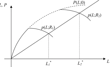
Combining Proposition 2 with Corollary 1 shows how shifts in monetary policy influence the indirect pricing function. This is illustrated in Figure 1 which presents the impact of an increase in the supply of funds from R1 to R2. By Proposition 2, the pricing function p(L;R) is identical to the function P(L,0) up to the point ¯B(R), after which for anyL >B¯(R) it is decreasing. As can be seen in the figure, P(L,0) therefore serves as an envelope of p(L;R): for any R, the two functions are equal up to the point ¯B(R), whileP(L,0) is greater thanp(L;R) forL greater than
¯
B(R).
4.2. Monetary Policy, Liquidation Values, and Lending
In this section we characterize the impact of monetary policy on lending, collateral values, and interest rates when the value of assets is determined endogenously. We will say that monetary policy is ‘effective atR’ if, in equilibrium, when loan supply is equal toR, the entire loan supply is lent out. Alternatively, monetary policy is ‘ineffective at R’ if when loan supply is equal to R, an amount strictly less thanR is lent out in equilibrium. We begin with the following proposition. Proposition 3. Consider a loan supply R. Banks can lend out R in loans in equilibrium if and only ifP( ¯B(R),0)≥B¯(R). Consequently, monetary policy is effective at a loan supplyR= ¯B−1(L) if and only ifP(L,0)≥L.
Proposition 3 is quite intuitive. First, the minimal level of collateral required to extract R in loans is ¯B(R). To see this note that if the value of collateral,L, is less than ¯B(R), since no firm can borrow more thanL, the marginal firm able to borrow will have borrowing requirementB <B¯(R). By definition of ¯B(R), this then implies that aggregate loan supply lent out will be smaller thanR. Second, themaximal value of collateral when R is lent out isP( ¯B(R),0). This is because when R
is lent out the marginal firm obtaining financing will have a borrowing requirement of ¯B(R), and liquidity is highest when the interest rate is zero. Proposition 3 states that if the maximal value of collateral conditional on R being lent out – i.e. P( ¯B(R),0) – is smaller than the minimal amount of collateral required to extract R – i.e. ¯B(R) – then R will not be lent out. In contrast, R will be lent out if the maximal value of collateral associated withR being lent out is greater than the 20This effect is similar to the analysis of Diamond and Rajan (2001) which shows that an adverse effect of liquidity provision is to raise real interest rates which may lead to more bank failures and lower subsequent aggregate liquidity.
minimal value of collateral required to extract R. In this case, the equilibrium interest rate and liquidation value will adjust to equate effective loan demand to loan supply,R.
Using Proposition 2 and Proposition 3, we can analyze the general equilibrium effects of shifts in the supply of loanable funds. Proposition 4 provides a formal characterization of three types of equilibria that arise.
Proposition 4. Consider the pricing functionP(L,0).
(i) The conventional equilibrium: If P(L,0) > L for all 0 ≤ L ≤ I then aggregate lending increases one-for-one with increases in the loan supply R on the range 0 ≤ R ≤ Rmax, where
Rmax =
I
0 BdG(B) is the maximal level possible of aggregate lending. Monetary policy is there-fore effective at any level of reserves R≤Rmax. Further, in this region the equilibrium liquidation
value of assets is increasing in loan supplyR.
(ii) The credit trap equilibrium: Assume that P(L,0) is concave in L, with P(L∗,0) = L∗,
P(L,0)> Lfor 0≤L < L∗, and P(L,0)< L forL > L∗. Then monetary policy is effective up to the loan supply R∗= ¯B−1(L∗) and ineffective beyondR∗. Increases in loan supply beyond R∗ do not increase lending, nor do they change the equilibrium liquidation value of assets which remains constant at L∗. Maximal aggregate lending is therefore R∗ and the maximal liquidation value of assets isL∗.
(iii)The jump-start equilibrium: Assume that P(L,0) is convex inL over the region [L1,L2], with P(Li,0) = Li for i=1,2, P(L,0) > L for 0 ≤ L < L1, and P(L,0) < L for L1 < L < L2. Then, monetary policy is ineffective over the region (R1, R2), whereRi = ¯B−1(Li) (i=1,2), but is effective at loan supplyR2. Further, increases in loan supply over the region [R1, R2) do not change the equilibrium liquidation value which remains constant at L1. However, L2 is an equilibrium liquidation value at loan supplyR2.
Proof. In the Appendix.
Conventional Equilibrium
First, consider the conventional equilibrium in case (i). Since P(L,0) > L for all 0 ≤ L ≤ I, Proposition 3 directly implies that any loan supplyR can be lent out, up to the maximal possible level of lending,Rmax=0IBdG(B). Monetary policy in this equilibrium is therefore fully effective: increases inR are matched one to one with increases in aggregate lending, up toRmax.
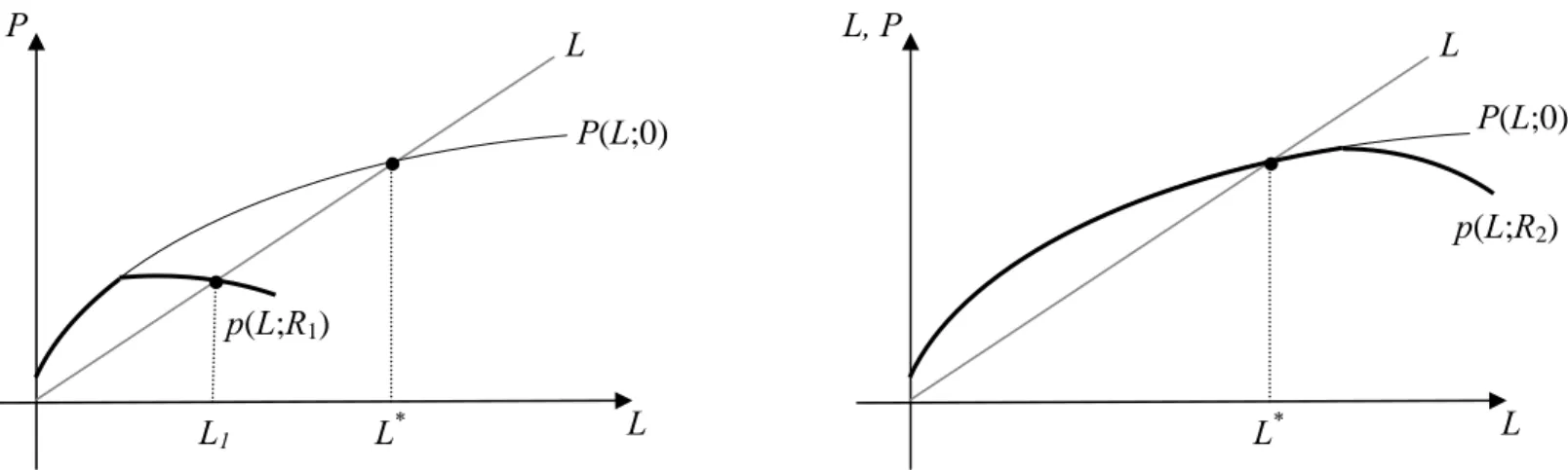
Figure 2 demonstrates this conventional equilibrium. Increases inRshift out the indirect pricing function p(L;R) as described in Proposition 2. This shift in p(L;R) implies that the equilibrium liquidation value – i.e. the price of assets – will increase (fromL∗1 toL∗2 in the figure). The overall chain of events of an increase in loan supply can then be summarized as follows: The increased loan supply is lent out to the corporate sector; the increased liquidity in the corporate sector increases collateral values; and finally, the increase in collateral values increases firm debt capacity, thereby enabling the increase in loan supply.
The effect on equilibrium interest rates of a shift in loan supply is less clear cut. This is best demonstrated in Figure 3 which graphs loan supply and loan demand as a function of interest rates,
r. The main point is thateffective demand for loans is not just a function of the loan interest rate, but is also influenced by collateral values. Firm borrowing in the model is determined both by their desire to borrow as well as their ability to do so. Loan demand can thus be represented by the functionD(r;L∗), where L∗ is the equilibrium collateral price.
As can be seen in Figure 3, an increase in R has two effects. First, loan supply shifts out. Second, effective loan demand shifts out as well – equilibrium liquidation values increase, thereby increasing firm borrowing capacity. While the outward shifts in loan supply and loan demand both push aggregate lending upwards, they have countervailing effects on the equilibrium interest rate. If loan demand shifts out sufficiently – due to a large increase in collateral prices – the change in the equilibrium interest rate will be small.21 Put differently, in a conventional equilibrium large changes in aggregate lending and investment can be associated with small changes in interest rates. This is consistent with evidence that monetary shocks have large real effects, even though empirical studies show that components of aggregate spending are not very sensitive to cost-of-capital variables (see e.g. Blinder and Maccini(1991)).
21In fact, the equilibrium interest rate may actually rise with increases in loan supply. Formally, it is easy to show that the condition for this is ∂P( ¯B∂B(R∗),r∗) >1 +r∗. That is, the sensitivity of the value of collateral to changes in
liquidity (as proxied byB∗, the marginal firm obtaining financing) is sufficiently large. We return to this point when discussing jump-start, quantitative easing equilibria.
Credit Trap Equilibrium
Consider now the credit trap equilibrium represented in case (ii) of Proposition 4. In this equilib-rium, monetary policy is ineffective at any point beyondR∗. The intuition is that for any additional loan supply above R∗ to actually be lent out by banks, liquidation values need to be sufficiently high. However, in a credit trap the implied increase in date-1 liquidation values associated with a marginal increase aggregate lending above and beyond R∗ is not sufficient to induce banks to actually lend the additional funds at date-0. Monetary policy thus becomes ineffective above the loan supply R∗.
The equilibrium is depicted in Figure 4. If the central bank sets reserve level at R1 < R∗, there is a positive equilibrium liquidation value – L1 in the figure – in which aggregate lending is
R1. However, monetary policy is completely ineffective at any point beyond R∗. As loan supply increases beyondR∗, say toR2 in the figure, the sole positive equilibrium liquidation value remains at L∗ and equilibrium lending remains constant at R∗. This is because the rate at which the implied value of collateral increases is not sufficiently high to enable banks to lend the additional loan supply. Put differently, banks rationally understand that lending any incremental amount beyond R∗ does not increase collateral values sufficiently to support the additional lending. Since the equilibrium liquidation valueL∗ does not change with increases in loan supply aboveR∗, firm borrowing capacity remains constant. This implies that realized lending remains at R∗ with the differenceR−R∗ invested by banks. Finally, since beyond loan supplyR∗ effective loan demand is smaller than loan supply, based on Theorem 2(i), the equilibrium interest rate will remain constant at zero. Monetary policy is powerless in increasing lending, collateral values or corporate liquidity. To emphasize, note that in this credit trap equilibrium, increased liquidity in the corporate sector would have increased collateral values which could then serve to enable additional lending. The issue, though, is that banks are not willing to supply the additional liquidity on their own. Regardless of the stance of monetary policy, collateral values therefore remain depressed at a low level implied by the lack of liquidity in the corporate sector.22
Jump-start equilibrium
Consider now the jump-start equilibrium of case (iii) in Proposition 4. As exhibited in Figure 5, 22This reasoning suggests that direct injections of liquidity into the corporate sector may be useful – a point we return to in Section 6.
for any loan supply R1 < R < R2, the only equilibrium has a liquidation value of L = L1 and associated lending of R1 = ¯B−1(L1).23 Increases in the loan supply over the region [R1, R2) are therefore completely ineffective in increasing lending and collateral values. There is no response to injections of liquidity by the central bank: the equilibrium liquidation value is stuck at L1 and lending remains constantR1. Further, since as in a credit trap equilibrium, effective loan demand will be depressed due to the low level of liquidation values, in this region the interest rate on loans will be constant at zero, its lower bound.
In contrast, if the central bank acts forcefully enough by increasing loan supply toR2, another equilibrium arises. In this equilibrium the liquidation value of assets is high – L2 in the figure – enabling the full loan supplyR2 to be lent out. This equilibrium arises due to the feedback effect between lending and collateral values: lending is high because collateral values are large enough to support it, while collateral values are high because lending increases liquidity in the corporate sector.
The jump-start equilibrium therefore demonstrates how a policy of quantitative easing may successfully reignite bank lending. Banks know that when loan supply is moderate, the implied value of collateral conditional on lending occurring is not high enough to actually justify lending. However, when loan supply is expanded sufficiently, a new high lending and high collateral value rational expectations equilibrium arises.
It should be emphasized that although a new equilibrium arises with a sufficiently forceful monetary expansion, it is by no means clear that banks will successfully coordinate on it. If each bank assumes that the others will continue lending at depressed levels, the economy will be stuck in the inefficient equilibrium. In this sense, a policy of quantitative easing in and of itself may not be sufficient to jump-start lending and collateral values. The central bank, or more generally government at large, may require other tools to solve the coordination problem arising between banks.24
The jump-start equilibrium also explains how small contractions in the stance of monetary policy can lead to large crashes in asset values and lending. This is simply the flip-side of quantitative easing. Returning to Figure 5, consider an economy with loan supply at R2 and liquidation value 23To see this note that for anyRin this region, the only value wherep(L;R) equals LisL=L1. Further, in this regionP( ¯B(R),0)<B¯(R) which by Proposition 3 implies thatR will not be lent out.
24To eliminate the low lending equilibrium, these actions may include government subsidies for new loans, a tax on bank reserves, or government prodding to increase lending (as seen, for example, during the crisis of 2008-2009).
atL2. An incremental reduction in loan supply fromR2 leads to a collapse in lending and collateral values to R1 and L1, respectively. The small reduction in lending reduces liquidity and collateral values, which in turn reduces liquidity further. The negative feedback effect between lending, liquidity and collateral values drives all three to lower levels until the process stops at the new equilibrium.
Interestingly, the monetary contraction will also reduce the interest rates (to zero according to Proposition 2). The intuition is that while loan supply decreases by a small amount, effective loan demand collapses because of the attendant drop in collateral values. A form of flight to quality arises in which the supply of loans is distributed at low cost to the comparatively small number of firms that have balance sheets strong enough to borrow.
Taken together, therefore, in this equilibrium monetary contraction can lead to crashes in lending and collateral values coupled with a reduction in interest rates. These effects are very much consistent with accounts of the Japanese experience during the 1980s such as Bernanke and Gertler (1995) who argue that “the crash of Japanese land and equity values in the latter 1980s was the result (at least in part) of monetary tightening; ... [T]his collapse in asset values reduced the creditworthiness of many Japanese corporations and banks, contributing to the ensuing recession.” To conclude, Proposition 4 shows that the efficacy of monetary policy crucially depends on the shape and level of the pricing function P – i.e. on how collateral prices vary with corporate liquidity. A low and concave pricing function will generally lead to a credit trap equilibrium where quantitative easing will be ineffective in increasing lending and liquidation values, regardless of the level of loan supply set by the central bank. In contrast, convexities in the pricing function will lead to a jump start equilibrium where quantitative easing may be useful. What determines the shape of the pricing function – and hence the efficacy of quantitative easing – is therefore a natural question which we turn to in the next section.
5.
Microfoundations of the Collateral Pricing Function
In this section we impose more structure on the pricing function of assets,P, by building micro-founded models of collateral values and the market for assets. In the first model, collateral values are determined in a competitive market for repossessed assets. The second model involves a bar-gaining setting in which, when selling repossessed assets, the bank negotiates a price with a limited
set of potential buyers. Finally, we show that search costs associated with finding a suitable buyer for assets introduces convexities in the pricing function and hence the possibility of a jump-start, quantitative easing equilibrium.
A Competitive Market for Repossessed Assets
Consider the case where the price of collateral is determined in a competitive market in which the equilibrium price of assets at date-1 is set so as to equate the demand and supply of assets. We assume that firms that invested at date zero – which we call industry insiders – develop the know-how to operate assets of firms liquidated at date 1. Operating liquidated assets enables these firms to generate cash flow V with V < X2 at date 2.25 For ease of exposition, we further assume that V > X1. Since X1 is the maximal wealth of firms in the economy, this assumption implies that at date-1 firms will be willing to pay their full internal wealth to obtain liquidated assets.26
Aside from demand stemming from industry insiders, we assume that there is a perfectly elastic supply of capital at date-1 ready to buy liquidated assets at a positive price of kV < X1. This supply of capital should be thought of as stemming from industry outsiders who can employ the assets but only in an inferior use.
Finally, we assume that at date-1, a supply α of assets, exogenous to the model, are sold on the market. Variations in α capture shifts in the supply of assets which must be cleared in the market.27 For example, in a downturn the supply of assets sold on the market will be high.
To obtain the pricing function P(L,0), we calculate for every L the market clearing price of assets assuming that (a) the marginal borrowing firm has a date-0 borrowing requirement ofLand (b) the interest rate on loans is zero. To do this, for every Lwe calculate the demand schedule for assets and equate it to asset supply α.
Consider first anyLthat is sufficiently small to satisfykV ≤X1−L. Note that if the marginal borrowing firm has a date-0 borrowing requirement ofL, the date-1 wealth distribution of industry insiders – i.e. those that invested – will have a support of [X1−L, X1].28 This implies that at any priceP ≤X1−Lall industry insiders will be able to purchase assets. Since their aggregate date-1 wealth is0L(X1−B)dG(B), the demand for assets at any priceP ∈[kV, X1−L] is given by
25Liquidation is inefficient in that the industry insider purchasing the assets is a second-best user: V < X2. 26Assuming thatV < X1 generates similar results, but the pricing function developed below is capped atV. 27At the cost of additional complexityαitself could be endogenized to capture the number of firms experiencing liquidity defaults.
D(P;L) = ⎧ ⎨ ⎩ L 0 (X1−B)dG(B) P if P ∈(kV,≤X1−L] D s.t. D≥ L 0 (X1−B)dG(B) kV if P =kV (9)
Note that since industry outsiders are ready to purchase any amount of assets at a price ofP =kV, demand at this price is perfectly elastic at any quantity greater than
L
0 (X1−B)dG(B)
kV , the demand
stemming from industry insiders.29
In contrast, for any priceP ∈(X1−L, X1], firms require a date-1 wealth of at leastP to purchase assets. This implies that demand over this range will be
D(P;L) =
X1−P
0 (X1−B)dG(B)
P (10)
Taken together, (9) and (10) define the demand scheduleD(P;L) for anyLsatisfyingkV ≤X1−L. On the other hand, forLsatisfyingkV > X1−L, it is easy to see that demand is given solely by (10) with the addition that atP =kV demand is perfectly elastic above
X1−kV
0 (X1−B)dG(B)
kV .
For any L, the equilibrium price of assets solves D(P;L) = α, equating demand and supply. By definition, this equilibrium price is equal toP(L,0). The following corollary characterizes this pricing function (see Figure 6):
Corollary 2. For any α <
X1−kV 0 (X1−B)dG(B) kV , define L∗1(α) implicitly by L∗1(α) 0 (X1−B)dG(B) kV =α.
Further, define L∗2(α) implicitly by
L∗2(α)
0 (X1−B)dG(B)
X1−L∗2(α) = α. Then the pricing function P(L,0)
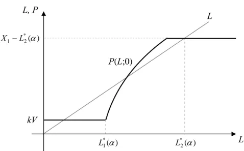
satisfies P(L,0) = ⎧ ⎪ ⎨ ⎪ ⎩ kV if L≤L∗1(α) (α1)0L(X1−B)dG(B) if L∗1(α)< L≤L∗2(α) X1−L∗2(α) if L > L∗2(α)
Further, M axL{P(L,0)}=X1−L∗2(α) is strictly greater than the outside valuation kV. Proof. See Appendix.
To understand Corollary 2, note that as L increases, more firms obtain financing, thereby increasing date-1 liquidity available to purchase assets. However, ifLis comparatively low – and in particular, smaller thanL∗1(α) – aggregate liquidity of industry insiders is not sufficient to clear the market for assets. The marginal buyers, therefore, are industry outsiders, implying that the market
clearing price is kV.30 As L increases beyond L∗1(α), industry-insider aggregate liquidity becomes sufficiently large to enable them to become the marginal buyers of assets. In this region, increases in
Lshift out the demand schedule for assets of industry insiders, implying that the price of collateral will increase as well. Finally, beyond L∗2(α), increases in L do not affect the equilibrium price of assets which remains constant atX1−L∗2(α). At this price, aggregate liquidity is large enough to clear the entire supply of assets. Further increases in the liquidation valueL do increase aggregate liquidity, but only by adding firms with internal wealth lower than the priceX1 −L∗2(α). Thus, even though there are more potential buyers, the equilibrium price remains constant atX1−L∗2(α). It is easy to see that at any exogenousL, the pricing functionP(L,0) is decreasing inα: Since the demand for assets is determined by (the finite) available date-1 liquidity and is not perfectly elastic at the fundamental value V, the price must drop to clear the market. This yields the following proposition:
Proposition 5. For any outside value kV < X1
2 , there exists an α <¯
X1−kV
0 (X1−B)dG(B) kV , such
that for any α >α¯, regardless of the stance of monetary policy, the equilibrium value of collateral will bekV and aggregate lending will equal B¯−1(kV).
Proof. See Appendix.
Proposition 5 shows how expectations of asset sales inhibit the effectiveness of monetary policy. Anticipating a large number of assets on the market, banks understand that the price of collateral will be low. As in a credit trap, while lending would have served to increase date-1 liquidity and with it the price of collateral, the implied value of collateral is too small to actually justify the lending. The economy therefore suffers from a lack of liquidity, collateral prices are depressed at liquidity pricing levels, and lending remains low regardless of the stance of monetary policy.
To emphasize, because ¯α ≤
X1−kV
0 (X1−B)dG(B)
kV , as Corollary 2 shows the collateral pricing
function P(L,0) does increases beyond the outside-valuation of kV (see Figure 6). However, to enable the value of collateral to increase beyond kV, banks need to supply liquidity to industry insiders, increasing their liquidity sufficiently so that they, rather than the industry outsiders, are the marginal buyers of asset. This, however, will not occur. Regardless of the stance of monetary policy, banks will not lend any level of loan supply greater than ¯B−1(kV) since the implied value of
30Indeed, whenα >0X1−kV(X1−B)dG(B)
kV , it is easy to show thatP(L,0) equalskV for allL. Since asset supply is comparatively large, the marginal buyer will always be an industry outsider.