Zurich Open Repository and Archive University of Zurich Main Library Strickhofstrasse 39 CH-8057 Zurich www.zora.uzh.ch Year: 2018
Really uncertain business cycles
Bloom, Nicholas ; Floetotto, Max ; Jaimovich, Nir ; Saporta-Eksten, Itay ; Terry, Stephen J
Abstract: We investigate the role of uncertainty in business cycles. First, we demonstrate that microe-conomic uncertainty rises sharply during recessions, including during the Great Recession of 2007–2009. Second, we show that uncertainty shocks can generate drops in gross domestic product of around 2.5% in a dynamic stochastic general equilibrium model with heterogeneous firms. However, we also find that uncertainty shocks need to be supplemented by first‐moment shocks to fit consumption over the cycle. So our data and simulations suggest recessions are best modelled as being driven by shocks with a nega-tive first moment and a posinega-tive second moment. Finally, we show that increased uncertainty can make first‐moment policies, like wage subsidies, temporarily less effective because firms become more cautious in responding to price changes.
DOI: https://doi.org/10.3982/ECTA10927
Posted at the Zurich Open Repository and Archive, University of Zurich ZORA URL: https://doi.org/10.5167/uzh-151988
Journal Article Published Version
Originally published at:
Bloom, Nicholas; Floetotto, Max; Jaimovich, Nir; Saporta-Eksten, Itay; Terry, Stephen J (2018). Really uncertain business cycles. Econometrica, 86(3):1031-1065.
Econometrica, Vol. 86, No. 3 (May, 2018), 1031–1065
REALLY UNCERTAIN BUSINESS CYCLES NICHOLASBLOOM
Dept. of Economics, Stanford University
MAXFLOETOTTO McKinsey & Company
NIRJAIMOVICH
Dept. of Economics, University of Zurich
ITAYSAPORTA-EKSTEN
Dept. of Economics, Tel Aviv University and Dept. Economics, University College London
STEPHENJ. TERRY Dept. of Economics, Boston University
We investigate the role of uncertainty in business cycles. First, we demonstrate that microeconomic uncertainty rises sharply during recessions, including during the Great Recession of 2007–2009. Second, we show that uncertainty shocks can generate drops in gross domestic product of around 2.5% in a dynamic stochastic general equilibrium model with heterogeneous firms. However, we also find that uncertainty shocks need to be supplemented by first-moment shocks to fit consumption over the cycle. So our data and simulations suggest recessions are best modelled as being driven by shocks with a negative first moment and a positive second moment. Finally, we show that in-creased uncertainty can make first-moment policies, like wage subsidies, temporarily less effective because firms become more cautious in responding to price changes.
KEYWORDS: Uncertainty, adjustment costs, business cycles.
1. INTRODUCTION
UNCERTAINTYhas received substantial attention recently. For example, the Federal Open
Market Committee minutes repeatedly emphasize uncertainty as a key factor in the 2001 and 2007–2009 recessions. This paper seeks to evaluate the role of uncertainty for busi-ness cycles in two parts. In the first part, we develop new empirical measures of uncer-tainty using detailed Census microdata from 1972–2011 and we highlight three main results. First, the dispersion of plant-level innovations to their total factor productivity (TFP) is strongly countercyclical, rising steeply in recessions. For example, Figure1shows the dispersion of TFP shocks for a balanced panel of plants during the 2 years before the Great Recession (2005–2006) and 2 years during the recession (2008–2009). We find
Nicholas Bloom:[email protected]
Max Floetotto:[email protected] Nir Jaimovich:[email protected]
Itay Saporta-Eksten:[email protected] Stephen J. Terry:[email protected]
Any opinions and conclusions expressed herein are those of the authors and do not necessarily represent the views of the U.S. Census Bureau. All results have been reviewed to ensure that no confidential information is disclosed. We thank our editor Lars Hansen, our anonymous referees, our formal discussants Sami Alpanda, Eduardo Engel, Frank Smets, Eric Swanson, and Iván Alfaro, as well as Angela Andrus at the RDC and numerous seminar audiences for comments.
1032 BLOOM ET AL.
FIGURE1.—The variance of establishment-level TFP shocks increased by 76% in the Great Recession. Notes: Constructed from the Census of Manufactures and the Annual Survey of Manufactures using a bal-anced panel of 15,752 establishments active in 2005–2006 and 2008–2009. TFP Shocks are defined as residuals from a plant-level log(TFP)AR(1) regression that also includes plant and year fixed effects. Moments of the distribution for non-recession (recession) years are: mean 0 (−0166), variance 0.198 (0.349), coefficient of skewness−1060 (−1340) and kurtosis 15.01 (11.96). The year 2007 is omitted because according to the NBER the recession began in 12/2007, so 2007 is not a clean “before” or “during” recession year.
that plant-level TFP shocks increased in variance by 76% during the recession. Similarly, Figure 2shows that the dispersion of output growth for these same establishments in-creased even more, rising by a striking 152% during the recession. Thus, as Figures1and 2suggest, recessions appear to be characterized by a negative first-moment and a positive second-moment shock to the establishment-level driving processes.
Our second empirical finding is that uncertainty is also strongly countercyclical at the industry level. That is, at the Standard Industrial Classification (SIC) four-digit industry level, the yearly growth rate of output is negatively correlated with the dispersion of TFP shocks to establishments within the industry. Hence, both at the industry and at the ag-gregate level, periods of low growth rates of output are also characterized by increased cross-sectional dispersion of TFP shocks.
Our third empirical finding is that for plants owned by publicly traded Compustat ent firms, the size of their plant-level TFP shocks is positively correlated with their par-ents’ daily stock returns. Hence, daily stock returns volatility—a popular high-frequency financial measure of uncertainty that also rises in recessions—is tightly linked to the size of yearly plant TFP shocks.
Given this empirical evidence that uncertainty appears to rise sharply in recessions, in the second part of the paper we build a dynamic stochastic general equilibrium (DSGE) model. Various features of the model are specified to conform as closely as possible to the standard frictionless real business cycle (RBC) model as this greatly simplifies compari-son with existing work. We deviate from this benchmark in three ways. First, uncertainty is time-varying, so the model includes shocks to both the level of technology (the first moment) and its variance (the second moment) at both the microeconomic and macroe-conomic levels. Second, there are heterogeneous firms that are subject to idiosyncratic shocks. Third, the model contains nonconvex adjustment costs in both capital and labor.
UNCERTAIN BUSINESS CYCLES 1033
FIGURE2.—The variance of establishment-level sales growth rates increased by 152% in the Great Reces-sion. Notes: Constructed from the Census of Manufactures and the Annual Survey of Manufactures using a balanced panel of 15,752 establishments active in 2005–2006 and 2008–2009. Moments of the distribution for non-recession (recession) years are: mean 0.026 (−0191), variance 0.052 (0.131), coefficient of skewness 0.164 (−0330) and kurtosis 13.07 (7.66). The year 2007 is omitted because according to the NBER the recession began in 12/2007, so 2007 is not a clean “before” or “during” recession year.
The nonconvexities together with time variation in uncertainty imply that firms become more cautious in investing and hiring when uncertainty increases.
The model is numerically solved and estimated using macro- and plant-level data via a simulated method of moments (SMM) approach. Our SMM parameter estimates suggest that micro- and macro-uncertainty increase by around threefold during recessions.
Simulations of the model allow us to study its response to an uncertainty shock. In-creased uncertainty makes it optimal for firms to wait, leading to significant falls in hir-ing, investment, and output. In our model, overall, uncertainty shocks generate a drop in gross domestic product (GDP) of around 2.5%. Moreover, the increased uncertainty re-duces productivity growth. This reduction occurs because uncertainty rere-duces the degree of reallocation in the economy since productive plants pause expanding and unproduc-tive plants pause contracting. The importance of reallocation for aggregate productivity growth matches empirical evidence in the United States. See, for example,Foster, Halti-wanger, and Krizan(2000, 2006), who report that reallocation broadly defined accounts for around 50% of manufacturing and 80% of retail productivity growth in the United States.
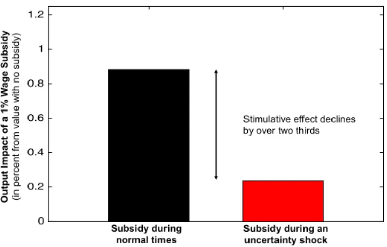
We then build on our theoretical model to investigate the effects of uncertainty on policy effectiveness. We use a simple illustrative example to show how time-varying un-certainty initially dampens the effect of an expansionary policy. The key to this policy ineffectiveness is that a rise in uncertainty makes firms cautious in responding to any stimulus.
Our work is related to several strands in the literature. First, we add to the extensive literature building on the DSGE framework that studies the role of TFP shocks in caus-ing business cycles. In this literature, recessions are generally caused by large negative technology shocks (e.g.,King and Rebelo (1999)). The reliance on negative technology shocks has proven to be controversial, as it suggests that recessions are times of
techno-1034 BLOOM ET AL.
logical regress. As discussed above, our work provides a rationale for at least some portion of variation in measured productivity. Countercyclical increases in uncertainty lead to a freeze in economic activity, substantially lowering productivity growth during recessions.
Second, the paper relates to the literature on investment under uncertainty. A rapidly growing body of work has shown that uncertainty can directly influence firm-level invest-ment and employinvest-ment in the presence of adjustinvest-ment costs. Recently, the literature has started to focus on stochastic volatility and its impacts on the economy.1Finally, the
pa-per also builds upon a recent literature that studies the role of microeconomic rigidities in general equilibrium macromodels.2
The remainder of this paper is organized as follows. Section 2 discusses the empiri-cal behavior of uncertainty over the business cycle. In Section3, we formally present the DSGE model, define the recursive equilibrium, and present our nonlinear solution al-gorithm. We discuss the estimation of parameters governing the uncertainty process in Section 4, while in Section5, we study the impact of uncertainty shocks on the aggre-gate economy. Section6studies the implications for government policy in the presence of time-varying uncertainty. Section7concludes. Appendixes in the Supplementary Ma-terial (Bloom, Floetotto, Jaimovich, Saporta-Eksten, and Terry (2018)) include details on the data (Appendix A), model solution (Appendix B), estimation (Appendix C), and a benchmark representative agent model (Appendix D).
2. MEASURING UNCERTAINTY OVER THE BUSINESS CYCLE
Before presenting our empirical results, it is useful to briefly discuss what we mean by time-varying uncertainty in the context of our model.
We assume that a firm, indexed by j, produces output in period t according to the production function
yjt=Atzjtf (kjt njt) (1)
wherektjandntjdenote idiosyncratic capital and labor employed by the firm. Each firm’s
productivity is a product of two separate processes: an aggregate component,At, and an
idiosyncratic component,zjt.
We assume that the aggregate and idiosyncratic components of business conditions fol-low autoregressive (AR) processes:
log(At)=ρAlog(At−1)+σtA−1εt (2)
log(zjt)=ρZlog(zjt−1)+σtZ−1εjt (3)
1For a focus on the firm level, seeBernanke(1983),Romer(1990),Bertola and Caballero(1994),Dixit and Pindyck(1994),Abel and Eberly(1996),Hassler(1996), andCaballero and Engel(1999). For a macro-focus, seeBloom’s (2009) partial equilibrium model with stochastic volatility, Fernandez-Villaverde, Guerron-Quintana, Rubio-Ramirez, and Uribe’s (2011) paper on uncertainty and real exchange rates,Kehrig’s (2015) paper on countercyclical productivity dispersion,Christiano, Motto, and Rostagno’s (2014),Arellano, Bai, and Kehoe’s (2012), and Gilchrist, Sim, and Zakrajsek’s (2014) papers on uncertainty shocks in models with finan-cial constraints,Basu and Bundick’s (2016) paper on uncertainty shocks in a new-Keynesian model, Fernandez-Villaverde, Guerron-Quintana, Kuester, and Rubio-Ramirez’s (2015) paper on fiscal policy uncertainty, and Bachmann and Bayer’s (2013, 2014) papers on microlevel uncertainty with capital adjustment costs.
2See, for example, Hopenhayn and Rogerson (1993), Thomas (2002), Veracierto (2002), Gourio and Kashyap (2007),Khan and Thomas(2008, 2013),Bachmann, Caballero, and Engel(2013),House (2014), orWinberry(2016).
UNCERTAIN BUSINESS CYCLES 1035 We allow the variance of innovations,σA
t andσ
Z
t , to move over time according to
two-state Markov chains, generating periods of low and high macro- and micro-uncertainty. There are two assumptions embedded in this formulation. First, the volatility in the idiosyncratic component, zjt, implies that productivity dispersion across firms is
time-varying, while volatility in the aggregate component,At, implies thatallfirms are affected
by more volatile shocks. Second, given the timing assumption in (2) and (3), firms learn in advance that the distribution of shocks from which they will draw in the next period is changing. This timing assumption captures the notion of uncertainty that firms face about future business conditions.
These two shocks are driven by different statistics. Volatility inzjt implies that
cross-sectional dispersion-based measures of firm performance (output, sales, stock market re-turns, etc.) are time-varying, while volatility inAt induces higher variability in aggregate
variables like GDP growth and the Standard and Poor’s 500 index. Next we turn to our cross-sectional and macroeconomic uncertainty measures, detailing how both appear to rise in recessions.
2.1. Microeconomic Uncertainty Over the Business Cycle
In this section we present a set of results showing that shocks at theestablishment-level,
firm-level, and industry-level all increase in variance during recessions. In our model in Section3we focus on units of production, ignoring multi-establishment firms or industry-level shocks to reduce computational burden. Nevertheless, we present data at these three different levels to demonstrate the generality of the increase in idiosyncratic shocks dur-ing recessions.
Our first set of measures comes from the Census panel of manufacturing establish-ments. In summary, with extensive details in Appendix A, this data set contains de-tailed output and input data on over 50,000 establishments from 1972 to 2011. We focus on the subset of 15,673 establishments with 25+ years of data to ensure that compo-sitional changes do not bias our results, generating a sample of almost half a million establishment–year observations.
To measure uncertainty, we first calculate establishment-level TFP (zjt) using the
stan-dard approach fromFoster, Haltiwanger, and Krizan(2000). We then define TFP shocks (ejt) as the residual from the first-order autoregressive equation for establishment-level
log TFP,
log(zjt)=ρlog(zjt−1)+µj+λt+ejt (4)
whereµj is an level fixed effect (to control for permanent
establishment-level differences) andλt is a year fixed effect (to control for cyclical shocks). Since this
residual also contains plant-level demand shocks that are not controlled for by four-digit price deflators (seeFoster, Haltiwanger, and Syverson(2008)), our revenue-based mea-sure will combine both TFP and demand shocks.
Finally, we define microeconomic uncertainty,σZ
t−1, as the cross-sectional dispersion of
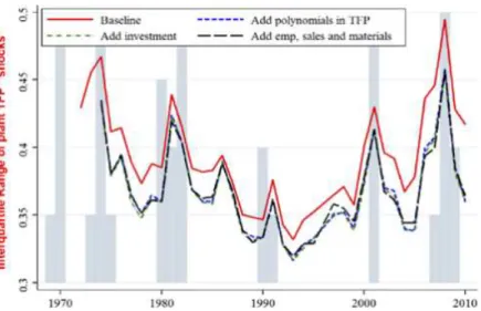
ejtcalculated on a yearly basis. In Figure3, we depict the interquartile range (IQR) of this
TFP shock within each year. As Figure3shows, the series exhibits a clearly countercyclical behavior. This is particularly striking for the recent Great Recession of 2007–2009, which displays the highest value of TFP dispersion since the series began in 1972.
TableImore systematically evaluates the relationship between the dispersion of TFP shocks and recessions. In column 1, we regress the cross-sectional standard deviation (S.D.) of establishment TFP shocks on an indicator for the number of quarters in a re-cession during that year. So, for example, this variable has a value of 0.25 in 2007 as the
1036 BLOOM ET AL.
FIGURE3.—TFP “shocks” are more dispersed in recessions. Notes: Constructed from the Census of Man-ufactures and the Annual Survey of ManMan-ufactures establishments, using establishments with 25+years to address sample selection. Grey shaded columns are the share of quarters in recession within a year.
recession started in quarter IV, and values of 1 and 0.5 in 2008 and 2009, respectively, as the recession continued until quarter II in 2009. We find a coefficient of 0.064, which is highly significant (at-statistic of 6.9). Given that the mean of the S.D. of establishment TFP shocks is 0.503, a year in recession is associated with a 13% increase in the dispersion of TFP shocks. In the bottom panel, we report that this S.D. of establishment TFP shocks also has a highly significant correlation with GDP growth of−045.
Our finding here of countercyclical dispersion of microlevel outcomes mirrors a range of other recent papers such as Bachmann and Bayer (2014) in German data, Kehrig (2015) in a similar sample of U.S. Census data, orJurado, Ludvigson, and Ng (2014), Vavra(2014), andBerger and Vavra(2015) for different samples of U.S. firms. A num-ber of these papers build alternative theories or interpretations of such patterns in the microdata qualitatively distinct from our own, but the core empirical regularity of coun-tercyclical microlevel dispersion is remarkably robust.
In columns 2 and 3, we examine the coefficient of skewness and kurtosis of TFP shocks over the cycle and, interestingly, find no significant correlations.3This suggests that
reces-sions can be characterized at the microeconomic level as a negative first-moment shock plus a positive second-moment shock. In column 4, we use an outlier-robust measure of cross-sectional dispersion, which is the IQR range of TFP shocks, and again find this rises significantly in recessions. The point estimate on recession of 0.061 implies an increase of over 15% in the IQR of TFP shocks in a recession year.4In column 5, as another
robust-3This lack of significant correlation was robust in a number of experiments we ran. For example, if we drop the time trend and Census survey year controls, the result in column 1 on the standard deviation remains highly significant at 0.062 (0.020), while the results in columns 2 and 3 on skewness and kurtosis remain insignificant at−0250 (0.243) and−0771 (2.755). We also experimented with changing the establishment selection rules (keeping those with 2+or 38+years rather than 25+years) and again found the results robust, as shown in Appendix Table A1. Interestingly,Guvenen, Ozkan, and Song(2014) find an increase in left-skewness for personal income growth during recessions, which may be absent in plant data because large negative draws lead plants to exit. Because the drop in the left tail is the key driver of recessions in our model (the “bad news principle” highlighted byBernanke(1983)), this distinction is relatively unimportant.
4While 15% is a large increase in dispersion, it still greatly understates the increase in uncertainty in reces-sion, because a large share of the dispersion of TFP is associated with measurement error. We formally address
UNCER T A IN BUSINESS CY CLES 1037 TABLE I
UNCERTAINTY ISHIGHERDURINGRECESSIONSa
(1) (2) (3) (4) (5) (6) (7) (8)
Dependent S.D. of log(TFP) Skewness of Kurtosis of IQR of log(TFP) IQR of IQR of IQR of IQR of industrial variable: shock log(TFP) log(TFP) shock output growth sales growth stock returns prod. growth
shock shock
Sample: Plants Plants Plants Plants Plants Public firms Public firms Industries
(manufact.) (manufact.) (manufact.) (manufact.) (manufact.) (all sectors) (all sectors) (manufact.)
Recession 0.064∗∗∗ −0.248 −1.334 0.061∗∗∗ 0.077∗∗∗ 0.032∗∗∗ 0.025∗∗∗ 0.044∗∗∗
(0.009) (0.191) (1.994) (0.019) (0.019) (0.007) (0.003) (0.004)
Mean of dep. var. 0.503 −1.525 20.293 0.395 0.196 0.186 0.104 0.101
Corr. GDP growth −0.450∗∗∗ 0.143 0.044 −0.444∗∗∗ −0.566∗∗∗ −0.275∗∗∗ −0.297∗∗∗ −0.335∗∗∗
Frequency Annual Annual Annual Annual Annual Quarterly Monthly Monthly
Years 1972–2011 1972–2011 1972–2011 1972–2011 1972–2011 1962:1–2010:3 1960–2010 1972–2010
Observations 39 39 39 39 39 191 609 455
Underlying sample 461,232 461,232 461,232 461,232 461,232 320,306 931,143 70,487
aEach column reports a time-series ordinary least squares (OLS) regression point estimate (and standard error below in parentheses) of a measure of uncertainty on a recession indicator. The recession indicator is the share of quarters in that year in a recession in columns 1–5, whether that quarter was in a recession in column 6, and whether the month was in recession in columns 7 and 8. Recessions are defined using the National Bureau of Economic Research (NBER) data. In the bottom panel we report the mean of the dependent variable and its correlation with real GDP growth. In columns 1–5, the sample is the population of manufacturing establishments with 25 years or more of observations in the Annual Survey of Manufactures (ASM) or Census of Manufactures (CM) survey between 1972 and 2009, which contains data on 15,673 establishments across 40 years of data (one more year than the 39 years of regression data since we need lagged TFP to generate a TFP shock measure). We include plants with 25+years to reduce concerns over changing samples. In column 1, the dependent variable is the cross-sectional standard deviation (S.D.) of the establishment-level shock to total factor productivity (TFP). This shock is calculated as the residual from the regression of log(TFP)at yeart+1on its lagged value (yeart), a full set of year dummies, and establishment fixed effects. In column 2, we use the cross-sectional coefficient of skewness of the TFP shock, in column 3, the cross-sectional coefficient of kurtosis, and in column 4, the cross-sectional interquartile range of this TFP shock as an outlier robust measure. In column 5, the dependent variable is the interquartile range of plants’ sales growth. In column 6, the dependent variable is the interquartile range of firms’ sales growth by quarter for all public firms with 25 years (100 quarters) or more in Compustat between 1962 and 2010. In column 7, the dependent variable is the within firm-quarter interquartile range of firms’ monthly stock returns for all public firms with 25 years (300 months) or more in Center for Research in Security Prices (CRSP) between 1960 and 2010. Finally, in column 8, the dependent variable is the interquartile range of industrial production growth by month for manufacturing industries from the Federal Reserve Board’s monthly industrial production database. All regressions include a time trend and for columns 1–5 Census year dummies (for Census year and for three lags). Robust standard errors are applied in all columns to control for any potential serial correlation.∗∗∗denotes 1% significance,∗∗denotes 5% significance, and∗denotes 10% significance. Results are also robust to using Newey–West corrections for the standard errors. Data are available athttp://www.stanford.edu/~nbloom/RUBC.zip.
1038 BLOOM ET AL.
ness test, we use plant-level output growth, rather than TFP shocks, and find a significant rise in recessions. We also run a range of other experiments on different indicators, mea-sures of TFP, and samples, and always find that dispersion rises significantly in recessions.5
For example, Figure A1 plots the correlation of plant TFP rankings between consecutive years. This shows that during recessions these rankings churn much more, as increased microeconomic variance leads plants to change their position within their industry-level TFP rankings more rapidly.
In column 6, we use a different data set that is the sample of all Compustat firms with 25+years of data. This has the downside of being a much smaller selected sample con-taining only 2465 publicly quoted firms, but spanning all sectors of the economy, and providing quarterly sales observations going back to 1962. We find that the quarterly dis-persion of sales growth in this Compustat sample is also significantly higher in recessions. One important caveat when using the variance of productivity “shocks” to measure un-certainty is that the residualejt is a productivity shock only in the sense that it is
unfore-casted by the regression equation (4), rather than unforeunfore-casted by the establishment. We address this concern in two ways. First, in column 7 we examine the cross-sectional spread of stock returns, which reflects the volatility of news about firm performance, and again find this is countercyclical, echoing the prior results in Campbell, Lettau, Malkiel, and Xu(2001). In fact, as we discuss below in TableIII, we also find that establishment-level shocks to TFP are significantly correlated to their parent’s stock returns, so that at least part of these establishment TFP shocks are new information to the market. Furthermore, to remove the forecastable component of stock returns, we repeated the specification in column 7 by first removing the quarter by firm mean of firm returns. This controls for any quarterly factors—like size, market/book value, research and development (R&D) in-tensity, and leverage—that may influence expected stock returns (e.g.,Bekaert, Hodrick, and Zhang(2012)), although of course the influence of common factors that may vary at a higher frequency within the quarter may remain. The coefficient (standard error) on recession in these regressions is 0.019 (0.003), similar to the results obtained in column 7. Second, we extend the TFP forecast regressions (4) to include additional observables that are likely to be informative about future TFP changes. Adding these in the regression accounts for at least some of the superior information that the establishment might have over the econometrician, helping us to back out true shocks to TFP from the perspec-tive of the establishments. Figure4reports the IQR of the TFP shocks for the baseline forecast regression, as well as for three other dispersion measures, where we sequentially add more variables to the forecasting regressions that are used to recover TFP shocks. First we add two extra lags in levels and polynomials of TFP, next we also include lags and polynomials of investment, and finally we include lags and polynomials of multiple inputs including employment, energy, and materials expenditure. As is clear from the fig-ure, even when forward looking establishment choices for investment and employment are included, the overall cyclical patterns of uncertainty are almost unchanged.
that in our SMM estimation framework. See Section4.2for estimates of the underlying increase in uncertainty in recession and see Appendix C for details.
5For example, the IQR of employment growth rates has a point estimate (standard error) of 0.051 (0.012), the IQR of TFP shocks measured using an industry-by-industry forecasting equation version of (4) has a point estimate (standard error) of 0.064 (0.019), using 2+year samples for the S.D. of TFP shocks, we find a point estimate (standard error) of 0.046 (0.014), and using a balanced panel of 38+year establishments, we find a point estimate (standard error) of 0.075 (0.015). Finally, the IQR of TFP shocks measured after removing firm–year means and then applying (4) has a point estimate (standard error) of 0.028 (0.011), so that dispersion of productivity shocks even across plants within firms rises within recessions.
UNCERTAIN BUSINESS CYCLES 1039
FIGURE4.—Robustness test: different measures of TFP “shocks” are all more dispersed in recessions. Notes: Constructed from the Census of Manufactures and the Annual Survey of Manufactures establishments, using establishments with 25+years to address sample selection. Grey shaded columns are share of quarters in recession within a year. The four lines are:Baseline: Interquartile Range of plant TFP “shocks” (as in Figure3).
Add polynomials in TFP: includes the first, second and third lags of log TFP, and their degree 5 polynomials in the AR regression which is used to recover TFP shocks.Add investment: includes all the controls from the previous specification plus the first, second and third lags of investment rate, and their degree 5 polynomials.
Add emp, sales and materials: includes all the controls from the previous specification plus the second and third lags of log employment, log sales, and log materials, as well as their degree 5 polynomials.
Finally, in column 8, we examine another measure of uncertainty, which is the cross-sectional spread of industry-level output growth rates, finding again that this is strongly countercyclical.
Hence, in summary plant-level (columns 1–5), firm-level (columns 6 and 7), and industry-level (column 8) measures of volatility and uncertainty all appear to be strongly countercyclical, suggesting that microeconomic uncertainty rises in recessions at all levels.
2.2. Industry Business Cycles and Uncertainty
In Table II, we report another set of results that disaggregate down to the industry level, finding a very similar result that uncertainty is significantly higher during periods of slower growth. To do this, we exploit the size of our Census data set to examine the dispersion of productivity shockswithineach SIC four-digit industry–year cell. The size of the Census data set means that it has a mean (median) of 27.1 (17) establishments per SIC four-digit industry–year cell, which enables us to examine the link between within-industry dispersion of establishment TFP shocks and within-industry growth.
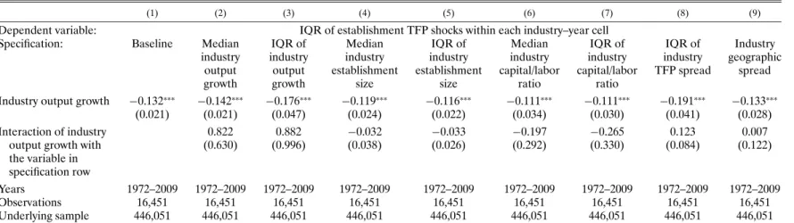
TableIIdisplays a series of industry panel regressions in which our dependent variable is the IQR of TFP shocks for all establishments in each industry (i)–year (t) cell. The regression specification that we run is
IQRit=ai+bt+γ yit
The explanatory variable in column (1) ( yit) is the median growth rate of output
1040
BLOOM
ET
AL.
TABLE II
UNCERTAINTY ISALSOROBUSTLYHIGHER AT THEINDUSTRYLEVELDURINGINDUSTRY“RECESSIONS”a
(1) (2) (3) (4) (5) (6) (7) (8) (9)
Dependent variable: IQR of establishment TFP shocks within each industry–year cell
Specification: Baseline Median IQR of Median IQR of Median IQR of IQR of Industry
industry industry industry industry industry industry industry geographic
output output establishment establishment capital/labor capital/labor TFP spread spread
growth growth size size ratio ratio
Industry output growth −0.132∗∗∗ −0.142∗∗∗ −0.176∗∗∗ −0.119∗∗∗ −0.116∗∗∗ −0.111∗∗∗ −0.111∗∗∗ −0.191∗∗∗ −0.133∗∗∗
(0.021) (0.021) (0.047) (0.024) (0.022) (0.034) (0.030) (0.041) (0.028)
Interaction of industry 0.822 0.882 −0.032 −0.033 −0.197 −0.265 0.123 0.007
output growth with (0.630) (0.996) (0.038) (0.026) (0.292) (0.330) (0.084) (0.122)
the variable in specification row
Years 1972–2009 1972–2009 1972–2009 1972–2009 1972–2009 1972–2009 1972–2009 1972–2009 1972–2009
Observations 16,451 16,451 16,451 16,451 16,451 16,451 16,451 16,451 16,451
Underlying sample 446,051 446,051 446,051 446,051 446,051 446,051 446,051 446,051 446,051
aEach column reports the results from an industry-by-year OLS panel regression, including a full set of industry and year fixed effects. The dependent variable in every column is the interquartile range (IQR) of establishment-level TFP shocks within each SIC four-digit industry–year cell. The regression sample is the 16,451 industry–year cells of the population of manufacturing establishments with 25 years or more of observations in the ASM or CM survey between 1972 and 2009 (which contains 446,051 underlying establishment years of data). These industry–year cells are weighted in the regression by the number of establishment observations within that cell, with the mean and median number of establishments per industry–year cell equal to 27.1 and 17, respectively. The TFP shock is calculated as the residual from the regression of log(TFP)at yeart+1on its lagged value (yeart), a full set of year dummies, and establishment fixed effects. In column 1, the explanatory variable is the median of the establishment-level output growth in that industry–year. In columns 2–9, a second variable is also included that is an interaction of that explanatory variable with an industry-level characteristic. In columns 2 and 3, this is the median and IQR of industry-level output growth, in columns 4 and 5 this is the median and IQR of industry-level establishment size in employees, in columns 6 and 7, this is the median and IQR of industry-level capital/labor ratios, in column 8 this is the IQR of industry-level TFP levels (note the mean is zero by construction), while finally in column 9, this interaction is the dispersion of industry-level concentration measured using the Ellison–Glaeser dispersion index. Standard errors clustered by industry are reported in brackets below every point estimate.∗∗∗denotes 1% significance,∗∗denotes 5% significance, and∗denotes 10% significance.
UNCERTAIN BUSINESS CYCLES 1041 fixed effects also included. Column 1 of TableIIshows that the within-industry dispersion of TFP shocks is significantly higher when that industry is growing more slowly. Since the regression has a full set of year and industry dummies, this is independent of the macroe-conomic cycle. So at both the aggregate and the industry level, slowdowns in growth are associated with increases in the cross-sectional dispersion of shocks.
This result raises the question of why the within-industry dispersion of shocks is higher during industry slowdowns. To explore whether it is the case that industry slowdowns impact some types of establishments differently, we proceed as follows. In columns 2–9, we run a series of regressions to check whether the increase in within-industry dispersion is larger given some particular characteristics of the industry. These are regressions of the form
IQRit=ai+bt+γ yit+δ yit∗xi
wherexiare industry characteristics (see Appendix A for details). Specifically, in column
2, we interact industry growth with the median growth rate in that industry over the full period. The rationale is that perhaps faster growing industries are more countercyclical in their dispersion? We find no relationship, suggesting long-run industry growth rates are not linked to the increase in dispersion of establishment shocks they see in recessions. Similarly, in column 3, we interact industry growth with the dispersion of industry growth rates. Perhaps industries with a wide spread of growth rates across establishments are more countercyclical in their dispersion? Again, we find no relationship. The rest of the table reports similar results for the median and dispersion of plant size within each indus-try (measured by the number of employees, columns 4 and 5), the median and dispersion of capital/labor ratios (columns 6 and 7), and TFP and geographical dispersion interac-tions (columns 8 and 9). In all of these we find insignificant coefficients on the interaction of industry growth with industry characteristics.
Thus, to summarize, it appears that, first, the within-industry dispersion of establish-ment TFP shocks rises sharply when the industry growth rates slow down, and, second, perhaps surprisingly, this relationship appears to be broadly robust across all industries.
An obvious question regarding the relationship between uncertainty and the business cycle is the direction of causality. Identifying the direction of causation is important in highlighting the extent to which countercyclical macro-uncertainty and industry uncer-tainty is a shock driving cycles versus an endogenous mechanism amplifying cycles. A re-cent literature has suggested a number of mechanisms for uncertainty to increase en-dogenously in recessions. See, for example, the papers on information collection byVan Nieuwerburgh and Veldkamp (2006), Fajgelbaum, Schaal, and Tascherau-Dumouchel (2017) or Chamley and Gale (1994), on experimentation in Bachmann and Moscarini (2011), on forecasting byOrlik and Veldkamp(2015), on policy uncertainty byLubos and Veronesi(2013), and on search byPetrosky-Nadeau and Wasmer(2013). Our view is that recessions appear to be initiated by a combination of negative first- and positive second-moment shocks, with ongoing amplification and propagation from uncertainty move-ments. So the direction of causality likely goes in both directions, and while we model the causal impact of uncertainty in this paper, more work on the reverse (amplification) direction would also be helpful.
2.3. Are Establishment-Level TFP Shocks a Good Proxy for Uncertainty?
The evidence we have provided for countercyclical aggregate and industry-level un-certainty relies heavily on using the dispersion of establishment-level TFP shocks as a
1042 BLOOM ET AL.
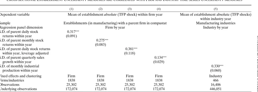
measure of uncertainty. To check this, TableIIIcompares our establishment TFP shock measure of uncertainty with other measures of uncertainty, primarily the volatility of daily and monthly firm-stock returns, which have been used commonly in the prior uncertainty literature.6Importantly, we note that the goal of this section is to demonstrate the
cor-relation between the different measures of uncertainty. Thus, this section does not imply any direction of causation.
In column 1 of Table III, we regress the mean absolute size of the TFP shock in the plants of publicly traded firms against their parent firm’s within-year volatility of daily stock returns (plus a full set of firm and year fixed effects). The positive and highly signif-icant coefficient reveals that when plants of publicly quoted firms have large (positive or negative) TFP shocks in any given year, their parent firms are likely to have significantly more volatile daily stock returns over the course of that year. This is reassuring for both our TFP shock measure of uncertainty and stock market volatility measures of uncer-tainty, because while neither measure is ideal, the fact that they are strongly correlated suggests that they are both proxies for an underlying measure of firm-level uncertainty. In column 2, we use monthly returns rather than daily returns and find similar results, while in column 3, followingLeahy and Whited(1996), we leverage adjust the stock returns and again find similar results.7
In column 4, we compare instead the within-year standard deviation of firm quarterly sales growth against the absolute size of their establishment TFP shocks. We find again a strikingly significant positive coefficient, showing that firms with a wider dispersion of TFP shocks across their plants tend to have more volatile sales growth within the year. Finally, in column 5, we generate an industry-level measure of output volatility within the year by taking the standard deviation of monthly production growth, and we find that this measure is also correlated with the average absolute size of establishment-level TFP shocks within the industry in that year.
So in summary, establishment-level TFP shocks are larger when the parent firms have more volatile stock returns and sales growth within the year, and the overall industry has more volatile monthly output growth within the year. This suggests that these indicators are all picking up some type of common movement in uncertainty.
2.4. Macroeconomic Measures of Uncertainty
The results discussed so far focus on establishing the countercyclicality of idiosyncratic (establishment, firm, and industry) uncertainty. With respect to macroeconomic uncer-tainty, existing work has documented that this measure is also countercyclical, including, for example,Schwert(1989), Campbell et al. (2001),Engle and Rangel(2008),Jurado, Ludvigson, and Ng(2014), andStock and Watson(2012), or the survey inBloom(2014).
Rather than repeat this evidence here, we simply include one additional empirical mea-sure of aggregate uncertainty, which is the conditional heteroskedasticity of aggregate productivity At. This is estimated using a generalized autoregressive conditional
het-eroskedasticity GARCH(11) estimator on theBasu, Fernald, and Kimball(2006) data
6See, for example,Leahy and Whited(1996),Schwert(1989),Bloom, Bond, and Van Reenen(2007), and Panousi and Papanikolaou(2012).
7As we did in column 7 of TableI, to remove the forecastable component of stock returns, we repeat columns 1 and 3, first removing the quarter by firm mean of firm returns. After doing this the coefficient (standard error) is very similar 0.324 (0.093) for column 1 and 0.387 (0.120) for column 3, mainly because the forecastable component of stock returns explains very little of the total volatility in stock returns.
UNCER T A IN BUSINESS CY CLES 1043 TABLE III
CROSS-SECTIONALESTABLISHMENTUNCERTAINTYMEASURES ARECORRELATEDWITHFIRM ANDINDUSTRYTIMESERIESUNCERTAINTYMEASURESa
(1) (2) (3) (4) (5)
Dependent variable Mean of establishmentabsolute(TFP shock) within firm year Mean of establishment absolute (TFP shocks) within industry year
Sample Establishments (in manufacturing) with a parent firm in compustat Manufacturing industries
Regression panel dimension Firm by year Industry by year
S.D. of parent daily stock 0.317∗∗∗
returns within year (0.091)
S.D. of parent monthly stock 0.275∗∗∗
returns within year (0.083)
S.D. of parent daily stock returns 0.381∗∗∗
within year, leverage adjusted (0.118)
S.D. of parent quarterly sales 0.134∗∗∗
growth within year (0.029)
S.D. of monthly industrial 0.330∗∗∗
production within year (0.060)
Fixed effects and clustering Firm Firm Firm Firm Industry
Firms/industries 1838 1838 1838 1838 466
Observations 25,302 25,302 25,302 25,302 16,406
Underlying observations 172,074 172,074 172,074 172,074 446,051
aThe dependent variable is the mean of the absolute size of the TFP shock at the firm–year level (columns 1–4) and industry–year level (column 5). This TFP shock is calculated as the residual from the regression of log(TFP)at yeart+1on its lagged value (yeart), a full set of year dummies, and establishment fixed effects, with the absolute size generated by turning all negative values positive. The regression sample in columns 1–4 are the 25,302 firm–year cells of the population of manufacturing establishments with 25 years or more of observations in the ASM or CM survey between 1972 and 2009 that are owned by Compustat (publicly listed) firms. This covers 172,074 underlying establishment years of data. The regression sample in column 5 is the 16,406 industry–year cells of the population of manufacturing establishments with 25 years or more of observations in the ASM or CM survey between 1972 and 2009. The explanatory variables in columns 1–3 are the annual standard deviation of the parent firm’s stock returns, which are calculated using the 260 daily values in columns 1 and 3 and the 12 monthly values in column 2. For comparability of monthly and daily values, the coefficients and S.E. for the daily returns in columns 1 and 3 are divided by sqrt(21). The daily stock returns in column 3 are normalized by the(equity/(debt+equity))ratio to control for leverage effects. In column 4, the explanatory variable is the standard deviation of the parent firm’s quarterly sales growth. Finally, in column 5, the explanatory variable is the standard deviation of the industry’s monthly industrial production data from the Federal Reserve Board. All columns have a full set of year fixed effects, with columns 1–4 also having firm fixed effects while column 5 has industry fixed effects. Standard errors clustered by firm/industry are reported in brackets below every point estimate.∗∗∗denotes 1% significance,∗∗denotes 5% significance, and∗denotes 10% significance.
1044 BLOOM ET AL.
on quarterly TFP growth from 1972Q1 to 2010Q4. We find that conditional heteroskedas-ticity of TFP growth is strongly countercyclical, rising by 25% during recessions, which is highly significant (at-statistic of 6.1); this series is plotted in Appendix Figure A2.
3. THE GENERAL EQUILIBRIUM MODEL
We proceed by analyzing the quantitative impact of variation in uncertainty within a DSGE model. Specifically, we consider an economy with heterogeneous firms that use capital and labor to produce a final good. Firms that adjust their capital stock and em-ployment incur adjustment costs. As is standard in the RBC literature, firms are subject to an exogenous process for productivity. We assume that the productivity process has an aggregate and an idiosyncratic component. In addition to the standard first-moment shocks considered in the literature, we allow the second moment of the innovations to productivity to vary over time. That is, shocks to productivity can be fairly small in normal times, but become potentially large when uncertainty is high.
3.1. Firms
3.1.1. Technology
The economy is populated by a large number of heterogeneous firms that employ cap-ital and labor to produce a single final good. We assume that each firm operates a dimin-ishing returns to scale production function with capital and labor as the variable inputs. Specifically, a firm indexed byjproduces output according to
yjt=Atzjtkαjtn ν
jt α+ν <1 (5)
Each firm’s productivity is a product of two separate processes: aggregate productivity, At, and an idiosyncratic component,zjt. Both the macro- and firm-level components of
productivity follow autoregressive processes as noted in equations (2) and (3). We allow the variance of innovations to the productivity processes, σA
t andσ
Z
t , to vary over time
according to a two-state Markov chain. 3.1.2. Adjustment Costs
There is a wide literature that estimates labor and capital adjustment costs (e.g., Hayashi(1982),Nickell(1986),Caballero and Engel(1993),Caballero and Engel(1999), Ramey and Shapiro (2001), Hall (2004), Cooper and Haltiwanger (2006), Merz and Yashiv(2007), andCooper, Haltiwanger, and Willis(2015)). In what follows, we incor-porate all types of adjustment costs that have been estimated in Bloom (2009) to be statistically significant at the 5% level. As is well known in the literature, it is the pres-ence of nonconvex adjustment costs that leads to a real options (wait-and-see effect) of uncertainty shocks.
Capital Law of Motion. A firm’s capital stock evolves according to the standard law of motion
kjt+1=(1−δk)kjt+ijt (6)
whereδkis the rate of capital depreciation andijtdenotes investment.
Capital adjustment costs are denoted by ACk, and they equal the sum of (i) a fixed
disruption costFKfor any investment/disinvestment and (ii) a partial irreversibility resale
UNCERTAIN BUSINESS CYCLES 1045 of its purchase price). Formally,
ACk=I|i|>0y(z A k n)FK+S|i|
I(i <0) (7)
Hours Law of Motion. The law of motion for hours worked is governed by
njt=(1−δn)njt−1+sjt (8)
wheresjtdenotes the net flows into hours worked andδndenotes the exogenous
destruc-tion rate of hours worked (due to factors such as retirement, illness, exogenous quits, etc.).
Labor adjustment costs are denoted by ACn in total, and they equal the sum of (i) a
fixed disruption costFLand (ii) a linear hiring/firing cost, which is expressed as a fraction
of the aggregate wage (Hw). Formally,
ACn=I|s|>0y(z A k n)FL
+ |s|Hw (9)
Note that these adjustment costs in labor imply thatnjt−1is a state variable for the firm.
3.1.3. The Firm’s Value Function
We denote byV (k n−1 z;A σA σZ µ)the value function of a firm. The seven state
variables are given by (i) a firm’s capital stock,k, (ii) a firm’s hours stock from the pre-vious period, n−1, (iii) the firm’s idiosyncratic productivity, z, (iv) aggregate
productiv-ity, A, (v) the current value of macro-uncertainty, σA
, (vi) the current value of micro-uncertainty, σZ, and (vii) the joint distribution of idiosyncratic productivity and
firm-level capital stocks and hours worked in the last period,µ, which is defined for the space S=R+×R+×R+.
Denoting by primes the value of next period variables, the dynamic problem of the firm consists of choosing investment and hours to maximize
Vk n−1 z;A σA σZ µ (10) =max in ⎧ ⎨ ⎩ y−wA σA σZ µn−i −ACkk n−1 z k′;A σA σZ µ −ACnk n−1 z n;A σA σZ µ +EmA σA σZ µ ;A′ σA′ σZ′ µ′Vk′ n z′;A′ σA′ σZ′ µ′ ⎫ ⎬ ⎭
given a law of motion for the joint distribution of idiosyncratic productivity, capital, and hours,
µ′
=ΓA σA σZ µ
(11) and the stochastic discount factor,m, which we discuss below in Section3.4. The term w(A σA σZ µ)denotes the wage rate in the economy;K(k n
−1 z;A σA σZ µ)and
Nd(k n
−1 z;A σA σZ µ)denote the policy rules associated with the firm’s choice of
capital for the next period and current demand for hours worked. 3.2. Households
The economy is populated by a large number of identical households that we normalize to a measure 1. Households choose paths of consumption, labor supply, and investment in firm shares to maximize lifetime utility. We use the measureψto denote the one-period
1046 BLOOM ET AL.
purchased shares in firms. The dynamic problem of the household is given by WA σA σZ µ= max {CNψ′} U(C N)+βEWA′ σA′ σZ′ µ′ (12) subject to the law of motion forµand a sequential budget constraint
C+ qk′ n z;A σA σZ µdψ′k′ n z ≤wA σA σZ µN+ ρk n−1 z;A σA σZ µ dµ(k n−1 z) (13)
Households receive labor income as well as the sum of dividends and the resale value of their investments priced at ρ(k n−1 z;A σA σZ µ). With these resources the
house-hold consumes and buys new shares at a priceq(k′ n z;A σA σZ µ)per share of the
different firms in the economy. We denote byC(ψ A σA σZ µ),Ns(ψ A σA σZ µ),
andΨ′(k′ n z;A σA σZ µ)the policy rules that determine current consumption, time
worked, and quantities of shares purchased in firms that begin the next period with a capital stockk′and who currently employnhours with idiosyncratic productivityz.
3.3. Recursive Competitive Equilibrium
A recursive competitive equilibrium in this economy is defined by a set of quantity functions{C Ns Ψ′ K Nd}, pricing functions{w q ρ m}, and lifetime utility and value
functions{W V}, whereV and{K Nd}are the value and policy functions, respectively,
that solve (10), whileW and{C Ns Ψ′}are, respectively, the value and policy functions
that solve (12). There is market clearing in asset markets µ′k′ n z′=
ψ′k′ n zfz′|zdz
the goods market Cψ A σA σZ µ = Azk αNdk n −1 z;A σA σZ µ ν −Kk n−1 z;A σA σZ µ −(1−δk)k −ACkk Kk n−1 z;A σA σZ µ −ACnn−1 N k n−1 z;A σA σZ µ dµ(k n−1 z)
and the labor market
Nsψ A σA σZ µ= Ndk n −1 z;A σA σZ µ dµ(k n−1 z)
Finally, the evolution of the joint distribution of z, k, and n−1 is consistent. That is,
Γ (A σA σZ µ)is generated byK(k n
−1 z;A σA σZ µ),Nd(k n−1 z;A σA σZ µ),
and the exogenous stochastic evolution ofA z σZ andσA, along with the appropriate
integration of firms’ optimal choices of capital and hours worked given current state vari-ables.
3.4. Sketch of the Numerical Solution
We briefly describe the solution algorithm, which heavily relies on the approach inKhan and Thomas(2008) andBachmann, Caballero, and Engel(2013). Fuller details are laid
UNCERTAIN BUSINESS CYCLES 1047 out in Appendix B, and the full code is available in the Supplementary Material (Bloom et al.(2018)).
The model can be simplified substantially if we combine the firm and the household problems into a single dynamic optimization problem. From the household problem, we get w= −UN(C N) UC(C N) (14) m=βUC C′ N′ UC(C N) (15)
where equation (14) is the standard optimality condition for labor supply and equation (15) is the standard expression for the stochastic discount factor. We assume that the momentary utility function for the household is separable across consumption and hours worked, U(Ct Nt)= C1−η t 1−η−θ Nχ t χ (16)
implying that the wage rate is given by
wt=θNtχ−1C η
t (17)
We define the intertemporal price of consumption goods asp(A σZ σA µ)≡U
C(C N).
This then allows us to redefine the firm’s problem in terms of marginal utility, denoting the new value function asV˜ ≡pV. The firm problem can then be expressed as
˜ Vk n−1 z;A σA σZ µ =max {in} pA σA σZ µy −wA σA σZ µn −i−ACk−ACn +βEV˜k′ n z′;A′ σA′ σZ′ µ′ (18) To solve this problem, we employ nonlinear techniques that build uponKrusell and Smith (1998). Detailed discussion of the algorithm is provided in Appendix B, where we imple-ment a range of alternative impleimple-mentations of our Krusell–Smith type algorithm. Impor-tantly, as we discuss in Appendix B, the main results remain robust across the different alternatives we consider.
4. PARAMETER VALUES
In this section, we describe the quantitative specification of our model. To maintain comparability with the RBC literature, we perform a standard calibration when possible (see Section4.1and TableIV). However, the parameters that govern the uncertainty pro-cess cannot be calibrated to match first moments in the U.S. data; neither have they been previously estimated in the literature. As such, we adopt a simulated method of moments (SMM) estimation procedure to choose these values in Section4.2. In Section5.2.3, we explore the sensitivity of the results to different parameter values.
1048
BLOOM
ET
AL.
TABLE IV
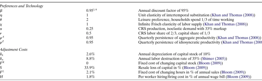
CALIBRATEDMODELPARAMETERSa Preferences and Technology
β 0951/4 Annual discount factor of 95%
η 1 Unit elasticity of intertemporal substitution (Khan and Thomas (2008))
θ 2 Leisure preference, households spend 1/3 of time working
χ 1 Infinite Frisch elasticity of labor supply (Khan and Thomas (2008))
α 025 CRS production, isoelastic demand with 33% markup
ν 05 CRS labor share of 2/3, capital share of 1/3
ρA 095 Quarterly persistence of aggregate productivity (Khan and Thomas (2008))
ρZ 095 Quarterly persistence of idiosyncratic productivity (Khan and Thomas (2008))
Adjustment Costs
δk 26% Annual depreciation of capital stock of 10%
δn 88% Annual labor destruction rate of 35% (Shimer (2005))
FK 0 Fixed cost of changing capital stock (Bloom (2009))
S 339% Resale loss of capital in % (Bloom (2009))
FL 21% Fixed cost of changing hours in % of annual sales (Bloom (2009))
H 18% Per worker hiring/firing cost in % of annual wage bill (Bloom (2009))
UNCERTAIN BUSINESS CYCLES 1049 4.1. Calibration
Frequency and Preferences
We set the time period to equal a quarter. The household’s discount rate, β, is set to match an annual interest rate of 5%. The variable η is set equal to 1, which im-plies that the momentary utility function features an elasticity of intertemporal substi-tution of 1 (i.e., log preferences in consumption). Following Khan and Thomas(2008) andBachmann, Caballero, and Engel(2013), we assume thatχ=1. This assumption im-plies that we do not need to forecast the wage rate in addition to the forecast ofpin our Krusell–Smith algorithm, since the household’s labor optimality condition withχ=1 im-plies that the wage is a function ofpalone. We set the parameterθsuch that households spend about a third of their time working in the nonstochastic steady state.
Production Function, Depreciation, and Adjustment Costs
We setδk to match a 10% annual capital depreciation rate. Based onShimer(2005),
we set the annual exogenous quit rate to 35%. We set the exponents on capital and labor in the firm’s production function to beα=025 andν=05, consistent with a capital cost share of 1/3 of total input costs.
As previously discussed, the existing literature provides a wide range of estimates for capital and labor adjustment costs. We use adjustment cost parameters from Bloom (2009). The resale loss of capital amounts to 34%. The fixed cost of adjusting hours is set to 21% of annual sales, and the hiring and firing costs equal 18% of annual wages.
Aggregate and Idiosyncratic TFP Processes
Productivity, both at the aggregate and the idiosyncratic level, is determined by AR(1) processes as specified in equations (2) and (3). The serial autocorrelation parametersρA
andρZ are set to 0.95, similar to the quarterly value used byKhan and Thomas(2008).
4.2. Estimation The Uncertainty Process
We assume that the stochastic volatility processes, σA
t and σ Z t , follow a two-point Markov chain: σA t ∈ σA L σ A H where PrσA t+1=σ A j |σ A t =σ A k =πσA kj (19) σZ t ∈ σZ L σ Z H where PrσZ t+1=σ Z j |σ Z t =σ Z k =πσZ kj (20)
Since we cannot directly observe the stochastic process of uncertainty in the data, we pro-ceed with SMM estimation. We formally discuss in Appendix C the estimation procedure and all relevant details.
Since the empirical results in Section2suggested that microeconomic and macroeco-nomic uncertainty co-move through the business cycle, we assume that a single process determines the economy’s uncertainty regime. That is, our assumption of a single uncer-tainty process implies that whenever microeconomic unceruncer-tainty is low (or high), so is macroeconomic uncertainty. This assumption reduces the number of parameters govern-ing the uncertainty process to six:σA
L,σ A H,σ Z L,σ Z H,π σ LH, andπ σ HL.
As the uncertainty process has a direct impact on observable cross-sectional and ag-gregate time-series moments, it is natural that the SMM estimator minimizes the sum of
1050 BLOOM ET AL. TABLE V
ESTIMATEDUNCERTAINTYPARAMETERSa Quantity Estimate Standard Error
σA
L 067 (0.098) Quarterly standard deviation of macroproductivity shocks (%)
σA
H/σLA 16 (0.015) Macrovolatility increase in high uncertainty state
σZ
L 51 (0.807) Quarterly standard deviation of microproductivity shocks (%)
σZ
H/σLZ 41 (0.043) Microvolatility increase in high uncertainty state
πσ
LH 26 (0.485) Quarterly transition probability from low to high uncertainty (%)
πσ
HH 943 (16.38) Quarterly probability of remaining in high uncertainty (%) aThe uncertainty process parameters are structurally estimated through an SMM procedure (see the main text and Appendix C in the Supplemental Material). The estimation process targets the time-series moments of the cross-sectional interquartile range of the establishment-level shock to estimated productivity in the Census of Manufactures and Annual Survey of Manufactures manufac-turing sample, along with the time-series moments of estimated heteroskedasticity of the U.S. aggregate Solow residual based on a GARCH(11)model. Both sets of target moments from the data are computed from 1972 to 2010.
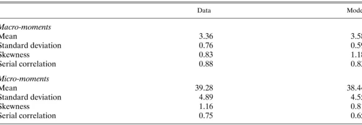
squared percentage deviations of the following eight model and U.S. data moments: At the microeconomic level, we target the (i) mean, (ii) standard deviation, (iii) skewness, and (iv) autocorrelation of the time series of the cross-sectional interquartile range of es-tablishment TFP shocks computed from our annual Census sample covering 1972–2010. At the macrolevel, we target the same four moments based on the time series of estimated heteroskedasticity using a GARCH(11)model for the annualized quarterly growth rate of the U.S. Solow residual, covering 1972Q1–2010Q4. We display the estimated uncer-tainty process parameters in TableVand the targeted moments in TableVI.
Based on this estimation procedure, we find that periods of high uncertainty occur with a quarterly probability of 26%. The period of heightened uncertainty is estimated to be persistent with a quarterly probability of 94% of staying in the high uncertainty state. Aggregate volatility is 067% with low uncertainty and increases by approximately 60% when an uncertainty shock arrives. Idiosyncratic volatility is estimated to equal 51% and
TABLE VI
UNCERTAINTYPROCESSMOMENTSa
Data Model Macro-moments Mean 336 358 Standard deviation 076 059 Skewness 083 118 Serial correlation 088 083 Micro-moments Mean 3928 3844 Standard deviation 489 455 Skewness 116 081 Serial correlation 075 065
aThe microdata moments are calculated from the U.S. Census of Manufactures and Annual Survey of Manufactures sample using annual data from 1972–2010. Microdata moments are computed from the cross-sectional interquartile range of the estimated shock to establishment-level productivity, in percentages. The model micro-moments are computed in the same fashion as the data moments, after correcting for measurement error in the data establishment-level regressions and aggregating to annual frequency. The macrodata moments refer to the estimated heteroskedasticity from 1972–2010 implied by a GARCH(11)model of the annualized quarterly change in the aggregate U.S. Solow residual, with quarterly data downloaded from John Fernald’s website. The model macro-moments are computed from an analogous GARCH(11)estimation on simulated aggregate data. All model results are based on a simulation of 1000 firms for 5000 quarters, discarding the first 500 periods.
UNCERTAIN BUSINESS CYCLES 1051 it increases by approximately 310% in the heightened uncertainty state. TableVreports the point estimates and standard errors from the SMM estimation procedure. As the table shows, most of these parameters are estimated precisely. However, in Section5.2.3, we discuss the robustness of our numerical results to modification of each of these six parameters.
It is useful at this point to explain the large estimated increase in underlying fundamen-tal microeconomic uncertaintyσZ
t on the impact of an uncertainty shock in light of the
apparently more muted fluctuations of our microeconomic uncertainty proxy in Figure3. Although closely related and informative for one another, the two series are distinct. Cru-cially, as we discuss in detail in our estimation Appendix C, the process of constructing our cross-sectional data proxy for microeconomic uncertainty involves time aggregation from quarterly to annual frequency, an unavoidable temporal mismatch of the measurement of inputs and outputs within the year, as well as measurement error of productivity in the underlying Census of Manufactures sample. In Appendix C, we demonstrate within the model that each of these measurement steps leads to a reduction in the variability of the uncertainty proxy relative to its mean level, with the temporal mismatch between input and output measurement, as well as measurement error itself, accounting for the bulk of the shift. The large increase in microeconomic uncertaintyσZ
t , which we estimate upon
impact of an uncertainty shock, is critical for matching the behavior of measured produc-tivity shock dispersion in the data. As TableVIdemonstrates, the estimated model quite closely captures the overall time-series properties of measured uncertainty in our data.
5. QUANTITATIVE ANALYSIS
In what follows, we explore the quantitative implications of our model. We begin by discussing the unconditional second moments generated by the model. We then continue by specifically studying the effects of an uncertainty shock.
5.1. Business Cycle Statistics
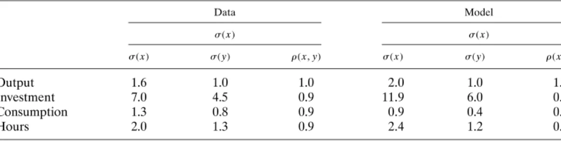
TableVIIillustrates that the model generates second-moment statistics that resemble their empirical counterparts in U.S. data. We simulate the model over 5000 quarters us-ing the histogram or nonstochastic simulation approach followus-ingYoung(2010). We then compute the standard set of business cycle statistics, after discarding an initial 500 quar-ters. As in the data, investment and hours co-move with output. Output and consumption co-move, although not as much as in the data. Investment is more volatile than output, while consumption is less volatile. Given the high assumed Frisch elasticity of labor sup-ply, the model also generates a realistic volatility of hours relative to output. SeeRogerson (1988),Hansen(1985), orBenhabib, Rogerson, and Wright(1991) for a discussion of un-derlying mechanisms that can generate more elastic labor supply in this class of models. Overall, we conclude that the business cycle implications of our model are consistent with the common findings in the literature.
5.2. The Effects of an Uncertainty Shock
As has been known since at leastScarf(1959), nonconvex adjustment costs lead toSs investment and hiring policy rules. Firms do not hire and invest until productivity reaches an upper threshold (theS inSs), and do not fire and disinvest until productivity hits a lower threshold (thesinSs). This is shown for labor in Figure5, which plots the distribu-tion of firms by their productivity/labor ratios, Az
1052 BLOOM ET AL. TABLE VII BUSINESSCYCLESTATISTICSa
Data Model σ(x) σ(x) σ(x) σ(y) ρ(x y) σ(x) σ(y) ρ(x y) Output 1.6 1.0 1.0 20 1.0 1.0 Investment 7.0 4.5 0.9 119 6.0 0.9 Consumption 1.3 0.8 0.9 09 0.4 0.5 Hours 2.0 1.3 0.9 24 1.2 0.8
aThe first panel contains business cycle statistics for quarterly U.S. data covering 1972Q1–2010Q4. The termσ(x)is the standard deviation of the log variable,σ(y)is the standard deviation in log variable relative to the standard deviation of log output, andρ(x y)
is the correlation of the log variable and log output. All business cycle data are current as of July 14, 2014. Output is real gross domestic product (FRED GDPC1), investment is real gross private domestic investment (GPDIC1), consumption is real personal consumption expenditures (PCECC96), and hours is total nonfarm business sector hours (HOANBS). The second panel contains business cycle statistics from unconditional simulation of the estimated model, computed from a 5000-quarter simulation with the first 500 periods discarded. All series are HP-filtered with smoothing parameter 1600, in logs expressed as percentages.
been drawn but before firms have adjusted. On the right is the firm-level hiring threshold (right solid line) and on the left the firing threshold (left solid line), in the case of low uncertainty. Firms to the right of the hiring line will hire, firms to the left of the firing line will fire, and those in the middle will be inactive for the period.
An increase in uncertainty increases the returns to inaction, shown by the increased hiring threshold (right dotted line) and reduced firing threshold (left dotted line). When uncertainty is high, firms become more cautious as labor adjustment costs make it
expen-FIGURE5.—The impact of an increase in uncertainty on the hiring and firing thresholds. Notes: The figure plots the simulated cross-sectional marginal distribution of micro-level labor inputs after productivity shock realizations and before labor adjustment. The distribution plots a representative period with average aggregate productivity and low uncertainty levels. The vertical hiring and firing thresholds are computed based on firm policy functions with average micro-level productivity realizations, taking as given the aggregate state of the economy with low uncertainty (solid lines) and a high uncertainty counterfactual (dotted lines).
UNCERTAIN BUSINESS CYCLES 1053 sive to make a hiring or firing mistake. Hence, the hiring and firing thresholds move out, increasing the range of inaction. This leads to a fall in net hiring, since the mass of firms is right-shifted due to labor attrition. A similar phenomenon occurs with capital, whereby increases in uncertainty reduce the amount of net investment.
5.2.1. Modelling a Pure Uncertainty Shock
To analyze the aggregate impact of uncertainty, we independently simulate 2500 economies, each of 100-quarter length. The first 50 periods are simulated unconditionally, so all exogenous processes evolve normally. Then for each economy, after 50 quarters, we insert an uncertainty shock by imposing a high uncertainty state. From the shock period onward each economy evolves normally. To calculate the impulse response function to an uncertainty shock for any macrovariable, we first compute the average of the aggregate variable in each periodtacross simulated economies. The effect of an uncertainty shock is then simply given by the percentage deviation of the average in periodtfrom its value in the pre-shock period.
Figure6depicts the impact of an uncertainty shock on output. For graphical purposes, period 0 in the figure corresponds to the pre-shock period in the above discussion, that is, quarter 50. Figure6displays a drop in output of just over 2.5% within one quarter. This significant fall is one of the key results of this paper as it shows that uncertainty shocks can be a quantitatively important contributor to business cycles within a general equilibrium framework. A quick recovery follows the initial decline, and output returns to normal levels within 1 year. We note that output then declines again moderately from quarters 6 onward. We defer the discussion for the intuition behind this result until Section5.2.4.
These dynamics in output arise from the dynamics in three channels: labor, capital, and the misallocation of factors of production. These are depicted in Figure7. First, in
FIGURE 6.—The effects of an uncertainty shock. Notes: Based on independent simulations of 2500 economies of 100-quarter length. We impose an uncertainty shock in the quarter labelled 1, allowing normal evolution of the economy afterwards. We plot the percent deviation of cross-economy average output from its value in quarter 0.