Multivariate Volatility Modelling for Cryptocurrencies

(1)

Faculty of Mathematics, Computer Science and Statistics

Chair of Financial Econometrics

Multivariate Volatility Modelling

for Cryptocurrencies

Master Thesis

Stephanie Riedl

Full Professor: Prof. Stefan Mittnik, PhD Supervisor: Malte Kurz, M. Sc.

(2)

I would like to acknowledge everyone who supported me during the creation of my thesis.

I first would like to thank my thesis advisor Malte Kurz. His door was always open for me to come with any problems or questions, and he always guided me in the right direction. His advice was on point and extremely helpful at any time, while he still allowed this thesis to be my own work.

Next, I want to thank Prof. Dr. Stefan Mittnik for his enthusiasm and input on the topic of this thesis.

I would also like to acknowledge Fernando Cuervo and my mother Christiane Riedl as second readers of this thesis, and I am grateful for their valuable comment. Finally, I would like to thank my family and friends who provided my with continu-ous support and encouragement throughout my whole academic career. They never failed to believe in me, even in times when I doubted myself. This accomplishment would not have been possible without them.

(3)

Cryptocurrencies as an investment have received increasing attention by media and international governments over the last years. However, little is known yet about the dynamics that drive these highly volatile alternative assets. This thesis studies the dynamic interdependencies between the volatility of Bitcoin, Litecoin, Ripple, Dogecoin and Feathercoin via the Dynamic Conditional Correlation model by Engle (2002) with the multivariate Student-t distribution. The main question is whether a multivariate approach improves the Value at Risk forecasting accuracy for the conditional heteroscedasticity in comparison to univariate GARCH-type models. Results show that there is a high interconnectedness between the volatility of the currencies. However, the Dynamic Conditional Correlation model can not deliver better forecasting results than the univariate GARCH-type models for the individ-ual cryptocurrency return series.

(4)

List of Figures iv

List of Tables v

1 Introduction 1

2 Background on Cryptocurrencies 4

3 Previous Research on Volatility of Cryptocurrencies 7

4 Univariate Volatility Modelling 10

4.1 Structure of Univariate Volatility Models . . . 10

4.2 Estimation . . . 15

4.3 Diagnostic Checking . . . 17

4.4 Value at Risk . . . 17

5 Univariate Empirical Results 20 6 Multivariate Volatility Modelling 40 6.1 Multivariate Conditional Heteroscedasticity . . . 40

6.2 Dynamic Conditional Correlation Models . . . 41

6.3 Estimation . . . 43

6.4 Diagnostic Checking . . . 44

7 Multivariate Empirical Results 46

8 Conclusion 58

References 65

A Appendix 66

B Electronic Attachments 69

(5)

1 The evolution of daily closing prices in $US for Bitcoin, Litecoin, Dogecoin, Ripple and Feathercoin from 17th _{of December 2013 until} 14th _{of March 2018. . . .} ₂₀ 2 Histograms of the log returns of the five cryptocurrencies and the

aggregated portfolio in blue. Log returns are calculated using: rt = 100×ln(Pt/Pt−1). Black line shows the density of the Normal dis-tribution that would occur for the empirical mean and standard de-viation: x∼N(ri,

p

V ar(ri)). T=1544. . . 24 3 The evolution of log returns in $US of Bitcoin, Litecoin, Dogecoin,

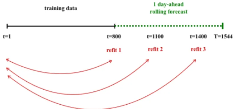
Ripple, Feathercoin and the aggregated portfolio until 14th _{of March} 2018. . . 25 4 Outline for the 1-day-ahead forecast. The time line shows the

train-ing data set of length T=800 in black and the rolltrain-ing out-of-sample forecast of length T=744 in green. Red arrows indicate the observa-tions included in the three parameter re-estimaobserva-tions (recursive win-dow). . . 29 5 Value at Risk forecasts for the 1-day-ahead rolling forecast of the 1/k

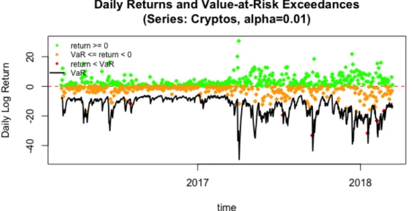
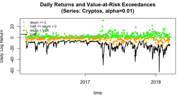
portfolio estimated with a univariate eGARCH with skewed Student-t disStudent-tribuStudent-tion. The model is built on a training data set of 800 observations, which leaves 744 out-of-sample forecasts. Parameters are re-estimated every 300 days with a recursive window, which leads to a total number of 3 refits. . . 35 6 Value at Risk forecasts for the 1-day-ahead rolling forecast of the 1/k

portfolio estimated with a univariate eGARCH with skewed Student-t disStudent-tribuStudent-tion. The model is built on a training data set of 800 observations, which leaves 744 out-of-sample forecasts. Parameters are re-estimated every10 dayswith a recursive window, which leads to a total number of 75 refits. . . 37 7 Model parameters for the rolling forecast of the aggregated portfolio.

eGARCH fit coefficients with robust standard error bands across 75 refits. Parameters are re-estimated every 10 days with a recursive window on a 744 day out-of-sample rolling 1-day-ahead forecast. . . 38 9 The estimated dynamic correlation between the currencies modelled

(6)

tion (57). The model is built on a training data set of 800 obser-vations, which leaves 744 out-of-sample forecasts. Parameters are re-estimated every 300 days with a recursive window, which leads to a total number of 3 refits. . . 54 11 Value at Risk forecasts for the 1-day-ahead rolling forecast of the

1/k portfolio estimated with a multivariate DCC according to equa-tion (57). The model is built on a training data set of 800 obser-vations, which leaves 744 out-of-sample forecasts. Parameters are re-estimated every 10 dayswith a recursive window, which leads to a total number of 75 refits. . . 55 12 Plot for the autocorrelation and partial autocorrelation of the squared

logarithmic returns of the individual cryptocurrency return series. Blue dashed line indicates the 5% significance level. . . 66 13 Quantile-to-quantile plots for the distribution of standardized errors

for the selected univariate GARCH models . . . 67 14 Autocorrelation of squared standardized errors for the selected

uni-variate GARCH models. Red dashed line indicates the 5% signifi-cance level. . . 68

(7)

1 Summary Statistics for daily log returns × 100 of cryptocurrencies. Log returns are calculated using: rt= 100×ln(Pt/Pt−1). Returns are observed until 14th _{of March 2018. Market cap is captured at 14}th _of March 2018. Jarque-Bera-Test checks for deviation from normality (skewness S different from zero and kurtosis K different from 3): J B = T(S/6 + (k−3)2/24), is distributed as X2_{(2) with 2 degrees} of freedom. Its critical value at the five-percent level is 5.99 and at the one-percent it is 9.21. . . 21 2 AIC and BIC for the estimated GARCH-type models. µtis modelled

via an ARMA-(1,1) process. σt is modelled via a GARCH-type pro-cess of order (1,1). T=1544. Lowest AICs and BICs per group are written in bold letters. . . 27 3 1%- and 5%-Value at Risk results for the univariate GARCH-type

models. 1-day-ahead rolling forecast with recursive window, model parameters refitted every 300 observations. Model is built on a train-ing data set of 800 observations, which leaves 744 out-of-sample fore-casts. % Viol: Percentage of VaR violations at α= 1% andα = 5%. Luc: p-value for test of unconditional coverage; Lcc: p-value for test of conditional coverage. Values printed bold if p <0.05. . . 31 4 Model parameters of the selected GARCH models. µt is modelled

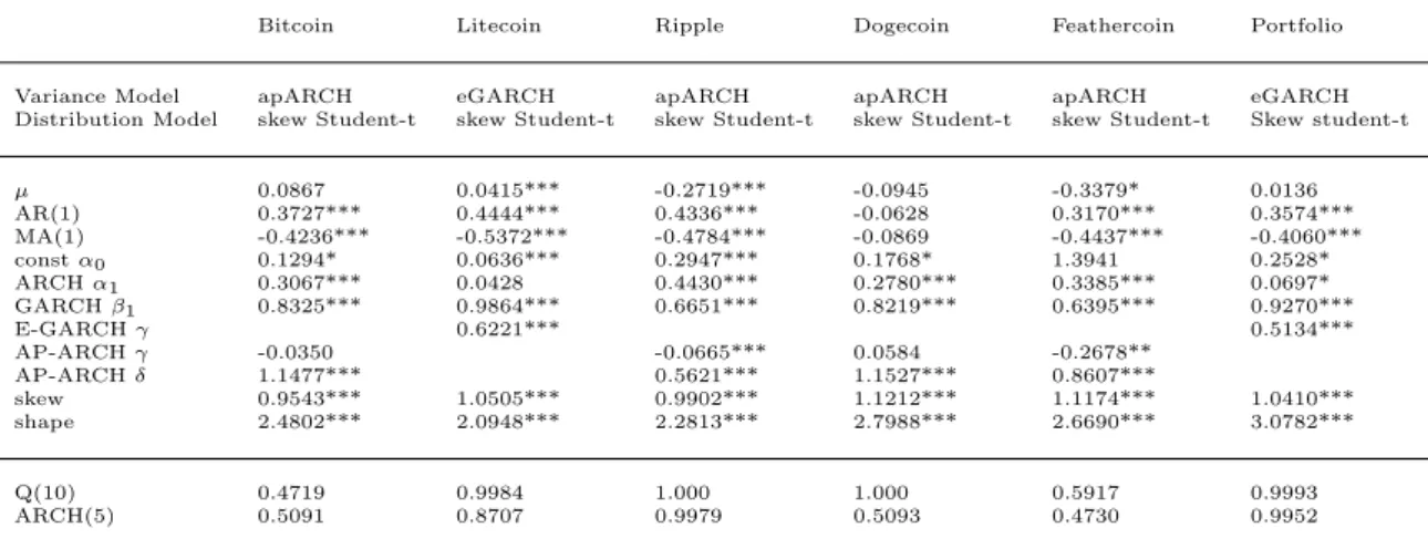
via an ARMA-(1,1) process. T=1544. *** p-value < 0.001; ** p-value <0.01; * p-value < 0.05. Q(10): p-value of Ljung-Box test on squared standardized residuals for lag ` = 10; ARCH(5): p-value for weighted ARCH LM test for lag `= 5. . . 34 5 Lag ` = 0 sample correlation matrix ˆρ0 (Pearson) of the five crypto

currency log return series. T = 1554. . . 46 6 Model parameters for the estimated DCC models. T=1544, k=5,

*** p-value < 0.001; ** p-value < 0.01; * p-value < 0.05. Model parameters for univariate volatility series are listed in table (4). . . 48 7 Mean and (standard deviation) of the lag ` = 0 correlations in the

multivariate volatility of the currencies estimated by the DCC model in equation (57). T=1544. . . 51

(8)

1 Introduction

Over the last years, the public interest in cryptocurrencies has increased dramati-cally. The decentralized peer-to-peer system makes cryptocurrencies an attractive phenomenon on the internet and many enthusiasts see it as an independent alterna-tive towards the traditional financial market which has experienced bad reputation ever since the market turmoil of 2008. Since mid 2017, many cryptocurrencies have experienced an extreme price increase which provided the early adopters with an immense return for their former low priced investments. The cryptocurrency market has been extremely volatile since then, which has lead to a lot of economic and sci-entific attempts to understand and predict the risk of investment. Previous analyses have focused on the determinants of cryptocurrency prices or their interconnected-ness with traditional markets. Other authors studied the sociodemographic profile of cryptocurrency buyers and tried to find relations with social media and browsing activities. Yelowitz and Wilson (2015) analysed Google trends data and found that a high interest in Bitcoin is positively correlated with computer programming and illegal activity search terms online.

Many academic analyses focus on understanding the highly volatile behaviour of the price developments. Using GARCH-type models to determine the risk of Bitcoin and other cryptocurrencies has become a popular topic in academic research over the last two years. However, less is known yet about the interdependencies between the volatility behaviour of different coins.

The main attempt of this thesis is to explore whether a multivariate approach can improve the modelling and forecasting of volatility for the selected cryptocurrencies. It is to find out if there are any correlations and mutual dynamics in the altcoin market that help to determine the volatility of the single currencies or if the trends are very particular for every currency and they are modelled more appropriately via a univariate approach. Therefore, there are GARCH-type models applied to the univariate log return series first. Several variance models from the GARCH family are utilized to model the evolution of the conditional variance of the return series. For the distribution of the innovations, heavy-tailed and skewed alternatives are applied next to the Gaussian distribution since previous research has brought up findings in favour of heavy-tailed distributions for the returns of financial as-sets. The different models with different distribution assumptions are going to be evaluated via model diagnostics and information criteria, as well as their ability to forecast the downside portfolio risk (VaR). Next to the single return series of the

(9)

five analysed currencies, an aggregated portfolio is also modelled via a univariate approach.

The results of the univariate empirical analysis are going to be used to proceed to a multivariate volatility modelling approach. The residuals of the selected GARCH models are implemented to model the time-varying covariance of the volatility of the five currencies. The multivariate Dynamic Conditional Correlation model by Engle (2002) thus is applied to the multivariate log return series. The fit of the multivariate Normal distribution for the innovations is outperformed by the multi-variate Student-t distribution. After fitting the DCC model, its ability to forecast Value at Risk for an aggregated portfolio is evaluated and eventually compared to the results for the univariate GARCH models.

The thesis is organized as follows: First, there is an introduction on the cryptocur-rencies used in this paper. The curcryptocur-rencies Bitcoin (BTC), Litecoin (LTC), Ripple (XRP), Dogecoin (DOGE) and Feathercoin (FTC) are selected because they have been operational for some time already, which is in favour of statistical time series analysis. There is a short description of the single currencies, pointing out the main technical differences between them. This is followed by a review of previous litera-ture on volatility modelling for cryptocurrencies. The majority of authors focus on GARCH-type models for Bitcoin - the most popular currency on the altcoin market. The choice for a certain GARCH model differs, but most authors have found the Gaussian distribution to be inappropriate to model the innovations of the log re-turn series and proceed to skewed alternatives. Other authors analyse the dynamics between cryptocurrencies and the traditional asset market. Fewer have focussed on the multivariate dynamics between the volatility of different crypto coins so far.

It follows a theoretical section with an explanation of the model equations of the different applied GARCH type models. Also there is an overview of the different dis-tributions that the innovations are assumed to follow. Besides the Normal distribu-tion, the heavy-tailed Student-t distribudistribu-tion, as well as its skewed modification and the skewed Generalized Error distribution are described. The Maximum-Likelihood estimation for the simple GARCH model by Bollerslev (1986) is outlined. Then, there is an explanation of the different model diagnostics that are appropriate for financial volatility analysis. Since the models are also evaluated by their ability to forecast the realized portfolio loss, the riskmetric Value at Risk and its application to GARCH processes is introduced.

(10)

se-and heavy-tailed distribution of the log returns that is typical for financial time series. Also, an analysis of the autocorrelation of the returns reveals conditional heteroscedasticity in the data, which justifies the application of GARCH models. The different GARCH models, namely the simple GARCH, eGARCH, iGARCH, apARCH, cs-GARCH and gjr-GARCH with the different distribution assumptions for the innovations are applied to the series and compared via diagnostic checking, information criteria and Value at Risk forecasts. The results show that the Gaussian distribution is clearly outperformed by the heavy-tailed distributions when it comes to model fit and forecasting performance. The apARCH, eGARCH and csGARCH, combined with the skewed Student-t or skewed Generalized error distribution for the innovations, seem to be most appropriate to model and forecast the dynamics of the univariate volatility. Then, the out-of-sample rolling forecast is executed with a higher number of model refits for the aggregated portfolio. It shows that a more frequent update of model parameters does not improve the forecasting results. The next section outlines the theoretical framework for the multivariate analysis. Since the estimation of Dynamic Conditional Correlation models requires higher computational effort, the presence of multivariate conditional heteroscedasticity in the data should be detected ex ante. Therefore, it is useful to apply the multivariate Ljung-Box test to find time-variant dependencies in the cross correlation matrix. Then, the Dynamic Conditional Correlation model by Engle (2002) is defined. The model estimates the dynamic correlation matrix of the standardized innovations from the univariate series and thus models dynamics between the data. The condi-tional distribution of the multivariate volatility can be modelled by a multivariate Gaussian distribution or the multivariate Student-t distribution. Next, the 2-stage estimation of the DCC via Quasi-Maximum-Likelihood is described. At the first stage, the volatility of the univariate return series is obtained and the standard-ized residuals are used to estimate the mutual conditional correlation matrix at the second stage. The last chapter for the theoretical framework gives an overview of additional model diagnostic techniques that can be applied to the multivariate residuals.

After that, the results for the multivariate part of the empirical analysis are pre-sented. Multivariate conditional heteroscedasticity in the sample correlation ma-trix is detected, which justifies the application of the DCC. Several DCC orders are applied with the conditional multivariate Normal and multivariate Student-t distribution, using the results from the univariate GARCH analysis to estimate the correlation of volatilities. It shows that a simple DCC order of lags (1,1) with the multivariate Student-t distribution provides the most appropriate fit according to

(11)

information criteria. After fitting the model, a rolling out-of-sample forecast for the Value at Risk is performed. Therefore, an aggregated portfolio is created. Its dis-tribution is determined by the forecasted mean and covariance matrix of the DCC, according to the approach by Bauwens and Laurent (2005). However, the Value at Risk forecast with the multivariate approach does not show more accurate results than the univariate approach for the aggregated portfolio. Moreover, Value at Risk forecasting of the univariate individual return series can not be outperformed by the aggregated univariate or multivariate approach.

As a final conclusion, the results and their limitations are discussed and implications for further research are given.

2 Background on Cryptocurrencies

A cryptocurrency can be defined as ”a digital asset designed to work as a medium of exchange using cryptography to secure the transactions and to control the creation of additional units of the currency” (Chu et al., 2017, pg. 1).

In the following section, there is a brief overview on the five cryptocurrencies that are used in this study. Cryptocurrencies are digital currencies and mainly characterized by their decentralization and trading on an online peer-to-peer network. The digital coins are generated via cryptographic techniques and recorded and verified by the community. Bitcoin was the first decentralized currency emerging in 2008 and has entailed many successors. The website Coinmarketcap.com lists 1969 different operating cryptocurrencies in September 2018. The five currencies used in this thesis were chosen since they are operational for a long time and provide a high observation span, which is of benefit to statistical analysis.

Bitcoin (BTC) is the first cryptocurrency and has been operational since 2009. In 2008, a person with the pseudonym ”Natoshi Sakomoto” created a document on the alternative currency, which has become the most traded coin on the market to-day. It was the first decentralized currency that runs on a peer-to-peer network with transactions between users happening without mediation by a third party (e.g. a financial institution). The transactions are recorded via aBlockchain, an extendible list of datasets that are connected by cryptographic procedures and verified by a network of individuals using the Bitcoin software. The individuals who offer their computer power to keep track of the transactions are called miners. Miners solve

(12)

created, which gives further incentive to miners on top of transaction fees (Chuen et al., 2017). When Sakomoto first published his document on the new cryptocur-rency, there were still 50 BTC generated during the mining process of one block. The supply of Bitcoin is limited to 21 million and the reward drops by 50% after every 210.000 transaction blocks (Nakamoto, 2008). In September 2018, the reward for every mined block is 12.5 coins and only 18 percent of the Bitcoins are left to be mined (Blockchainhalf.com).

Due to the immense consumption of computation power - a regular PC would need several years to solve a puzzle - mining has become non profitable for individuals and mainly been commercialized over the last years (Chuen et al., 2017).

The usage of cryptographic techniques ensures that transactions of Bitcoins can only be executed by the Bitcoin owners and the currency can not be spent twice. The system is safe against transaction hackers since changing the transaction his-tory would require redoing all puzzles of all blocks linked together in the chain. That again would take enormous computational power for the hacker (Nakamoto, 2008).

The source code for Bitcoin is publicly available online on Github.com, which has motivated many successors to create alternative cryptocurrencies with improved qualities.

Litecoin (LTC) released in October 2011, is one of the most important successors of Bitcoin and its operation is nearly identical to Bitcoin. It is a peer-to-peer decen-tralized currency based on an open source security protocol, published in October 2011 by Charles Lee (Chuen et al., 2017). The only difference to Bitcoin is that blocks are generated faster (2,5 minutes instead of 10), which is why transactions by users can be made faster. Therefore, higher trading volumes can be handled and the network is scheduled to produce 84 million coins eventually (Litecoin.org). Ripple (XRP) was developed completely independent from Bitcoin. It is built on an open source decentralized consensus protocol, even though the deployment is provided by Ripple Labs who hold 25% of the currency, next to 20% held by the founders. It is operating since 2012. In general, Ripple is based on a public data bank where different account balances are registered. Additionally, the register contains options on goods and traditional currencies (Dollar, Yen, etc.) which can be bought in the system using the intern currency ”XRP”. XRP can either be traded itself or used to make payments for other goods and currencies.

(13)

the trading in the system, and validating servers that run the protocol in the system to check and validate transactions. All historic transactions and account balances are publicly available.

Just like Bitcoin, the transactions in the Ripple system are ensured by an Elliptic Curve Digital Signature Algorithm. But instead of using miners, Ripple relies on the consensus of the validating servers to vote for the correct transaction in the system. While Bitcoin transactions can only be confirmed after mining the blocks, which takes an hour on average, the consensus in Ripple system is reached within a few seconds. Therefore, faster payments are supported (Armknecht et al., 2015). Dogecoin (DOGE) was usually intended as a parody of Bitcoin and is named after the Shiba Inu dog ”Doge” which became a popular internet phenomenon in 2013. Dogecoin is based on the same operating system as Bitcoin and Litecoin, but the block generating algorithms work even faster than for Litecoin with one block being produced every minute. The ultimate number of Dogecoins is not limited (Dogecoin.com). The currency, which was originally intended as a joke, has experienced immense popularity after its creation in 2013. The trading of DOGE is processed in social networks like Reddit and Twitter (Chuen et al., 2017). Feathercoin (FTC) is another cryptocurrency which is based on the Bitcoin op-erating system and was released in April 2013. Just like other Bitcoin successors it works with a faster average block time of one minute. The total number of Feather-coins is limited to 336 millions, with a block reward halving every 2.1 million blocks. A special feature of Feathercoin is the Neoscript Algorithm that is used for mining and requires less computer power than the Bitcoin algorithms (Feathercoin.com). Therefore, Feathercoin experienced a hype in late 2013/early 2014 - see figure (1) in section (5) - but was eventually outperformed by other emerging currencies.

(14)

3 Previous Research on Volatility of

Cryptocur-rencies

The interest in the analysis of the variation in cryptocurrency prices mainly arises since they are highly volatile compared to traditional currencies. When invested at the right time, they provided their owners with immense profits. In the past two years, researchers have made effort to study the variations of cryptocurrency returns via Generalized Autoregressive Conditional Heteroscedasticity (GARCH) models. However, fewer studies have made effort to study the multivariate dynamics of the crypto market.

Most studies so far focus on the modelling of Bitcoin only, which is the first and most popular cryptocurrency. Its high market volume and long observation span makes it most attractive for statistical analysis. Since Bitcoin and other cryptocur-rencies have experienced immense popularity over the last years, a lot of academic effort has been made to determine the development of prices. A lot of studies have focused on the interconnectedness between Bitcoin and Twitter or Google activities. Georgoula et al. (2015) have shown that the Twitter sentiment ratio is positively related with Bitcoin prices. Other authors like Ciaian et al. (2016) have focused on the impact of investors and macro-economics and found that market forces and Bitcoin attractiveness for investors have a big influence on the short run but does not seem to influence the overall long-term price development.

Concerning stylized facts, cryptocurrency time series are characterized similarly to other financial time series. They exhibit time-varying volatility, extreme observa-tions and an asymmetry of the volatility process to the sign of past innovation (Catania et al., 2018). Just like other econometric time series, the log returns of the cryptocurrencies have been found to show major deviations from normality. Chu et al. (2017) find that seven of the most important currencies are positively skewed. They also show extreme volatility compared to traditional assets, espe-cially with regard to inter-daily prices. Gkillas and Katsiampa (2018) study the heavy-tail behaviour of Bitcoin, Bitcoin Cash, Etherum, Ripple and Litecoin. They find that cryptocurrencies are more risky and volatile than traditional currencies and also show heavier tail behaviour. Bitcoin and Litecoin showed to be the least risky currencies of the five analysed coins. Phillip et al. (2018) study the stylized facts of 224 different cryptocurrencies and find that they show leverage effects and a negative correlation between one-day ahead volatility and returns. They also find that the returns follow a Student-t distribution rather than a Normal distribution. Besides stylized facts, many authors have studied the conditional variance of the

(15)

individual cryptocurrency return series via Generalized Autoregressive Conditional Heteroscedasticity (GARCH) models. Chen et al. (2016) give one of the first anal-ysis of the dynamics in the CRIXindex family. The CRIX (CRypto currency In-deX) provides market information based on the 30 most important currencies and is modelled by a ARIMA(2,0,2)-t-GARCH(1,1) process to capture the volatility of the index return series. Chu et al. (2017) apply different univariate GARCH-type mod-els to seven of the most popular currencies (Bitcoin, Dash, Litecoin, MaidSafeCoin, Monero, Dogecoin and Ripple) and mainly claim the iGARCH and gjrGARCH to be the best models to explain univariate volatility for those currencies. They also show that cryptocurrencies exhibit extremely high volatility when they look at inter-daily prices.

Katsiampa (2017) explores several conditional heteroscedasticity models to Bitcoin and finds the autoregressive compenent GARCH model to fit the data best, which has both a long-run and a short-run component of conditional variance. Katsampias study has been replicated by Charles and Darn´e (2018) who use robust QML es-timators to fit the GARCH-type models instead of standard Maximum-Likelihood estimators to take the conditional non-normality of the returns into account. Im-provements in the estimation method again result in the choice of an AR-csGARCH process to describe the conditional heteroscedasticity in the Bitcoin return series. However, both papers miss out to investigate whether an alternative distribution like the Student-t or skewed Student-t distribution might fit the log returns better. Several studies have found that fat-tailed, possibly skewed distributions are more adequate to describe financial data (Kuester et al., 2006).

Angelini and Emili (2018) attempt to forecast the volatility for six cryptocurrencies with GARCH-type models. They compare the forecasting performance of the simple GARCH, eGARCH, tGARCH, GARCH-M and apARCH with a training dataset of 700 daily prices, combined with a Student-t distribution for the innovations. Then, they performh= 1, ...,7 steps-ahead forecasts with a recursive window. The eGARCH seems to perform best for the higher forecast horizons overall, however, results differ between the different currencies and forecasting horizons.

Catania and Grassi (2017) claim that standard volatility models like the GARCH are outperformed by alternatives like the Score Driven model with conditional Gen-eralized Hyperbolic Skew Student-t innovations (GHSKT). With the chosen model they legitimately react to the skewness of the distribution of the log returns, how-ever, they miss out on comparing the models via Value at Risk - performance is evaluated by AIC and BIC.

(16)

US stock market. Conrad et al. (2018) use the GARCH-MIDAS model to extract long-term and short-term volatility components of the Bitcoin price series. They find that the S&P realized volatility has a negative and highly significant effect on long-term Bitcoin volatility. According to their results, Bitcoin volatility is nega-tively correlated to the US stock market volatility.

However, fewer literature has focussed on the dynamic correlation of volatility be-tween the different cryptocurrencies yet, with the most papers on this issues being published in 2018. Corbet et al. (2018) study the relationship between Bitcoin, Ripple and Litecoin and other traditional financial indices by generalized variance decomposition methods and find that the price developments of cryptocurrencies are highly connected to each other while they are disconnected to mainstream assets on the long run. Spillovers between Bitcoin and traditional indices (e.g. SP500 and VIX) can only be observed on the short run.

Katsiampa (2018) employs an Asymmetric Diagonal BEKK multivariate GARCH model with a multivariate Student-t distribution for the error terms to the log re-turns of Bitcoin, Etherum, Ripple, Litecoin and Stellar to estimate the dynamic volatility of those currencies. He found that the conditional covariances were sig-nificantly affected by the past covariances of the innovations. The conditional cor-relation between the five currencies has shown to be mainly positive but changing over time.

The analysis of the evolution of different cryptocurrency volatilities has been a popular field of econometric research for the last two years. Many authors have already compared several univariate GARCH-type models to predict Value at Risk forecasts for the most popular cryptocurrencies and few focused on the dynamic in-terdependencies of conditional covariances. This thesis attempts to combine those two approaches and find out whether the performance of Value at Risk forecasting can be improved by employing a multivariate approach.

(17)

4 Univariate Volatility Modelling

This section deals with the theoretical framework for univariate volatility modelling and Value at Risk forecasting.

Volatility models are also referred to conditional heteroscedasticity models. Here, volatility means ”the conditional standard deviation of the underlying asset return” (Tsay, 2005, pg. 109). Volatility modelling provides a simple approach to calculat-ing Value at Risk of a financial position in risk management. It can improve the efficiency in parameter estimation and the accuracy in interval forecasting. Volatil-ity is not directly observable, however, it has some characteristics that are common for asset return series. First, there are volatility clusters - volatility may be high for certain periods and low for others. Second, volatility evolves over time in a continuous manner. Third, volatility does not diverge to infinity, but varies within some fixed range. Fourth, volatility seems to react differently to a big price increase or a big price drop, which is referred to as ”leverage effect”. (Tsay, 2005).

4.1 Structure of Univariate Volatility Models

Letrtbe the log return of an asset at time indext. In volatility modelling the series rt is serially uncorrelated but dependent. The conditional mean and variance of rt givenFt−1 can be described as

µt =E(rt|Ft−1), σt2 =V ar(rt|Ft−1) =E[(rt−µt)2|Ft−1], (1) whereFt−1denotes the information available at timet−1. If the serial dependence of rtis weak, a simple time series model forµtcan be entertained, such as a stationary Autoregressive Moving Average (ARMA-p, q)-process:

rt =µt+at, (2) µt= p X i=1 φiγt−1− q X i=1 θiat−i, γt =rt−φ0− k X i=1 βixit, (3)

wherek,pandqare nonnegative integers, andxit are explanatory variables. γt rep-resents the adjusted return series after removing the effect of explanatory variables. at is referred to as the shock or innovation of a time series. Combining equation

(18)

(1) and (3) gives:

σ_t2 =V ar(rt|Ft−1) = V ar(at|Ft−1). (4) Conditional heteroscedasticity models are concerned with the evolution of σ2

t. The patterns under which σ2

t evolves over time distinguishes one volatility model from another. Equation (4) is referred to as the volatility equation of rt (Tsay, 2005). In volatility modelling, the first step is to test for conditional heteroscedasticity, also known as Autoregressive Conditional Heteroscedasticity (ARCH) effects. These can be detected by applying the univariate Ljung-Box Test (McLeod and Li, 1983). Let at=rt−µt be the residuals to the mean equation, then the test statistic Q(m) can be applied to the [a2_t] series. The null hypothesis is that the firstm lags of the Auto Correlation Function of a2_t are zero. The test statistic is defined as:

Q(m) = T(T + 2) m X `=1 ρ2 ` T −`, (5)

whereT is the length of the return series,ρ` is the estimated autocorrelation at lag` andmis the maximum number of tested lags. The test is rejected if Q(m)> χ2

1−α,d ford degrees of freedom.

Variance Model. The most common approach to model conditional heteroscedas-ticity for univariate time series is a simple GARCH model (Generalized Au-toregressive Conditional Heteroscedasticity) (Bollerslev, 1986)). Here, at follows a GARCH-(m, s) model if

at =σtt, (6)

and the volatility of the innovations evolves according to:

σ_t2 =α0+ m X i=1 αia2t−i + s X j=1 βjσ2t−j, (7)

where [t] is a sequence of iid random variables with mean zero and variance one. For m = 0 the process reduces to the ARCH(s)-process, while for m = s = 0 the innovations at are assumed to be white noise (Bollerslev, 1986). For the simplest version of a GARCH-(1,1) model, the equation can be reduced to

(19)

The latter constraint on (αi+βj) implies that the conditional variance ofatis finite, whereas its conditional variance of σ2

t evolves over time. A large shock at−1 or a largeσt−1 will give rise to a larger σt. The tail distribution of a GARCH process is heavier than that of the Normal distribution. The model provides a simple para-metric function that can be used to describe the evolution of volatility (Tsay, 2005). This version of the GARCH model can be denoted as thestandard GARCH-(1,1) model.

Furthermore, there is the strictly stationaryintegrated GARCHmodel (iGARCH) (Engle and Bollerslev, 1986) for the particular case of the standard GARCH(1,1) model where α1 +β1 = 1. This change of the constraint on the α and β parame-ters makes the model stationary, therefore, structural breaks in the data should be investigated ex ante (Ghalanos, 2018).

Some models take the asymmetry of positive and negative shocks into account. The market might react differently to a large negative shock in terms of the evolution of volatility than to a large positive shock. This is modelled by the exponential GARCH (eGARCH) model (Nelson, 1991), where the volatility equation can be written as

log(σ2_t) = α0+α1at−1+γ1[|at−1| −E(|at−1|)] +β1log(σt2−1), (9) for 0 < α0,0 < α1,0 < β1,0< γ1. α1 captures the sign effect and γ1 captures the size effect of the past innovation.

Another asymmetric GARCH is denoted by the GJR-GARCH model due to Glosten et al. (1993):

σ2_t =α0+α1a2t−1+γ1It−1αt2−1+β1σ2t−1, (10) for 0 < α0,0 < α1,0 < β1,0 < γ1, where It−1 = 1 if at−1 ≤ 0 and It−1 = 0 if at−1 >0. Here, γ1 represents the asymmetric parameter since a positive shock will affect σ2

t by α1 and a negative shock by α1+γ1.

The asymmetric Power ARCH(Ding et al., 1993) denoted by

σ_tδ =α0 +α1(|a2t−1| −γ1at−1)δ+β1σtδ−1, (11) for 0< α0,0≤α1,0≤β1,1< γ1,0< δ models for both the leverage and the effect that the sample autocorrelation of absolute returns are usually larger than that of squared returns. The δ parameter of the apARCH is a parameter for the Box-Cox transformation andγ1 is a leverage parameter (Chu et al., 2017). It is equivalent to

(20)

the standard GARCH ifδ = 2 andγ1 = 0 and to the gjrGARCH ifδ= 2 (Ghalanos, 2018).

The component standard GARCH model (csGARCH) (Engle and Lee, 1999) contains a time-varying intercept and decomposes the conditional variance into permanent and transitory components to investigate long- and short-run moments of volatility. The model is deployed as follows:

σ_t2 =qt+α1(a2t−1−qt−1) +β1(σt2−1−qt−1), (12) qt=α0+pqt−1+φ(a2t−1−σ

2

t−1), (13)

for 0< α0,0≤α1,0≤β1,0< δ,0≤φ. If α1+β1 <1 and p <1 weak stationarity holds. qt represents the permanent component of the conditional variance. It can be seen as a time-varying intercept for the conditional heteroscedasticity.

The simple GARCH, iGARCH, eGARCH, apARCH, gjrGARCH and csGARCH are going to be applied to the five cryptocurrency time series.

Distribution model In the standard version of the GARCH-model, t follows an independent identically Gaussian distribution. The simple GARCH-(1,1) model with Normal distribution assumption is then denoted by:

rt=µt+σtt, σ2_t =α0+α1at2−1+β1σ2t−1, t∼N(0,1).

However, for financial time series analysis it has shown to be more appropriate to assume thatt follows a heavy-tailed distribution, such as a standardized Student-t distribution (see Kuester et al. 2006). Cryptocurrency log returns have already been found to follow a Student-t distribution by Phillip et al. (2018). Let xν be a Student-t distribution with ν degrees of freedom. Then, V ar(xν) = ν/(ν −2) for ν >2, and we use T =xν/

p

ν/(ν−2). The probability function of t is

f(t|ν) = Γ[(ν+ 1)/2] Γ(ν/2)p(ν−2)π 1 + 2 t ν−2 −(ν+1)/2 , ν >2, (14)

where Γ(x) is the usual Gamma function (Tsay, 2005). Besides fat tails, empirical distributions of fiancial asset returns may also be skewed. Skewed and heavy-tailed distributions have shown to provide better forecasting results than the Normal distribution (Kuester et al. 2006, Lee et al. 2008). For this purpose, the

(21)

standard-ized Student-t distribution can been modified to be become a skew distribution. Fern´andez and Steel (1998) proposed introducing skewness into any unimodal and symmetric distribution. Applying their method to the Student-t distribution gives the resulting probability density function for theskewed Student-t distribution:

g(t|ξν) =    2 ξ+1/ξ%f[ξ(%t+$)|ν] if t<−$/% 2 ξ+1/ξ%f[(%t+$)/ξ|ν] if t≥ −$/% , (15)

where f(·) is the probability density function of the standardized Student-t distri-bution in equation 14 and ξ ∈ _R+ _{is the skew parameter, implying symmetry for} ξ= 1.

Another useful distribution for financial assets is theSkewed Generalized Error distribution which belongs to the exponential family and is a transformation of the Generalized Error distribution (Theodossiou, 2000). Its density function can be described as: f(t) = k1−1/k 2ψ Γ( 1 k) −1_exp(₋1 k |t−m|k (1 +sng(t−m)λ)kψk , (16)

where m is the mode of t, ψ is a scaling constant derived from the standard deviation of t, λ is a skewness parameter, k is a kurtosis parameter, Γ(·) is the gamma function andsgn is the sign function:

sng(t−m) =    −1 if t−m <0 1 if t−m >0 (17)

k controls the heavy tails and peakness of the distribution, while λ controls the skewness (Theodossiou, 2000). Ask increases, the density becomes flatter. For the original version of the Generalized Error distribution, it tends towards the Normal distribution for the case when k = 2 (Ghalanos, 2018). The skewed Generalized Error distribution has already shown to provide better Value at Risk forecasts in GARCH modelling for the traditional financial market than the more common dis-tribution assumptions (Lee et al., 2008). Since it has been found that GARCH type models paired with Student-t and skewed distributions deliver better forecasting re-sults for financial data, they are going to be utilized next to the Normal distribution.

(22)

4.2 Estimation

GARCH models are usually estimated via Maximum-Likelihood. According to Bollerslev (1986) the GARCH-(m, s) process can be written as a regression model with at being the innovations in a linear regression:

at=yt−x0tb, (18)

where yt is the dependent variable, xt a vector of explanatory variables and b a vector of unknown parameters.

Then, if z_t0 = (1, a2_t₋₁, ..., a2_t₋_m, σ_t2₋₁, ..., σ2_t₋_s), ω0 = (α0, α1, ..., αs, β1, ..., βs) and θ ∈ Θ with θ = (b0, ω0) and Θ being a subspace of the Euclidian space such that the second moments ofatare finite. The true parameters are denotedθ0 ∈Θ. Bollerslev (1986) then rewrites the model as:

at|Ft1 ∼N(0, σt), (19)

σt=zt0ω, (20)

under normality assumption of the distribution for the innovations. The Log Like-lihood can then be written as:

LT(θ) =T−1 T X t=1 lt(θ), (21) lt(θ) =− 1 2log(σt)− 1 2a 2 tσ −1 t . (22)

After differentiating with respect toω, we receive:

∂lt ∂ω = 1 2σ −1 t ∂σt ∂ω a2 t σt −1 , (23) ∂2_l t ∂ω∂ω0 = a2 t σt −1 ∂ ∂ω0 1 2σ −1 t ∂σt ∂ω − 1 2σ −2 t ∂σt ∂ω0 a2 t σt , (24) with ∂σt ∂ω =zt+ s X j=1 βi ∂σt−i ∂ω . (25)

The Fisher’s information matrix forωcan be estimated only by the sample analogue of the last term in equation (24) since the conditional expectation of the first term is zero.

(23)

Differentiating with respect tob parameters yields: ∂lt ∂b =atxtσ −1 t + 1 2σt ∂σt ∂b a2_t σt −1 , (26) ∂2_l t ∂b∂b0 =−σ −1 t xtx0t− 1 2σ −2 t ∂σt ∂b ∂σt ∂b0 a2 t σt −2σ−_t2atxt ∂σt ∂b + a2 t σt −1 ∂ ∂b0 1 2σ −1 t ∂σt δb , (27) with ∂σt ∂b =−2 m X j=1 αixt−iat−i+ s X j=1 βj ∂σt−j ∂b . (28)

Since there is no closed-form solution for the Maximum-Likelihood estimates, there is a need for an iterative procedure. Bollerslev (1986) names the algorithm by Berndt, Hall, Hall, and Hausman (1974). To find the true parameter θ0, let θ(i) denote the estimates after the ith iteration. Thenθ(i+1) _{for the} _i_{+ 1th iteration is} calculated by: θ(i+1) =θ(i)+λi t X t=1 ∂lt ∂θ ∂lt ∂θ0 !−1 _T X t=1 ∂lt ∂θ, (29)

withλbeing a pre-defined variable to maximize the likelihood function in the given direction. The Maximum-Likelihood estimator ˆθ is consistent forθ0 and asymptot-ically normal with meanθ0 and covariance matrix F−1 =E(∂2lt/∂θ∂θ0)−1.

For this thesis the packagerugarch (Ghalanos, 2018) in R is used to estimate the different univariate GARCH models.

(24)

4.3 Diagnostic Checking

For a correctly specified GARCH model the standardized residuals t=

at σt

, (30)

are randomly independent identically distributed with mean zero and variance one. To check whether the volatility of a return series has been modelled correctly, the Ljung Box-Test can be applied to the standardized squared residuals to detect remaining ARCH effects. The distribution assumption can be validated by quantile-to-quantile plots and parameters for skewness and kurtosis (Tsay, 2005).

Another method to detect for remaining serial dependence in the residuals is the ARCH LM test by Engle (1982). The alternative hypothesis assumes remaining autocorrelation for the standardized residuals:

H1 :2t =α0+α12t−1+...+αm2t−m+ut, (31) withut as an error term for the autoregressive model of2t. Under theH0 there are no remaining ARCH effects in the residuals, thus

H0 :α0 =α1 =...=αm = 0, (32) applies. The F test statistic is asymptotically distributed as χ2 _with _m _{degrees of} freedom under the null hypothesis.

4.4 Value at Risk

Regular model diagnostics are useful to detect for violations in the model assump-tions and error terms. But the fit of GARCH models should also be evaluated by its forecasting performance. An important aspect is how well the model can determine potential portfolio losses.

Value at Risk is a popular concept of market downside risk. It was first introduced in 1994 by JP Morgan in a technical document which revealed their methodologies on financial risk measurement (Xu and Chen, 2012). Generally, the VaR covers the losses of a portfolio return distribution by stating that the portfolio loss will exceed a certain threshold with the small probabilityα. Technically, the Value at Risk for a certain periodt+h at the α-level can be described as the negative α-quantile of

(25)

the conditional return distribution: V aRα_t₊_h :=−Qα(rt+h|Ft) =−inf

x {x∈R:P(rt+h ≤x|Ft)≥α}, 0< α <1, (33) with Qα(·) denoting the quantile function and Ft being the past information avail-able up to timet. There are several approaches to determine the distribution ofrtin equation (33). In the case of GARCH models, it is calculated by usingrt=µt+σtt, with σt being modelled by a GARCH process (Kuester et al., 2006).

To evaluate the predictive performance of volatility models, Christoffersen (1998) has set up a framework to evaluate out-of-sample interval forecasts. Therefore, he defines the sequence of violationsHt =I(rt <−V aRt) which has to be independent from any variable in the information set Ft−1. The VaR forecast is efficient with

respect to Ft−1 if E(Ht|Ft−1) = λ. Assuming efficiency, Ht follows the Bernoulli distribution: Ht|Ft−1

iid

∼B(λ), for t= 1, ..., T (Kuester et al., 2006). This leads to the first test of unconditional coverage:

H0 :E(Ht) =λ vs. H0 :E(Ht)6=λ. (34) The likelihood ratio test statistic

LRuc = 2 h L(ˆλ, H1, ..., HT)−L(λ, H1, ..., HT) i_H 0 ∼ χ2₁, (35)

tests for the correct number of unconditional violations, withL(·) denoting the log likelihood. The ML-estimator ˆλ is the ratio of the number of violations to the total number of observations.

The test of independent violations checks for violation clusters in the VaR inter-val forecasts. Under the null hypothesis, a violation at t has no influence on the violation at t+ 1. The test statistic

LRcc= 2 h L( ˆΠ, H2, ..., HT|H1)−L(Π, H2, ..., HT|H1) i_H 0 ∼ χ2₂, (36) tests for the conditional coverage of violations as well as the correct number of unconditional violations, with Π denoting a first-order Markov-Chain model corre-sponding to the independence of violations (Christoffersen, 1998). Both of the tests provide an evaluation on the performance of the Value at Risk forecasts.

(26)

better results of coverage than, for example, weekly forecasts (Kole et al., 2017). Therefore, the following analysis will focus on VaR forecasts for the next day. The GARCH models described in section (4.1) are going to be utilized to forecast the return distribution function of the five cryptocurrency series. Also the aggregated portfolio of all five currencies is going to be modelled. Kole et al. (2017) show that lower levels of aggregation lead to better forecasting results. This might be the case, because an extreme development of one asset can lead to biased forecasting results for the whole portfolio. However, this method is going to be applied to make the univariate GARCH models comparable to a multivariate Dynamic Correlation model which forecasts the aggregated return series also by means of the dynamic conditional correlation between the innovations of the different return series.

(27)

5 Univariate Empirical Results

In this chapter, the historical price developments of the used cryptocurrencies will be described, next to the stylized facts of the logarithmic returns. It will be shown that the return series show typical characteristics of financial time series and, fur-thermore, are appropriate for GARCH-type modelling. Next, the model fit of the different conditional heteroscedasticity models will be compared due to their model fit and VaR forecasting performance.

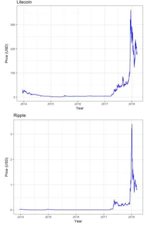
Figure 1: The evolution of daily closing prices in $US for Bitcoin, Litecoin, Dogecoin, Ripple and Feathercoin from 17th of December 2013 until 14th_{of March 2018.}

(28)

The most appropriate models are chosen to implement them for the first stage es-timation of the Dynamic Conditional Correlation model in the next section.

The data used are daily closing prices for the five cryptocurrency series Bitcoin, Litecoin, Dogecoin, Feathercoin and Ripple. It is publicly available online at Coingecko.com. The evolution of prices since December 2013 until March 2018 is shown in figure (1). Dogecoin and Feathercoin have just emerged in 2013 and experience a price increase in late 2013 that fades out in 2014. The most noticeable development is the enormous growth in prices during the hype in mid 2017 which is followed by a short stagnation and another price increase in 2018. All crypto series experienced an extreme multiplication of their value, just before an immense price drop by the end of 2017. Figure (1) thus implicates that the price developments of the five different coins are driven by mutual determinants.

Bitcoin Litecoin Dogecoin Feathercoin Ripple Portfolio Market Cap in USD 155,921,695,042 9,761,938,418 447,366,961 44,076,840 30,826,633,076

-n. obs 1544 1544 1544 1544 1544 1544 Minimum -25.18 -54.72 -94.04 -94.00 -91.34 -52.40 Maximum 28.71 51.44 84.33 72.76 88.13 36.83 Mean 0.15 0.11 0.13 -0.02 0.21 0.14 Median 0.19 -0.08 -0.36 -0.69 -0.17 -0.04 Variance 17.51 38.03 76.22 126.05 59.05 39.05 Stdev 4.18 6.17 8.73 11.23 7.68 6.24 Skewness -0.42 0.34 0.72 0.51 0.84 -0.57 Kurtosis 6.91 14.66 29.88 9.09 34.08 9.09 Jarque-Bera 3128.9 13901 57742 5399.4 75116 5420.7

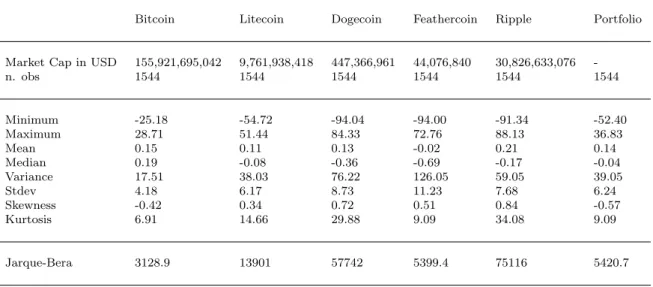
Table 1: Summary Statistics for daily log returns × 100 of cryp-tocurrencies.

Log returns are calculated using: rt= 100×ln(Pt/Pt−1).

Returns are observed until 14th_{of March 2018.}

Market cap is captured at 14th_{of March 2018.}

Jarque-Bera-Test checks for deviation from normality (skewness S different from zero and kurtosisKdifferent from 3): J B=T(S/6 + (k−3)2/24), is distributed asX2_{(2) with 2 degrees of freedom. Its}

critical value at the five-percent level is 5.99 and at the one-percent it is 9.21.

Stylized Facts. Table (1) shows the summary statistics for the cryptocurrency log return series. The log returns are calculated by taking the natural logarithm of the ratio of two consecutive daily closing prices: rt =ln_PP_t−1t ×100. For numerical stability in the statistical softwareR the returns are multiplied by 100. Next to the

(29)

individual series, there is also a return series for an aggregated portfolio calculated. The portfolio return is simply the sum of the individual returns, divided by the number of currencies: rP F,t = 1₅

P5 i=1ri,t.

The data was downloaded on 14thof March 2018. Since the main attempt is to anal-yse the dynamic correlation and multivariate volatility, the datasets are trimmed to the same length with Dogecoin being the youngest currency. This leads to an overall observation span ofT = 1544 for the log returns. The market capitalization in US Dollar reflects the market value and trading volume of the coins. Bitcoin is the most popular currency with the highest market capitalization, followed by Ripple, Litecoin and Dogecoin. Feathercoins market capitalization is the lowest. All currencies except Feathercoin show a positive mean log return. The median of all currencies except for Bitcoin is smaller than zero, which leads to a positive skew-ness in combination with a positive mean. The standard deviation of the returns is in all cases larger than the mean, which is a typical property of highly volatile financial data (Theodossiou, 1998).

It can be noted that Feathercoin has the lowest median return and minimum out of all currencies with the third highest maximum after Dogecoin and Ripple. Also it shows the highest variance. Bitcoin shows the lowest variance and is the only currency that is negatively skewed, which is congruent with the results by Cata-nia and Grassi (2017) and CataCata-nia et al. (2018). Also negative skewness implies that more values bigger than the mean of a distribution were observed, specifically more positive returns. Gkillas and Katsiampa (2018) found Bitcoin to be the least risky coin among the five most popular cryptocurrencies. The other currencies are positively skewed, which has also been shown by Chu et al. (2017). That means that there is more mass on the left side of the density function, i.e. on the negative returns.

The kurtosis k is higher for all currencies than it should be expected for a Normal distribution (k = 3). This is a typical characteristic of financial asset returns since a lot of extreme values are observed and the distribution is highly peaked. The Jarque-Bera-Test for normality (Jarque and Bera, 1987) is rejected for all curren-cies, so the log returns deviate from the Gaussian distribution. For financial data the Central Limit Theorem - stating that the distribution of the sum of a random variable is going to converge to normality for big samples - does not apply in many cases. This is because daily log returns often show higher order moment depen-dencies like asymmetric volatility or conditional heteroscedasticity (Theodossiou, 1998). The Augmented-Dickey-Fuller test (Said and Dickey, 1984), testing the null hypothesis that the time series x has a unit root, is applied to all currencies and

(30)

shows that all log return series are stationary.

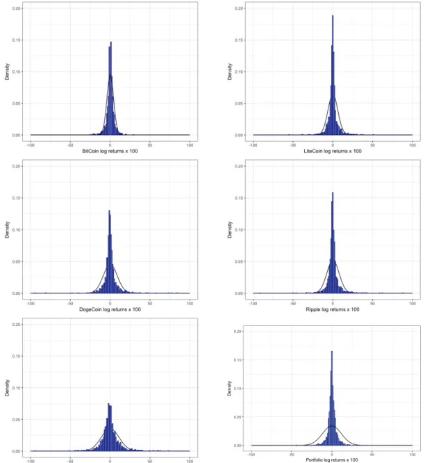
Figure (2) shows the histograms for the density of the log returns. To visualize the deviation from normality, the black line illustrates the theoretical Normal distri-bution, given the same mean and variance. It is visible that Feathercoin has the highest variance and many extreme observations, while Bitcoin has many observa-tions around the return of zero. Dogecoin also shows more heavy-tail behaviour. Figure (3) shows the evolution of the calculated log returns over the available ob-servation span. It shows that Bitcoin has the least risky and volatile behaviour, while Feathercoin and Ripple have a bigger span of variation.

Since the returns for the aggregated portfolio are averaged over the five currencies, the span of the data is smaller, and standard deviation and kurtosis take values on an average level, see table (1). The histogram also shows that there are less extreme observations and more data is located around a return of zero.

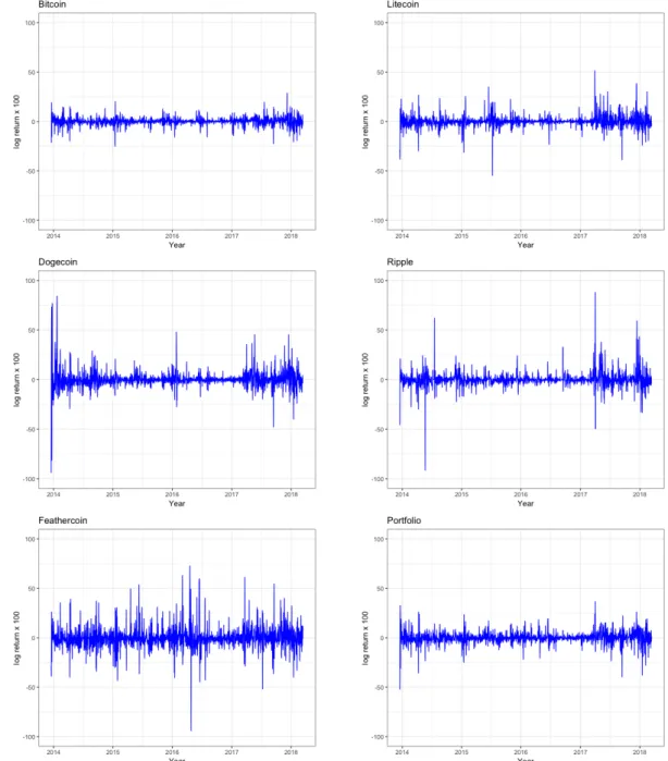
Another typical characteristic of financial time series is the autocorrelation of re-turns. If the evolution of the price experiences an upward or downward dynamic, then the returns are positively correlated for a period of time. Figure (3) shows that for all currencies the returns exhibit periods of higher and lower volatility (volatility clusters). Volatility is extremely high in the period of the cryptocurrency hype dur-ing 2017. Figure (12) in the Appendix shows the Auto Correlation Function of the squared returns. For all currencies there is a significant correlation of returns with the preceeding days that fades out after a couple of days, with some peaks around lag ` = 20 or ` = 30. This structure is typical for ARCH-effects and justifies the application of GARCH-models (Tsay, 2005). Furthermore, the Ljung-Box-Test for serial correlation identifies a dependency within the first ln(T) = ln(1544) = 7.34 lags of the squared innovations ˆat from equation (2), that were calculated by sub-tracting the mean return from the daily return: ˆat =rt−rt (Tsay, 2005).

(31)

Figure 2: Histograms of the log returns of the five cryptocurrencies and the aggregated portfolio in blue.

Log returns are calculated using: rt= 100×ln(Pt/Pt−1).

Black line shows the density of the Normal distribution that would occur for the empirical mean and standard deviation:

x∼N(ri,

p

V ar(ri)).

(32)

Figure 3: The evolution of log returns in $US of Bitcoin, Litecoin, Dogecoin, Ripple, Feathercoin and the aggregated portfolio until 14th

(33)

Univariate GARCH Models. After conditional heteroscedasticity has been de-tected for all five cryptocurrencies, the GARCH models discussed in chapter (4.1) are applied to the univariate log return series. Since the descriptive analysis of the returns has shown fat tails, not only the Gaussian distribution is going to be used for the residual terms but also the Student-t, skewed Student-t and skewed Generalized Error distribution.

All GARCH-type models with different distribution assumptions for the error terms are applied to the univariate time series. The fit is evaluated by diagnostic check-ing and information criteria. More interestcheck-ing, however, is which model is able to provide the best Value at Risk forecasts. The results are going to be used in chap-ter (7) to model the DCC model. Additionally, the GARCH models are going to be applied to the combined portfolio time series consisting of the five currencies. The goal is to find out whether a multivariate approach incorporating the dynamic correlation improves the Value at Risk forecasts for an aggregated portfolio. To model the mean of the time series, a simple ARMA-(1,1) process is defined forµt equivalent to equation (3). When defining the volatility equation (4), the first step is determine to the order of the ARCH effects. This can be done by looking at the PACF of the squared innovations at which can be estimated by the squared series of mean adjusted returns: ˆat =rt−rt. For all five currencies the partial autocorre-lation function reveals significances at higher order lags (around 10 to 100 days). In this case, it is more appropriate to choose the more parsimonious GARCH-model, instead of applying higher order ARCH-models. For the GARCH process usually a lower order model like the GARCH-(1,1) or GARCH-(2,1) is appropriate in most applications (Tsay, 2014).

A GARCH-(1,1) process is defined for the standard GARCH, iGARCH, iGARCH, gjr-GARCH, apARCH and csGARCH models with the Normal, Student-t, skewed Student-t, and skewed Generalized Error distribution for each logarithmic return series of the five currencies. The models are estimated via Maximum-Likelihood.

(34)

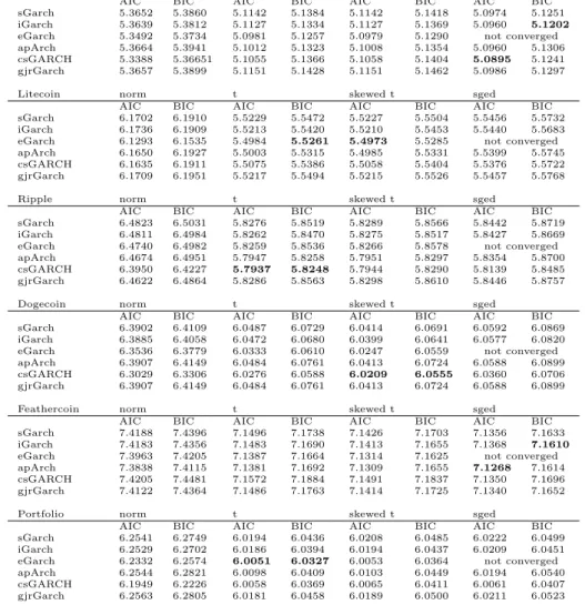
Bitcoin norm t skewed t sged

AIC BIC AIC BIC AIC BIC AIC BIC sGarch 5.3652 5.3860 5.1142 5.1384 5.1142 5.1418 5.0974 5.1251 iGarch 5.3639 5.3812 5.1127 5.1334 5.1127 5.1369 5.0960 5.1202 eGarch 5.3492 5.3734 5.0981 5.1257 5.0979 5.1290 not converged apArch 5.3664 5.3941 5.1012 5.1323 5.1008 5.1354 5.0960 5.1306 csGARCH 5.3388 5.36651 5.1055 5.1366 5.1058 5.1404 5.0895 5.1241 gjrGarch 5.3657 5.3899 5.1151 5.1428 5.1151 5.1462 5.0986 5.1297 Litecoin norm t skewed t sged

AIC BIC AIC BIC AIC BIC AIC BIC sGarch 6.1702 6.1910 5.5229 5.5472 5.5227 5.5504 5.5456 5.5732 iGarch 6.1736 6.1909 5.5213 5.5420 5.5210 5.5453 5.5440 5.5683 eGarch 6.1293 6.1535 5.4984 5.5261 5.4973 5.5285 not converged apArch 6.1650 6.1927 5.5003 5.5315 5.4985 5.5331 5.5399 5.5745 csGARCH 6.1635 6.1911 5.5075 5.5386 5.5058 5.5404 5.5376 5.5722 gjrGarch 6.1709 6.1951 5.5217 5.5494 5.5215 5.5526 5.5457 5.5768

Ripple norm t skewed t sged

AIC BIC AIC BIC AIC BIC AIC BIC sGarch 6.4823 6.5031 5.8276 5.8519 5.8289 5.8566 5.8442 5.8719 iGarch 6.4811 6.4984 5.8262 5.8470 5.8275 5.8517 5.8427 5.8669 eGarch 6.4740 6.4982 5.8259 5.8536 5.8266 5.8578 not converged apArch 6.4674 6.4951 5.7947 5.8258 5.7951 5.8297 5.8354 5.8700 csGARCH 6.3950 6.4227 5.7937 5.8248 5.7944 5.8290 5.8139 5.8485 gjrGarch 6.4622 6.4864 5.8286 5.8563 5.8298 5.8610 5.8446 5.8757 Dogecoin norm t skewed t sged

AIC BIC AIC BIC AIC BIC AIC BIC sGarch 6.3902 6.4109 6.0487 6.0729 6.0414 6.0691 6.0592 6.0869 iGarch 6.3885 6.4058 6.0472 6.0680 6.0399 6.0641 6.0577 6.0820 eGarch 6.3536 6.3779 6.0333 6.0610 6.0247 6.0559 not converged apArch 6.3907 6.4149 6.0484 6.0761 6.0413 6.0724 6.0588 6.0899 csGARCH 6.3029 6.3306 6.0276 6.0588 6.0209 6.0555 6.0360 6.0706 gjrGarch 6.3907 6.4149 6.0484 6.0761 6.0413 6.0724 6.0588 6.0899 Feathercoin norm t skewed t sged

AIC BIC AIC BIC AIC BIC AIC BIC sGarch 7.4188 7.4396 7.1496 7.1738 7.1426 7.1703 7.1356 7.1633 iGarch 7.4183 7.4356 7.1483 7.1690 7.1413 7.1655 7.1368 7.1610 eGarch 7.3963 7.4205 7.1387 7.1664 7.1314 7.1625 not converged apArch 7.3838 7.4115 7.1381 7.1692 7.1309 7.1655 7.1268 7.1614 csGARCH 7.4205 7.4481 7.1572 7.1884 7.1491 7.1837 7.1350 7.1696 gjrGarch 7.4122 7.4364 7.1486 7.1763 7.1414 7.1725 7.1340 7.1652 Portfolio norm t skewed t sged

AIC BIC AIC BIC AIC BIC AIC BIC sGarch 6.2541 6.2749 6.0194 6.0436 6.0208 6.0485 6.0222 6.0499 iGarch 6.2529 6.2702 6.0186 6.0394 6.0194 6.0437 6.0209 6.0451 eGarch 6.2332 6.2574 6.0051 6.0327 6.0053 6.0364 not converged apArch 6.2544 6.2821 6.0098 6.0409 6.0103 6.0449 6.0194 6.0540 csGARCH 6.1949 6.2226 6.0058 6.0369 6.0065 6.0411 6.0061 6.0407 gjrGarch 6.2563 6.2805 6.0181 6.0458 6.0189 6.0500 6.0211 6.0523

Table 2: AIC and BIC for the estimated GARCH-type models. µt is modelled via an ARMA-(1,1) process. σt is modelled via a

GARCH-type process of order (1,1). T=1544.

Lowest AICs and BICs per group are written inboldletters.

Table (2) shows the AIC and BIC for the fitted GARCH-type models with differ-ent distribution assumptions for the innovations. The models that performed best for every currency or the portfolio according to the Akaike or Bayes Information Criterion are written in bold letters. As a first result, it shows that the Gaussian distribution for the error terms is outperformed by its heavy-tailed alternatives. AIC and BIC indicate a lower fit here over all different currencies. The eGARCH in combination with the skewed Generalized Error distribution showed convergence problems for all currencies that remained even after several adjustments of solver options.

For Bitcoin and Feathercoin, the skewed Generalized Error distribution delivers the best fit for almost all models. AIC is lowest for the csGARCH, nearly followed by the iGARCH for Bitcoin and the apARCH for Feathercoin. This is supported by

(35)

the findings by Katsiampa (2017), who also showed that the component-standard GARCH provides the best fit to model Bitcoins volatility according to information criteria. The quantile-to-quantile plot and the ACF of the squared residuals indi-cate a good fit. For Litecoin, the skewed Student-t distribution seems to be most appropriate and works best along with the eGARCH model. For Dogecoin, the eGARCH, csGARCH and apARCH deliver the best information criteria with the apARCH showing most reasonable plots in model diagnostics on the error terms. The apARCH with Student-t distribution works best for Ripple according to resid-ual plots. However, the skew parameter for the equivalent model with the skewed Student-t distribution is significant. For the aggregated portfolio, the information criteria show that the return series is best modelled via the Student-t distribution with an eGARCH, however, the shape parameter for the corresponding model with a skewed Student-t distribution is also significant and reports good information criteria and residual plots.

In general, the univariate GARCH models show that there is a need for skewed distributions to model the volatility process of the currencies. The apARCH, cs-GARCH and ecs-GARCH models seem to work best according to AIC and BIC, however, there is usually only a slight difference between the models if the right distribution for error terms is chosen. Bitcoin is most accurately modelled via a csGARCH, which is supported by the findings of Katsiampa (2017). Bitcoin and Feathercoin show a good model fit if the innovations are modelled via the skewed Generalized error distribution. It should be noted that the apARCH and eGARCH are more parsimonious than the csGARCH which contains a time-varying intercept for the conditional variance. However, the models should also be evaluated via their performance on Value at Risk forecasting. The choice of the right distribution assumption for the error terms is of great importance here.

(36)

Value at Risk. Now it is interesting to find out which of the models produce the best Value at Risk forecasts.

Figure 4: Outline for the 1-day-ahead forecast.

The time line shows the training data set of length T=800 in black and the rolling out-of-sample forecast of length T=744 in green. Red arrows indicate the observations included in the three parameter re-estimations (recursive window).

Since the altcoin market is quite young, the length of the return series is short in comparison to other traditional currencies or indices. Therefore, it is more appro-priate to estimate the rolling forecast based on a recursive window. That means all past observations are included in the estimation of the current parameters in con-trast to a moving window where all the previous data is used for the first estimation and then moved by a pre-defined length for every forecast.

Figure (4) shows the outline for the forecast. The rolling forecast starts att= 800, which leaves 744 one-day-ahead forecasts. The parameters are refitted every 300 days, thus the model parameters are refitted three times. The red arrows show the past observations that are included for the estimation of the model parameters. Within the refitting period, the parameters are fixed but data is updated for every trading day.

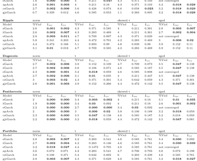
Table (3) reports the backtesting results for the Value at Risk forecast. VaR is calculated for every GARCH model and distribution at the 1%-, and 5%-level and evaluated via VaR backtesting described in section (4.4). The percent violations show how many times the returns dropped below the VaR forα= 0.01 andα= 0.05 predicted by the model in relation to the total number of forecasts. Additionally, the p-values for the tests of conditional and unconditional coverage are reported. The models where the tests for conditional or unconditional coverage were rejected at the 95% confidence level are written in bold.

(37)

VaR 1%

Model %Viol Luc Lcc %Viol Luc Lcc %Viol Luc Lcc %Viol Luc Lcc

sGarch 2.3 0.006 0.017 1.3 0.37 0.584 0.9 0.87 0.923 0.8 0.583 0.819 iGarch 2.3 0.003 0.007 1.2 0.578 0.767 0.9 0.87 0.923 0.8 0.583 0.819 eGarch 2.3 0.003 0.007 0.7 0.339 0.612 0.5 0.165 0.373 not converged

apArch 2.4 0.001 0.003 0.4 0.063 0.175 0.4 0.063 0.175 0.5 0.165 0.373 csGarch 2 0.014 0.037 1.3 0.37 0.585 1.5 0.221 0.41 0.8 0.853 0.819 gjrGarch 2.2 0.006 0.017 1.2 0.578 0.767 0.9 0.87 0.923 0.7 0.339 0.612

Litecoin norm t skewed t sged

apArch 0.7 0.339 0.612 0.5 0.165 0.373 0.7 0.339 0.612 0.5 0.165 0.373 csGarch 0.9 0.87 0.923 1.2 0.878 0.787 1.6 0.123 0.125 0.5 0.165 0.373 gjrGarch 0.7 0.339 0.612 1.1 0.838 0.898 1.1 0.383 0.895 0.5 0.165 0.373

Ripple norm t skewed t sged

Dogecoin norm t skewed t sged

Feathercoin norm t skewed t sged

Portfolio norm t skewed t sged

VaR 5%

sGarch 5.1 0.893 0.142 6.2 0.153 0.028 6 0.203 0.027 5 0.973 0.118 iGarch 4.8 0.839 0.289 6.2 0.153 0.028 6 0.203 0.027 4.8 0.839 0.095 eGarch 5.1 0.893 0.142 6.2 0.203 0.027 5.8 0.341 0.078 not converged

apArch 4.8 0.839 0.289 5.6 0.428 0.074 5.6 0.428 0.074 4.7 0.709 0.073 csGarch 5.1 0.893 0.382 6.6 0.058 0.023 6.6 0.058 0.023 4.8 0.839 0.289 gjrGarch 5 0.973 0.339 6.3 0.113 0.009 6 0.203 0.027 4.8 0.839 0.095

Litecoin norm t skewed t sged