Default cycles

ADEMU WORKING PAPER SERIES

Default Cycles

Wei Cui

Leo Kaas

Abstract

Recessions are often accompanied by spikes of corporate default and prolonged declines of business credit. This paper argues that credit and default cycles are the outcomes of variations in self-fulfilling beliefs about credit market conditions. We develop a tractable macroeconomic model in which leverage ratios and interest spreads are determined in optimal credit contracts that reflect the expected default risk of borrowing forms. We calibrate the model to evaluate the impact of sunspots and fundamental shocks on the credit market and on output dynamics. Self-fulfilling changes in credit market

expectations trigger sizable reactions in default rates and generate endogenously persistent credit and output cycles. All credit market shocks together account for about 50% of the variation of U.S. output growth during 1982-2015.

JEL classification: E22, E32, E44, G12

Keywords: Firm default; Financing constraints; Credit Spreads; Sunspots

___________________

Ŧ_{Department of Economics, University College London; Centre for Macroeconomics, UK. Email: [email protected]} ŧ _{Department of Economics, University of Konstanz, 78457 Konstanz, Germany. Email: [email protected]}

Acknowledgments

We thank Lars Hansen, Patrick Kehoe, Dominik Menno, Alexander Monge-Naranjo, Franck Portier, and Morten Ravn for helpful comments and discussions, and seminar and conference audiences at CEMFI, Chinese University of Hong Kong, Frankfurt, Hong Kong Monetary Authority, Hong Kong University, Konstanz, Manchester, Oxford, SFU, St. Gallen, Tsinghua, and UCL for their comments. Leo Kaas thanks the German Research Foundation (grant No. KA 442/15) for financial support. Wei Cui thanks the Centre for Macroeconomics (grant No. ES/K002112/1), the ADEMU European Horizon 2020 (grant No. 649396), and the HKIMR for financial support. The usual disclaimer applies.

The ADEMU Working Paper Series is being supported by the European Commission Horizon 2020 European Union funding for Research & Innovation, grant agreement No 649396.

This is an Open Access article distributed under the terms of the Creative Commons Attribution License Creative Commons Attribution 4.0 International, which permits unrestricted use, distribution and reproduction in any medium provided that the original work is properly attributed.

1

Introduction

Many recessions are accompanied by substantial increases of corporate default rates and credit spreads, together with declines of business credit. On the one hand, corporate defaults tend to be clustered over prolonged episodes which gives rise to persistent credit cycles (see e.g. Giesecke et al. (2011)). Such clustering of default can only partly be explained by observable firm-specific or macroeconomic variables, but is driven by unobserved factors that are correlated across firms and over time (Duffie et al. (2009)). On the other hand, credit spreads tend to lead the cycle and are not fully accounted for by expected default. Moreover, less than half of the volatility of credit spreads can be explained by expected default losses; instead, it is the “excess premium” on corporate bonds that has the strongest impact on investment and output (Gilchrist and Zakrajˇsek (2012)).

This paper examines the joint dynamics of firm default, credit spreads and output, using a tractable dynamic general equilibrium model in which firms issue defaultable debt. We argue that default rates in such economies are susceptible to self-fulfilling beliefs over credit conditions. States of low default and good credit conditions can alternate between states of high default and bad credit conditions. Stochastic variation of self-fulfilling beliefs play a key role in accounting for the persistent dynamics of default rates and their co-movement with macroeconomic variables.

To illustrate our main idea, we present in Section 3 a simple partial-equilibrium model of firm credit with limited commitment and equilibrium default. Leverage and the interest rate spread depend on the value that borrowing firms attach to future credit market conditions which critically impacts the firms’ default decisions, and hence is taken into account in the optimal credit contract. This credit market value is a forward-looking variable which reacts to self-fulfilling expectations. A well-functioning credit market with a low interest rate and a low default rate is highly valuable for firms, and this high valuation makes credit contracts with few defaults self-enforcing. Conversely, a weak credit market with a higher interest rate and more default is valued less by firms, and therefore it cannot sustain credit contracts that prevent high default rates.

After this illustrative example, we build in Section 4 a general-equilibrium model in order to analyze the role of self-fulfilling expectations and fundamental shocks for the dynamics of default rates, spreads and their relationships with the aggregate economy. Credit constraints, spreads, default rates, and aggregate productivity are all endogenous outcomes of optimal debt contracts. As in the simple model, leverage ratios and default rates depend on the value that borrowers attach to future credit market conditions which is susceptible to changes of self-fulfilling beliefs. Aggregate productivity is determined by the allocation of capital among

firms which itself depends on current leverage ratios and on past default events. When credit is tightened or when more firms opt for default, less capital is operated by the most productive firms so that aggregate productivity and output fall.

Firms in our model differ in productivity and in their access to the credit market. High-productivity firms with a good credit standing borrow up to an endogenous credit limit at an interest rate which partly reflects the expected default loss and which also includes an excess interest premium. This premium, which may itself be subject to aggregate shocks, is a shortcut to account for the so-called “credit spread puzzle” according to which actual credit spreads are larger than expected default losses (e.g., Elton et al. (2001) and Huang and Huang (2012)). We also allow the recovery rate to fluctuate which affects the expected default loss and hence takes a direct impact on leverage and on the predicted component of the credit spread.

If a firm opts for default, a fraction of its assets can be recovered by creditors. After default, the firm’s owner may continue to operate a business (possibly under a different name), but she loses the good credit standing and hence remains temporarily excluded from the credit market. Notice that net worth of firms with credit market access is endogenous, and aggregate productivity and factor demand depend on the borrowing capacity (net worth multiplied by the leverage ratio) of firms. Then, periods of high default can have a long-lasting impact on credit and output. In the next section we use a simple VAR model to show that shocks to the default rate, which are orthogonal to credit spreads and recovery rates, have indeed a negative impact on output growth. Modeling the default cycle is therefore crucial for the overall macroeconomic dynamics.

In Section 5 we calibrate this model and show that it responds to changes in self-fulfilling beliefs about credit market conditions. These belief changes can be induced by fundamental shocks to the real or to the financial sector (i.e., shocks to the recovery rate, to the excess premium, or to aggregate productivity), but they can also be completely unrelated to funda-mentals (sunspot shocks). We show that variations in self-fulfilling beliefs are crucial for the dynamics of default rates. An adverse sunspot shock raises the default rate and depresses leverage. Additionally, sunspots are also tied to shocks to the recovery rate, to the excess premium, and to aggregate productivity. That is why these fundamental shocks also gen-erate reactions of default rates. Finally, recovery shocks are important for credit flows and output growth.

Although different shocks in our model can be called “financial shocks”, the generated equilibrium responses are significantly different from each other, highlighting the complex dimensions of financial frictions. Our model links these dimensions in a tractable model framework, and the model estimation suggests that all three financial shocks together

ex-plain output dynamics since 1982 rather well and account for about 50% of output growth volatility, of which about 40% are induced by changes in credit market expectations.

Our work relates to a number of recent contributions analyzing the macroeconomic im-plications of credit spreads and firm default. Building on Bernanke et al. (1999), Christiano et al. (2014) introduce risk shocks in a quantitative business-cycle model and show that these shocks not only generate countercyclical spreads but also account for a large fraction of macroeconomic fluctuations. Miao and Wang (2010) include long-term defaultable debt in a macroeconomic model with financial shocks to the recovery rate. In line with empirical evidence, they find that credit spreads are countercyclical and lead output and stock returns. Gomes and Schmid (2012) develop a macroeconomic model with endogenous default of het-erogeneous firms and analyze the dynamics of credit spreads. Gourio (2013) is motivated by the volatility of the excess bond premium and argues that time-varying risk of rare de-pressions (disaster risk) can generate plausible volatility of credit spreads and co-movement with macroeconomic variables. Self-fulfilling expectations do not matter in all these contri-butions which differ from our model in that default incentives do not depend on expected credit conditions. Also, these papers do not allow for a link between the credit market and aggregate factor productivity.1

Our work further builds on a literature on self-fulfilling expectations and multiplicity in macroeconomic models with financial market imperfections. Most closely related is Azariadis et al. (2016) who show that sunspot shocks account for the procyclical dynamics of unsecured credit. As in this paper, equilibrium indeterminacy arises due to a dynamic complementarity in borrowers’ valuation of credit market access. Harrison and Weder (2013), Benhabib and Wang (2013), Liu and Wang (2014) and Gu et al. (2013) also show how equilibrium indeterminacy and endogenous credit cycles arise in credit-constrained economies.

None of these papers addresses default and credit spreads. Notice that default in librium is important, although the average default rate might be low. This is because equi-librium default imposes an externality on others who choose not to default: Credit contracts and the associated leverage ratios reflect these potential default risks. Furthermore, the variation in default rates in our model is almost entirely caused by variations in self-fulfilling beliefs. This fact can be used to back out shocks that impact beliefs, and we show that these shocks are quantitatively important for the overall volatility of output growth.

The co-existence of equilibria with high (low) interest rates and high (low) default rates relates to a literature on self-fulfilling sovereign debt crises. In a two-period model, Calvo

1_{Khan et al. (2016) introduce firm dynamics and default risk in a macroeconomic model and show that}

countercyclical default affect the capital allocation among firms, which amplifies and propagate real and financial shocks. Unlike our model, there is no role for self-fulfilling expectations.

(1988) shows how multiple equilibria emerge from a positive feedback between interest rates and debt levels. Lorenzoni and Werning (2013) extend this idea to a dynamic setting to study the role of fiscal policy rules and debt accumulation for the occurrence of debt crises. On the other hand, Cole and Kehoe (2000) find that self-fulfilling debt crises occur because governments cannot roll over their debt (cf. Conesa and Kehoe (2015) Aguiar et al. (2013)). Our mechanism for multiplicity is different from these contributions by emphasizing the role of expectations about future credit conditions. We further focus on strategic default of borrowers in general equilibrium.

2

VAR Evidence

In this section we examine the separate roles of the default rate, credit spreads and the recovery rate for output dynamics on the basis of a vector autoregression model. We obtain data for the recovery rate and the all-rated default rate for Moody’s rated corporate bonds, covering the period 1982–2015, all in percentage terms, and we use the credit spread index developed by Gilchrist and Zakrajˇsek (2012) that is representative for the full corporate bond market.2 Output is defined as the sum of private consumption and private investment in the U.S. national accounts. Output growth refers to the growth rate of real per capita output.

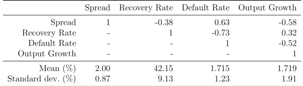
Table 1: Summary Statistics

Spread Recovery Rate Default Rate Output Growth

Spread 1 -0.38 0.63 -0.58 Recovery Rate - 1 -0.73 0.32 Default Rate - - 1 -0.52 Output Growth - - - 1 Mean (%) 2.00 42.15 1.715 1.719 Standard dev. (%) 0.87 9.13 1.23 1.91

Table 1 shows the correlation structure of these four variables. As expected, the default rate and the credit spread are highly positively correlated, and both of them are counter-cyclical. The recovery rate is highly negatively correlated with the default rate, but less with the credit spread and it is mildly procyclical.

In order to further understand their relationships, we order the four variables according to [spread, recovery, default, Output Growth]’ and estimate a structural VAR model using 2_{Moody’s data are obtained from the 2015 annual report published by Moody’s Investors Service. The}

recovery rate is measured by the post-default bond price for one dollar repayment. Regarding the spread series, we consider annual averages of the monthly series, updated until 2015 (see Simon Gilchrist’s website http://people.bu.edu/sgilchri/Data/data.htm).

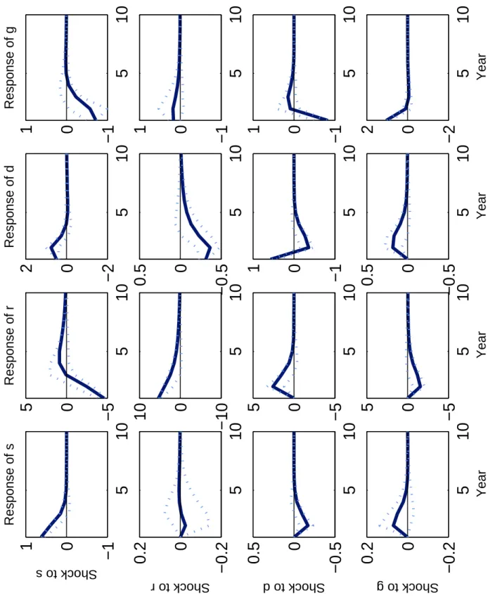
Figure 1: VAR Evidence. Note: “s”: credit spread, “r”: recovery rate, “d”: default rate, and “g”: output growth rate. All variables are in percentage terms. The dotted lines are 5% and 95% intervals

5

10

−1

0

1

5

10

−5

0

5

5

10

−2

0

2

5

10

−1

0

1

5

10

−0.2

0

0.2

5

10

−10

0

10

5

10

−0.5

0

0.5

5

10

−1

0

1

5

10

−0.5

0

0.5

5

10

−5

0

5

5

10

−1

0

1

5

10

−1

0

1

5

10

−0.2

0

0.2

5

10

−5

0

5

5

10

−0.5

0

0.5

5

10

−2

0

2

a standard Cholesky decomposition. We rank financial market variables before the macro variable. Notice that default is put as the last of financial market variables, so that exogenous shocks to default should have the least impact. Different orderings of financial variables do not significantly change the results. Figure 1 presents impulse responses functions from the VAR estimation and 90% confidence bands from 1000 boostrap draws.

An immediate observation is that a shock that raises default rate on impact does not lead to the rise of spread in the 2nd period. The subsequent fall of default pushes down the spread, but the magnitude of fall in spread is smaller. At the same time, it pushes up the recovery rate and depresses real output growth. Notice that even if one considers the increase of recovery rate, the fall of spreads is still smaller than the fall of default rate.

In the model that we consider below, the default rate is most strongly affected by changes in self-fulfilling beliefs. Believes into higher default rates lead to a cut in lending and higher credit spreads. The fall in credit induces a decline in economic activity. Since lending is reduced, given the constant recovery ability, lenders can recover more per unit of lending, which explains why the measured recovery rate goes up.

This VAR exercise shows that the recovery rate, credit spreads, and the default rate seem to have a non-trivial relationship. Different shocks in the financial market can cause different responses both in the financial market itself and in the real economy. This finding motivates us to develop a macroeconomic model with borrowing constrained firms and endogenous default, which takes into account different mechanisms by which default, recovery rates, and spreads are affected by macroeconomic shocks. Credit market conditions impact firms with different productivity levels so that the real economy responds to changes in the credit market.

3

An Illustrative Example

We present a simple partial equilibrium model to illustrate how default rates, credit spreads and leverage can vary in response to changes in self-fulfilling expectations. The model has a large number of firms who live through infinitely many discrete periods t ≥0. Firm owners are risk-averse and maximize discounted expected utility

E0 X t≥0 βt (1−β) logct−ηt

where ct is consumption (dividend payout) in period t, β < 1 is the discount factor, and

ηt is a default loss that materializes only when the firm defaults in period t.3 For example, the default loss may reflect the additional labor effort of the firm owner in a default event.4 The default loss is idiosyncratic and stochastic: with probability p it is zero, otherwise it is ∆>0. Hence in any given period, fraction pof the firms are more prone to default.

All firms are endowed with one unit of net worth in period zero and they have access to a linear technology that transforms one unit of the consumption good in periodtinto Π units of the good in periodt+ 1. Firms may obtain one-period credit from perfectly competitive and risk-neutral investors who have an outside investment opportunity at rate of return ¯R <Π. Although firms cannot commit to repay their debt, there is a record-keeping technology that makes it possible to exclude defaulting firms from all future credit. That is, if a firm decides to default, it is subject to the default utility loss (if any) in the default period and it may not borrow in all future periods.

Investors offer standard debt contracts that specify the interest rate R and the volume of debtb. Competition between investors ensures that the offered contracts (R, b) maximize the borrower’s utility subject to the investors’ participation constraint. The latter requires that the expected return equals the outside return ¯R per unit of debt.

In recursive notation, a firm owner’s utility V(ω) depends on the firm’s net worth ω and satisfies the Bellman equation

V(ω) = max c,s,(R,b)(1−β) log(c) +βEmax n V(ω0), Vd(ω0_d)−η o , s.t. (1) c=ω−s , ω0 = Π(s+b)−Rb , ω_d0 = Π(s+b) , E(R·b) = ¯R·b .

The firm owner chooses consumption, savings, and a particular credit contract (R, b), subject to the investors’ participation constraint. Next period, she can choose to repay and obtain net worthω0; she can also choose to default and obtain net worth ω0_d, in which case she has to bear the default cost. The second maximization expresses the optimal ex-post default choice at the beginning of the next period, and the expectation operator _E is over the

3_{The utility cost with log utility ensure that there is closed form solution for binary choice of default}

and no-default. See Cui (2014) for a similar treatment of binary choice of selling capital or being inactive.

4_{Alternatively, we may assume in this example, as well as in the full macro model of the next section,}

that a defaulting firm’s net worth is subject to a real default cost shock. This alternative model has the same credit market equilibrium but slightly different aggregate dynamics. Details are available upon request.

firm’s realization of the default cost η ∈ {0,∆}. The defaulting firm is further punished by exclusion from future credit: Vd_{(.) is the utility value of a firm with a default history, which} satisfies the recursion

Vd(ω) = max c,s (1−β) log(c) +βV d_(ω0 ) , s.t. (2) c=ω−s , ω0 = Πs .

We show in the Appendix A (proof of Proposition 2) that all firms save s = βω and that value functions take the simple forms

V(ω) = log(ω) +V , Vd(ω) = log(ω) +Vd ,

where V and Vd _{are independent of the firm’s net worth. We write v ≡ V −V}d _{to express} the surplus value of access to credit; it is a forward-looking variable that reflects expected credit conditions. Using this notation, we can write the value function asV(ω) = maxs(1−

β) log(ω−s) +β[Vd+U(s)] where U(s) is the surplus value of the optimal credit contract for a firm with savings s. It solves the problem

U(s)≡max (R,b)Emax n log[Π(s+b)−Rb] +v,log[Π(s+b)]−ηo s.t. ¯ Rb=_E(Rb) =      Rb if log[Π(s+b)−Rb] +v ≥log[Π(s+b)] ,

(1−p)Rb if log[Π(s+b)]>log[Π(s+b)−Rb] +v ≥log[Π(s+b)]−∆ ,

0 else.

The participation constraint captures three possible outcomes. In the first case, the firm repays for any realization of the default loss in which case investors are fully repaid Rb. In the second case, the firm only repays when the default loss is positive, which is reflected in the expected payment (1−p)Rb. In the third case, the firm defaults with certainty.

It is straightforward to characterize the optimal contract. Proposition 1. Suppose that the parameter condition

(e∆_−1)(1−p) e∆_{−1 +p} < ¯ R Π < (e(1−p)∆_−e−p∆_)(1−p) e(1−p)∆₋₁ (3)

that

(i) If v ∈ [¯v, vmax_{), the optimal contract is (R, b) = ( ¯R, b(s)) with debt level and borrower} utility b(s) = s Π(1−e −v₎ ¯ R−Π(1−e−v₎ , U(s) = log h R¯Πs ¯ R−Π(1−e−v₎ i .

(ii) If v ∈ [0,v¯), the optimal contract is (R, b) = ( ¯R/(1− p), b(s)), with debt level and borrower utility b(s) = s Π(1−p)(1−e −v−∆₎ ¯ R−Π(1−p)(1−e−v−∆₎ , U(s) = log h R¯Πs ¯ R−Π(1−p)(1−e−v−∆₎ i −(1−p)∆.

Proof. See Appendix A.

If expected credit conditions are good enough,v ≥v¯, the threat of credit market exclusion is so severe that no firm defaults in the optimal contract. The corresponding debt level is the largest one that prevents default of firms with zero default loss whose binding enforcement constraint is log[Π(s +b) −Rb] + v = log[Π(s +b)]. A feasible solution to the optimal contracting problem further requires that debt is finite which necessitates v < vmax.

Alternatively, if expected credit conditions are not so good, v <v¯, the optimal contract allows for partial default since it is then relatively costly to prevent default of all firms. Instead, fraction p of firms default in the optimal contract, whereas firms with positive default cost are willing to repay which is ensured by log[Π(s+b)−Rb]+v = log[Π(s+b)]−∆. The parameter conditions (3) imply that both outcomes are optimal for different values of expected credit conditions. If one of these inequalities fails, either no default (i) or partial default (ii) is the optimal contract for all feasible values of v.

Expected credit conditionsv depend themselves on the state of the credit market and are determined in a stationary equilibrium by the forward-looking Bellman equations (1) and (2). After substitution of U(s) from Proposition 1, it is straightforward to show that the value difference v =V −Vd _{satisfies the fixed-point equation}

v =f(v)≡    βlogh_{R¯−Π(1−}R¯ _e−v₎ i if v ≥v ,¯ βnlogh R¯ ¯ R−Π(1−p)(1−e−v−∆₎ i −(1−p)∆o if v <v .¯

Any solution of this equation constitutes a stationary equilibrium of this economy. Under the conditions of Proposition 2, it can be verified thatf is increasing and continuous, and it satisfies f(0) >0 and f(v)→ ∞ for v →vmax_{. This shows that, generically, the fixed-point} equation has either no solution, or two solutions. Moreover, if f(¯v) <v¯ holds, there is one

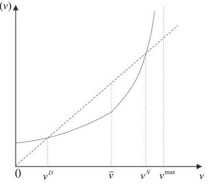
Figure 2: Co-existence of Default and No-Default Equilibria

0

v

v

v

v

)

(

v

f

v

equilibrium at vD _{< v¯ which involves default and a positive interest spread together with} another equilibrium at vN _{>v¯which has no default and a zero spread (see Figure 2). This} result is summarized as follows.5

Proposition 2. Suppose that parameters satisfy

R¯ ¯ R−Π(1−e−¯v₎ β < Π[1−(1−p)e −p∆_] Π−R¯+e(1−p)∆_{( ¯R−Π(1−p))} , (4)

as well as condition (3). Then there are two stationary credit market equilibria vD _{< v}N such that default rates and interest spreads are positive at vD _{and zero at v}N_.

Proof. See Appendix A.

The main insight of this proposition is that the state of the credit market is a matter of self-fulfilling expectations. A well-functioning credit market with a low interest rate and a low default rate is highly valuable for firms, and this high valuation makes credit contracts without default self-enforcing. Conversely, a weak credit market with a higher interest rate and more default is valued less by the firms, and therefore it cannot sustain credit contracts that prevent default.

5_{If the parameter condition (4) (which is equivalent to f(¯v) < v¯) fails, there can exist at most two}

equilibria with default, or at most two equilibria without default. Since function f is convex and kinks upwards at ¯v, there cannot be more than two equilibria.

Although the two equilibria are clearly ranked in terms of default rates, interest rates and utility, it is worth noticing that leverage, defined as the debt-to-equity ratio b(s)/s, can be higher or lower in the no-default state compared to the default state. On the one hand, the lower interest rate and the higher credit market valuation at the no-default equilibrium permit a greater leverage. On the other hand, preventing default of all firms requires a tighter borrowing constraint compared to the one that induces only firms with high default costs to repay.6

The additional parameter condition (4) of Proposition 2 is fulfilled whenever the discount factor β is low enough (because the fraction on the right-hand side is strictly greater than one). Conversely, the condition fails ifβ is sufficiently large.7 In other words, a prerequisite for weak credit markets is that future consumption is discounted enough.

While the previous analysis describes stationary equilibria, this partial equilibrium model also gives rise to self-fulfilling sunspot cycles in which the economy fluctuates perpetually between states of positive spreads and default and states with zero spreads and no default:8 Proposition 3. Under the condition of Proposition 2, there exists a stochastic equilibrium in which the economy alternates between states with positive defaultv1 <v¯and states without default v2 >¯v with transition probability π∈(0,1).

Proof. See Appendix A.

4

The Macroeconomic Model

We extend the insights of the previous section to a dynamic general equilibrium economy. The main departures from the partial model are as follows: (i) the safe interest rate is determined in credit market equilibrium; (ii) lenders can recover some of their exposure in default events; (iii) defaulters are not permanently excluded; (iv) due to idiosyncratic 6_{To give a numeric example, setβ = 0.9, Π = 1, ¯R= 0.92, p= 0.1, and two values of the default loss,}

∆ = 0.2 and ∆ = 0.4. For both values of ∆, there is a no-default equilibrium at vN _{≈0.43 with leverage}

b/s≈0.61. For ∆ = 0.2, the default equilibrium atvD _{≈0.11 has lower leverage b/s≈0.35. For ∆ = 0.4,}

leverage at the default equilibriumvD_{≈0.2 isb/s≈0.79. Hence, the default equilibrium can havehigher}

leverage than the no-default equilibrium: the greater default loss relaxes the borrowing constraint which is imposed to preclude default of high-cost firms, while permitting default of the other firms.

7_{In this limiting case infinite debt levels would become sustainable, so that this partial model has no}

equilibrium at the given (low) interest rate ¯R < Π. In the general-equilibrium model of the next section there always exists an equilibrium since the endogenous interest rate would rise whenβ becomes sufficiently large.

8_{Since the relationship between credit market expectations in periods t and t+ 1 is monotonic (see}

Figure 2), there are no deterministic cycles. The existence of sunspot cycles rests on a continuity argument (cf. Chiappori and Guesnerie (1991)) in the presence of multiple steady states; see the proof of Proposition 3 in the Appendix.

productivity shocks the credit market impacts aggregate factor productivity; (v) we introduce aggregate shocks to study business-cycle implications. These include fundamental shocks (technology and financial variables) as well as sunspot shocks.

4.1

The Setup

Firms and Workers

The model has a unit mass of infinitely-lived firm owners with the same preferences as in the previous section: period utility is (1−β) log(c)−η wherecis consumption and β is the discount factor. The idiosyncratic default loss η is distributed with cumulative function G

which is assumed to have no mass points.

All firms operate a production technology which produces output (consumption and investment goods) y = (zk)α_(A

t`)1−α from inputs capital k and labor ` with capital share

α ∈ (0,1). At is time-varying aggregate productivity that grows over time and is hit by exogenous productivity shocks,9 _logA

t=µAt +logAt−1, whereµA_t follows a stationary process with mean µA_.

Firms can have high or low capital productivityz, and the idiosyncratic productivity state follows an i.i.d process. Specifically, a firm obtains high productivity zH _{with probability π} and low productivity zL=γzH with 1−π. To simplify algebra, we assume that the capital productivity shock affects the stock of capital (rather than the capital service), so that the firm’s capital stock at the end of the period is (1−δ)zk, whereδ is the depreciation rate.

Next to firm owners, the economy includes a mass of workers who supply laborl and who consume their labor earnings c=wl. Their preferences are represented by a modified GHH utility function that allows for balanced growth paths,uct−

Atκlt1+ν

1+ν

, whereuis increasing and concave, and κ, ν >0.10 _{Workers are hand-to-mouth and supply labor according to}

wt/At=κltν . (5) That workers are hand-to-mouth consumers is not a strong restriction but follows from imposing a zero borrowing constraint on workers: If workers have the same discount factor

β as firm owners, they do not wish to save in the steady-state equilibrium in which the gross interest rate satisfies ¯R <1/β so that workers’ consumption equals labor income in all periods.11

9_{To simplify notation, we use time index t to indicate time-varying aggregate variables. Idiosyncratic}

variables carry no index since we formulate them in recursive notation below.

10_{The reason behind this utility function is that over time technological growth also increases the quality}

of leisure time (see Mertens and Ravn (2011)).

Consider a firm operating the capital stock k. In the labor market, the firm hires workers at the competitive wage rate wt. This leads to labor demand which is proportional to the firm’s effective capital input zk, so that the firm’s net worth (before debt repayment) is Πtzk, where the gross return per efficiency unit of capital is (see Appendix A for details)

Πt=α (1−α)At wt 1−α_α + 1−δ . (6) Credit Market

The credit market channels funds from low-productivity firms (lenders) to high-productivity firms (borrowers). Competitive, risk-neutral banks pool the savings of lenders, taking the safe lending rate ¯Rt as given, and offer credit contracts to borrowers. Issuing credit is costly: per unit of debt, a bank needs to pay intermediation cost Φt.

For one, Φt captures administrative credit costs, such as the screening and monitor-ing of borrowers. Furthermore, although banks insure lenders against idiosyncratic default risks, they need to buy insurance against the aggregate component of default risk which can be obtained from unmodeled (foreign) insurance companies selling credit default swaps.12 Therefore, we assume that Φt includes such insurance premia, in addition to the adminis-trative credit costs. Φt may be subject to shocks which stand for disturbances in financial intermediation or for time-varying liquidity or risk premia.13 _{These shocks directly affect} the interest spread between borrowing and lending rates.

Credit contracts take the form (R, b), where Ris the gross borrowing rate, which reflects the firm’s default risk, and b is the firm’s debt. As in the previous section, the debt level in the optimal contract is proportional to the firm’s internal funds (equity). Moreover, because all borrowing firms face the same ex-ante default incentives, the debt-to-equity ratio for all borrowing firms is the same and only depends on the aggregate state. This implies that we can write the equilibrium contract as (Rt, θt) where θt is the debt-to-equity ratio for any borrowing firm. We derive this optimal contract below.

If a firm borrows in period t and decides to default in periodt+ 1, creditors can recover fraction λt of the borrower’s gross return Πtzk. The recovery parameter λt stands for the

as shocks are not too large.

12_{Without this assumption, which is similar to Jeske et al. (2013), banks cannot offer a safe lending rate to}

depositors in combination with standard credit contracts. In the absence of such insurance against aggregate risk, competitive banks would offer risky securities to lenders to fund credit to high-productivity firms.

13_{See cf. Gilchrist and Zakrajˇsek (2012). By focusing on the role of self-fulfilling beliefs, we choose to}

simplify here and do not model the reasons that generate endogenous fluctuations of the excess premium. In our quantitative analysis, however, we take into account that variations of the excess premium can be correlated with credit market variables.

fraction of collateral assets that can be seized in the event of a default. It may be subject to “financial shocks” which can be understood as disturbances to the collateral value or to the cost of liquidation.14 _{The owner of the defaulting firm keeps share (1−λ}

t)ζ of the assets, whereζ <1 is a real default cost parameter. In subsequent periods, the firm carries a default flag which prevents access to credit. In any period following default, however, the default flag disappears with probability ψ in which case the firm regains full access to the credit market.15

Timing

Within each period, the timing is as follows. First, the aggregate state Xt = (At, λt,Φt, εt) realizes. The first three components are the fundamental parameters described before which follow a Markov process. εt is a sunspot shock which is uncorrelated over time. Next to the aggregate state vector, idiosyncratic default costs η realize and indebted firms either repay their debt or opt for default. Firms with a default history lose the default flag with probability ψ. Second, firms learn their idiosyncratic productivity z ∈ {zL_{, z}H_{} and make} savings and borrowing decisions. Third, workers are hired and production takes place.

4.2

Equilibrium Characterization

Credit Market

Write V(ω;Xt) for the value of a firm with a clean credit record and net worth ω in period

t after default decisions have been made. Similarly, Vd_(ω;X

t) denotes the value of a firm with a default flag. A borrowing firm with net worth ω in period t chooses savings s and a credit contract (θ, R) to maximize

(1−β) log(ω−s)+β_Etmax ( V(z_tHΠt(1+θ)−θR)s;Xt+1 , Vdz_tHΠt(1+θ)(1−λt)ζs;Xt+1 −η0 ) ,

where the expectation is over the realization of the aggregate stateXt+1and the idiosyncratic default cost η0 in period t+ 1. A borrower who does not default earns the leveraged return

14_{See e.g. Gertler and Karadi (2011) and Jermann and Quadrini (2012) for a similar modeling approach.}

See Chen (2010) for cyclical recovery rates.

15_{Such default events can stand for a liquidation (such as Chapter 7 of the U.S. Bankruptcy Code) of the}

firm in which case the owner can start a new business with harmed access to credit, or for a reorganization (such as Chapter 11) in which case the same firm continues operation but may suffer from a prolonged deterioration of the credit rating which makes access to credit difficult. See Corbae and D’Erasmo (2016) for a structural model of firm dynamics that includes an endogenous choice of the type of bankruptcy.

zH

t Πt(1 +θ)−θR and has continuation utility V(.), whereas a defaulter earns ztHΠt(1 +

θ)(1−λt)ζ, incurs the default loss η0 and has continuation utility Vd(.).

We show in the Appendix A that these value functions take the form V(d)_{(ω, X} t) = log(ω) + V(d)_(X

t), and we write vt ≡ V(Xt)− Vd(Xt) to denote the surplus value of a clean credit record (“credit market expectations”). Write ρ≡R/(zH

t Πt) for the interest rate relative to the borrowers’ capital return. Then the objective of a borrowing firm can be rewritten16

(1−β) log(ω−s) +βlog(s) +β_Etmax

n

log[1 +θ(1−ρ)],log[(1 +θ)(1−λt)ζ]−η0−vt+1

o

.

It is immediate that every borrower saves s = βω. Moreover, there is an ex-post default threshold level ˜ η0 = logh(1 +θ)(1−λt)ζ 1 +θ(1−ρ) i −vt+1 , (7)

such that the borrower defaults if and only if η0 < η˜0. The threshold ˜η0 varies with next period’s credit market value vt+1 and with the contract (θ, ρ).

Competitive banks offer contracts (θ, ρ). If a bank issues aggregate credit B = θS (to borrowers with aggregate equity S), it needs to raise funds θS from lenders. In the next period t+ 1, the bank repays ¯RtθS to lenders, it pays the intermediation cost, and it earns risky revenue (1−G(˜η0))RθS+G(˜η0)λt(1 +θ)S where ˜η0 is the ex-post default threshold for this contract. Competition drives expected bank profits to zero, which implies that

¯ ρt(1 + Φt) =_Et n (1−G(˜η0))ρ+G(˜η0)λt 1 +θ θ o , (8)

where ¯ρt ≡ R¯t/(ztHΠt) measures the safe interest rate relative to the borrowers’ capital return. The right-hand side of (8) is the expected gross revenue per unit of debt (relative to

zH

t Πt). In default eventsη0 <η˜0, banks can recoverλt(1+θ)/θper unit of debt. Under perfect competition, the contracts offered in equilibrium maximize borrowers’ expected utility,

Et n (1−G(˜η0)) log[1 +θ(1−ρ)] + Z η˜0 −∞ log[(1 +θ)(1−λt)ζ]−η0 −vt+1 dG(η0) o ,

subject to the ex-post default choice (7) and the zero-profit condition for banks (8). We characterize the optimal contract as follows:

Proposition 4. Given a safe interest rate ρ¯t, collateral parameter λt, intermediation cost Φt, and (stochastic) credit market expectations vt+1, the optimal credit contract in period

16_{The constant terms log(z}H

t, denoted (θt, ρt), together with the ex-post (stochastic) default threshold η˜t+1 satisfy the following equations: ˜ ηt+1 = log h(1−λ_t)ζ 1−ξt i −vt+1 , (9) θt= ¯ ρt(1 + Φt) ¯ ρt(1 + Φt)−Et[λtG(˜ηt+1) +ξt(1−G(˜ηt+1))] −1 , (10) Et[G0(˜ηt+1)(ξt−λt)] =Et(1−G(˜ηt+1)) 1−ρ¯t(1 + Φt)−Et[G(˜ηt+1)(ξt−λt)] , (11) with ξt≡ρtθt/(1 +θt).

Proof. See Appendix A.

Conditions (9) and (10) are the ex-post default choice and the zero-profit condition of banks, respectively. Condition (11) is the first-order condition of the contract value maximization problem.17

As in the partial model of the previous section, credit market expectations vt depend themselves on the state of the credit market, satisfying the recursive equation (see Appendix A for a derivation):

vt=βπEt

n

log(1 +θt) + log(1−λt) + logζ−η˜t+1[1−G(˜ηt+1)]−

Z η˜t+1 −∞

η dG(η)o

+β(1−ψ−π)_Etvt+1 . (12)

The value of access to the credit market in periodtincludes two terms. First, with probability

π the firm becomes a borrower in which case it benefits from higher leverage θt, whereas a higher expected default threshold ˜ηt+1 reduces the value of borrowing. Second, the term

β(1−ψ−π)_Etvt+1 captures the discounted value of credit market access from period t+ 1 onward.

General Equilibrium

In the competitive equilibrium, firms and banks behave optimally as specified above, and the capital and labor market are in equilibrium.

Consider first the capital market. The gross lending rate ¯Rt cannot fall below the capital return of unproductive firms zL

tΠt, which implies that ¯ρt ≥ γ = zL/zH. When ¯ρt > γ, unproductive firms invest all their savings in the capital market; they only invest in their 17_{In our parameterizations with normally distributed default costs we verify that the second-order}

own inferior technology if ¯ρt =γ. Therefore, capital market equilibrium implies the following complementary slackness condition:

γ ≤ρ¯t , ftπθt≤(1−π) , (13)

where ft ∈[0,1] is the fraction of aggregate net worth owned by firms with access to credit. The left-hand side of the second inequality is total borrowing (as a share of capital): fraction

ftπ of capital is owned by borrowers and θt is borrowing per unit of equity. The right-hand side (1−π) is the share of capital owned by unproductive firms, which is fully invested in the capital market if the safe interest rate ¯ρt exceeds γ. Otherwise, if ¯ρt = γ, a fraction of the capital of unproductive firms is invested in their own businesses.

Let Ωt be the domestic aggregate net worth at the beginning of period t. Then, the capital stock operated by productive firms is KH

t = βΩtπ

h

ft(1 +θt) + 1−ft

i

. Savings of productive firms in period tare βΩtπ. Fractionft of this is owned by borrowing firms whose capital is 1 +θt per unit of internal funds. Fraction 1−ft is owned by firms without access to credit whose capital is all internally funded. The capital stock operated by unproductive firms is KL

t = βΩt[(1−π)−πftθt]. That is, these firms use the fraction of savings that is not invested in the capital market.

Since the labor market is frictionless, labor demand of any firm is proportional to the efficiency units of capital: ` = zk[(1 −α)A1−_t α/wt]1/α. Since labor supply l satisfies κlνt =

wt/At, if we impose credit market clearing condition (13), the real wage that clears the labor market satisfies w ν+α ν t (κAt)− α ν = (1−α)A1−α t (βΩt) α zLh(1−π)−πftθt i +zHπhft(1 +θt) + 1−ft iα . (14) It remains to describe the evolution of the aggregate net worth Ωtand the shareftof net worth owned by firms with credit market access. The aggregate net worth in period t+ 1 is

Ωt+1 =βzHΠtΩt ( (1−π) ¯ρt+πft h (1−G(˜ηt+1))(1+θt(1−ρt))+G(˜ηt+1)(1+θt)(1−λt)ζ i +π(1−ft) ) . (15) In period t, all firms save fractionβ of their net worth. Fraction 1−π are unproductive and earn return zH_Π

tρ¯t = ¯Rt. Fraction πft of aggregate savings is invested by borrowing firms of which fraction 1−G(˜ηt+1) do not default and G(˜ηt+1) default int+ 1. Fractionπ(1−ft) of aggregate savings is invested by productive firms without credit market access who earn return zHΠt.

The net worth of firms with credit market access in period t+ 1 is ft+1Ωt+1 =βzHΠtΩt ( (1−π)ftρ¯t+πft(1−G(˜ηt+1))(1+θt(1−ρt))+(1−ft)ψ[(1−π) ¯ρt+π] ) .

The right-hand side of this equation is explained as follows. Fraction ft of net worth is owned by firms with access to the credit market in period t. Fraction 1−π of these firms earn ¯ρtzHΠt, and fractionπ(1−G(˜ηt+1)) of firms borrow and do not default, earning return [1 +θt(1−ρt)]zHΠt. All these firms retain access to the credit market in the next period. Fraction 1−ft of net worth is owned by firms without access to credit in period t. They earn ¯ρtzHΠt with probability 1−π, and zHΠt with probability π, and they regain access to the credit market with probability ψ. Adding up the net worth of all these firms gives the net worth of firms with credit market access in period t+ 1, ft+1Ωt+1. Division of this expression by (15) yields ft+1 = ft h (1−π) ¯ρt+π(1−G(˜ηt+1))(1 +θt(1−ρt)) i + (1−ft)ψ[(1−π) ¯ρt+π] (1−π) ¯ρt+πft h (1−G(˜ηt+1))(1 +θt(1−ρt)) +G(˜ηt+1)(1 +θt)(1−λt)ζ i +π(1−ft) . (16) A competitive equilibrium describes wages, credit contracts, aggregate net worth and capital, policy and value functions of firms such that: (i) firms make optimal savings and borrowing decisions, and borrowing firms decide optimally about default; (ii) banks make zero expected profits by offering standard debt contracts to borrowers and safe interest rates to lenders; (iii) the labor and the capital market are in equilibrium. The characterization of equilibrium described above is summarized as follows.

Definition 1. Given an initial state (f0,Ω0) and an exogenous stochastic process for the stateXt= (At, λt,Φt, εt), a competitive equilibrium is a mapping (ft, Ωt, Xt)→ (ft+1, Ωt+1,

Xt+1), together with a stochastic process for (η˜t, θt, ρt, ρ¯t, vt, Πt, wt) as a function of (ft, Ωt, Xt), satisfying the equations (6), (9), (10), (11), (12), (13), (14), (15), (16).

In Appendix B, we describe the steady-state solutions of this model, where we focus on those steady states where ¯ρ=γ, which implies that some capital is used in low-productivity firms so that aggregate factor productivity responds endogenously to the state of the credit market.

As in the illustrative example of the previous section, this more general model typically generates two steady state, one of which is locally indeterminate and hence susceptible to sunspot shocks. Key for the possibility of self-fulfilling beliefs is the forward-looking dynamics of credit market expectations, described by equation (12), which entails a positive

relationship (a dynamic complementarity) between future credit market values and today’s value.

To formalize this idea, add _Etεt+1 = 0 to the right-hand side of equation (12) and rewrite this equation as vt = Etf( ˜Xt,X˜t+1, vt+1) +Etεt+1, where ˜Xt+1 = (At, λt,Φt) is the fundamental state vector. Iff is monotonically increasing invt+1, this equation can be solved forvt+1= ˜f( ˜Xt,X˜t+1, vt−εt+1), where ˜f(X1, X2, .) is the inverse off(X1, X2, .). If the steady state is indeterminate, this forward solution of equation (12) is a stationary process which means that vt can be treated as a predetermined variable which is subject to changes in self-fulfilling beliefs in periodt+ 1. That is, the sunspot realizationεt+1 alters credit market expectations vt+1 which, in turn, impacts the default threshold in period t+ 1 via equation (9).

Note that, because ˜f is increasing invt−εt+1, positive realizations of the sunspot affect credit market expectations negatively, raising default rates. In the quantitative analysis of the next section, we allow the sunspot state εt+1 to depend on fundamental shocks as well as on pure sunspot shocks that are unrelated to fundamentals. Such fundamental or non-fundamental shocks all correspond to self-fulfilling belief changes, as long as they satisfy the restriction _Etεt+1 = 0.

5

Quantitative Analysis

In this section, we explore quantitative implications of the model. We first calibrate the (inde-terminate) deterministic steady state to suitable long-run targets. Then, in order to analyze the dynamics around the steady state, we estimate financial shocks and aggregate produc-tivity shocks to account for the dynamics of recovery rates, default rates, credit spreads, and output growth.

5.1

Parameterizations

We assume that η is normally distributed with mean µ and variance σ2. Given that we consider annual time series for default rates and recovery rates (cf. Section 2), we calibrate the model at annual frequency. There are 15 model parameters:

1. Preferences: β, κ, and ν.

2. Technology: α, δ, µA_{, z}H_,zL_{, and π.} 3. Financial markets: ψ, λ, ζ, Φ, µ, and σ.

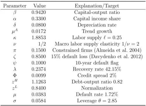
Table 2: Parameters (Steady State) Parameter Value Explanation/Target

β 0.9420 Capital-output ratio

α 0.3300 Capital income share

δ 0.0800 Depreciation rate

µA _{0.0172 Trend growth}

κ 1.8853 Labor supply `= 0.25

ν 1/2 Macro labor supply elasticity 1/ν = 2

π 0.1500 Constrained firms (Almeida et al. 2004)

ζ 0.8500 15% default loss (Davydenko et al. 2012)

ψ 0.1000 10-year default flag

λ 0.2374 Recovery rate 42.15% Φ 0.0099 Credit spread 2% zH 1.1263 Debt-output ratio 0.82 zL _{0.8400 Normalization} µ 0.0383 Default rate 1.72% σ 0.0584 Leverageθ = 2.85

Directly calibrated are 1− α = 0.67 (labor share), δ = 0.08 (annual depreciation rate),

µA = 0.0172 (growth rate of per capita output), 1 − ζ = 0.15 (direct net-worth losses in default, see Davydenko et al. (2012)), and ψ = 0.1 which implies a ten-year exclusion period.18

According to Fiorito and Zanella (2012) and Keane and Rogerson (2012), the macro labor supply elasticity that allows for both intensive and extensive margin adjustments should be 1.5–2, so we set the labor supply elasticity to 1/ν = 2. We then setκ = 1.8853 by arbitrarily normalizing steady-state labor supply at 0.25. We set probabilityπ= 0.15 so that 15 percent of firms are financially constrained (Almeida et al. (2004)), Kaplan and Zingales (1997)).

We normalize average capital productivity at ˜z =πzH_{+ (1−π)z}L_{+f πθ(z}H_−zL_{) = 1.}19 The normalization pins down zH_{, given parameters π, z}L_{, the debt-to-equity ratio θ, and} the steady-state value of the fraction of firms with credit market access f.

The remaining six parameters are calibrated jointly to match the following targets: (i) the capital-output ratio K/Y = 2; (ii) the credit-output ratio B/Y = 0.82, based on all (non-financial) firm credit 1982–2015; (iii) the leverage ratio θ = 2.85 in credit-constrained

18_{This corresponds to the bankruptcy flag for sole proprietors (or for partnerships with personal liabilities)}

filing for bankruptcy under Chapter 7 of the U.S. Bankruptcy Code.

19_{Without this normalization,δ would not be the depreciation rate of this economy: (1−δ)˜zK}

t of the

capital stock survives to the next period. Hence, depreciation isKt−(1−δ)˜zKt, and the depreciation rate

firms;20 _{(iv) a recovery rate of 42.15%; (v) a 1.72% default rate; (vi) a 2% credit spread (see} Section 2). These targets identify the six parametersβ, µ, σ, γ =zL_/zH_{,λ and Φ uniquely.} The discount factor β determines the investment rate and the capital-output ratio. The average default cost µ determines the default rate. The recovery parameter λ is identified from the recovery rate, and Φ is calibrated to match the excess bond premium (i.e. the fraction of the spread not accounted for by expected default losses). The remaining two parameters, the variance of default costs σ and the productivity ratio γ, are determined from average credit and the leverage ratio of constrained firms. For details how we calculate these parameters from the calibration targets, see Appendix B. All parameter values are shown in Table 2.

We linearize the system around the deterministic steady state. We then explore the equilibrium dynamics in response to all three financial shocks (spread shocks, collateral shocks, and sunspots) together with productivity shocks. That is, besides estimating the shocks to µA

t , we estimate shocks to the recovery parameter λt, intermediation cost Φt, and sunspots εt.

We use the time series data for the recovery rate, default rate, spreads, and output growth described in Section 2. We use the maximum likelihood method and estimate AR(1) processes for Φt,µA_t, λt and finally the sunspot εt which satisfy

log(1 + Φt)−log(1 + Φ) =ρΦ[log(1 + Φt−1)−log(1 + Φ)] +ξtΦ , log(1 +µA_t )−log(1 +µA) = ρA

log 1 +µA_t−1−log 1 +µA+ξ_tA ,

log(1 +λt)−log(1 +λ) = ρλ[log (1 +λt−1)−log (1 +λ)] +hΦλξ Φ t +h A λξ A t +ξ λ t , εt=hΦεξtΦ+hAεξtA+hλεξλt +ξtε ,

whereρΦ,ρA, andρλ are persistence parameters, andξtΦ,ξtA,ξλt andξεt are i.i.d. normally dis-tributed with mean zero and variancesσ2

Φ,σA2,σλ2 andσε2. These random variables are called below “intermediation shocks”, “productivity shocks”, “collateral shocks”, and “sunspot shocks”, respectively. Collateral shocks and sunspot shocks are essentially “credit demand” shocks, while intermediation shocks affect the banks’ willingness to supply credit.

The idea behind this structure is as follows.21 _{Following Gilchrist and Zakrajˇsek (2012),} who find that “excess bond premium” can lead many important financial variables, we allow intermediation shocks to also affect the recovery parameter λt as well as changes in credit market expectationsεt. In addition, we allow aggregate productivity shocks to affectλt and 20_{This corresponds to the 85th percentile of debt-equity ratios of firms in the Survey of Small Business}

Finances 2003 (Federal Reserve Board) and to the 90th percentile in Compustat.

21_{We experimented with different specifications, such as setting the impact of productivity shocks on}

εt as well, in order to capture unmodelled linkages between the real economy and financial markets. Further, we allow changes in the recovery ability to also take an impact on the sunspot variableεt. Next to the impact of fundamental shocks on credit market expectations, reflected in parameters hΦ

ε, hAε and hλε, there are also sunspot shocks ξtε that directly affect the sunspot state εt.

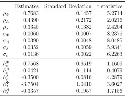
Table 3 presents the estimation results. Intermediation shocks seem to generate the most persistent effects (ρΦ is the largest among persistent parameters). The estimates of all standard deviations of the shocks are highly significant, implying that all four shocks are indeed important to capture different aspects of the business cycle.

Table 3: Estimation Results

Estimates Standard Deviation t statistics

ρΦ 0.7683 0.1457 5.2714 ρA 0.4390 0.2172 2.0216 ρλ 0.3345 0.1382 2.4204 σΦ 0.0060 0.0007 8.2375 σA 0.0390 0.0048 8.0485 σλ 0.0352 0.0059 5.9341 σε 0.0136 0.0022 6.2263 hΦ ε 0.7568 0.6519 1.1609 hA_ε -0.0421 0.1114 0.4079 hλ ε -0.3500 0.0816 4.2879 hΦ λ -3.7504 1.0410 3.6027 hA_λ -0.3357 0.1957 1.7156

Notice that the standard deviation of collateral shocks is almost six times of that of intermediation shocks, while|hΦ

ε|is only about twice as large as|hλε|. This comparison means that the spill-over effect of intermediation shocks on sunspots is much weaker compared to the one of collateral shocks on sunspots. Additionally, the effect of intermediation shocks on sunspots is not significantly different from zero either. Using the same logic, we find that the effect of productivity on sunspots is neither large nor significant.

Finally, when we look at spill-over effects on the recovery parameter λt, either from intermediation shocks or from productivity shocks, it seems that the impact of intermediation shocks is more important. This result is intuitive. High excess bond premia may reflect a situation where assets cannot be easily liquidated so that the recovery of defaulted corporate bonds is lower.

5.2

Quantitative Results

Three sets of results are shown in the following. First, we show the smoothed shocks from the maximum likelihood estimation exercise. Second, we illustrate the impulses responses after one standard deviation for each of the shocks. Third, we show the variance decomposition into the four independent shocks, and we illustrate the contribution of the credit market ex-pectations channel for macroeconomic volatility. Finally, we compare the estimated sunspot series with a measure of expected credit market condition from survey data, which we argue provides some support for our theory.

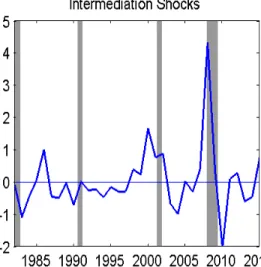
Estimated Shocks

All four estimated shocks are plotted in Figure 3, normalized by their standard deviations. Through the lens of our model, the 2007-2009 recession is indeed special compared to the previous ones. It has a combination of a fall in recovery ability, deteriorated credit market expectations (positive sunspot shocks), and the recession is led by a larger-than-usual inter-mediation cost shock. Aggregate productivity shocks do not show a clear pattern but are negative in 2007 and 2009.

The Great Recession featured a large liquidity and pledgeability drop of financial assets, which is captured in our model by the negative shocks to the collateral valueλ. Note also the positive shocks toλin the years prior to the Great Recession, which may reflect the real-estate boom and the surge of collateral assets in this period. After the recession, innovations to λ

become positive but then stay almost at zero, possibly due to the asset-purchase programs implemented by the Federal Reserve in 2009-2010.

The rise of shocks to intermediation costs in 2007 and 2008 reflects the sharp increase of the “excess bond premium” induced by the banking crisis at the onset of the financial crisis. Notice also the sharp fall of shocks to Φt in 2009 and 2010. Again, we can interpret this result as a consequence of government intervention in asset markets which may have significantly reduced risk aversion and other factors such as liquidity risks, contributing to the fall in bond premia.

We can observe a deterioration of credit market expectations (positive sunspot shocks) prior to all three recessions since 1982.22 As will become clear in impulse responses, sunspot shocks are quantitatively important for the business cycle, since they can move leverage significantly and thus affect output growth.

22_{Interestingly, the credit spread did not increase during the 1991 recession, despite a significant increase}

Figure 3: Estimated Shocks. Note: All shocks are normalized by their respective standard deviations. Shaded areas are NBER dated recessions.

Impulse Responses

To gain intuition for the role of the four independent shocks, we illustrate the transmission mechanisms by impulse response functions. We plot these functions for various variables of interest. In all cases, the economy starts from steady state and is hit by one standard deviation of a particular shock at time zero.

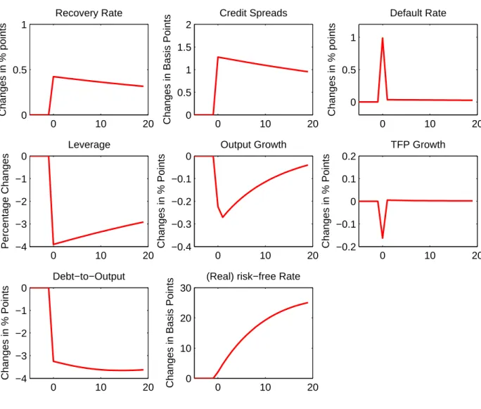
We first describe the impact of shocks to credit market expectations. Figure 4 shows the impulse response functions when a one-time sunspot shock hits the economy. The shock raises the default rate on impact by one percentage point after which default falls back but remains persistently slightly above the steady-state level. An important consequence of

Figure 4: Impulse Responses for a One Time Sunspot Shock 0 10 20 0 0.5 1 Changes in % points Recovery Rate 0 10 20 0 0.5 1 1.5 2

Changes in Basis Points

Credit Spreads 0 10 20 0 0.5 1 Changes in % points Default Rate 0 10 20 −4 −3 −2 −1 0 Percentage Changes Leverage 0 10 20 −0.4 −0.3 −0.2 −0.1 0 Changes in % Points Output Growth 0 10 20 −0.2 −0.1 0 0.1 0.2 Changes in % Points TFP Growth 0 10 20 −4 −3 −2 −1 0 Changes in % Points Debt−to−Output 0 10 20 0 10 20 30

Changes in Basis Points

(Real) risk−free Rate

sunspot shocks is that the leverage ratio falls persistently, because credit market valuations (default incentives) remain persistently low (high) from time zero onward. Lenders, who take these incentives into account, tighten the credit constraints and charge (slightly) higher interest rates.23 _{After the sunspot shock, the persistent response of all variables is the key} to sustain a self-fulfilling credit cycle. In fact, if the deterioration of credit conditions was rather short-lived, the value of credit market access does not fall much, which implies that default rates can go up only little today. That is, sizable responses of default rates require a persistent credit market response.

Productive firms as borrowers are hurt by this disturbance in the credit market. Because 23_{Since the leverage ratio is much lower than the steady-state level, the recovery rate per unit of lending}

rises. Through tightening credit constraints, lenders are able to recover a greater share of their exposure after a default.

of the fall of leverage, these firms use a smaller share of the aggregate capital stock which dampens aggregate productivity. Therefore, we observe an endogenous fall of TFP which results in a 0.22 percentage-point reduction of the output growth rate, followed by another reduction of 0.28 percentage points in the next year. The real interest rate rises because of the rise of the profit rate Π in order to induce low-productivity firms to save in the capital market. The profit rate goes up because of the fall in aggregate labor demand which reduces the wage rate below the steady-state level.

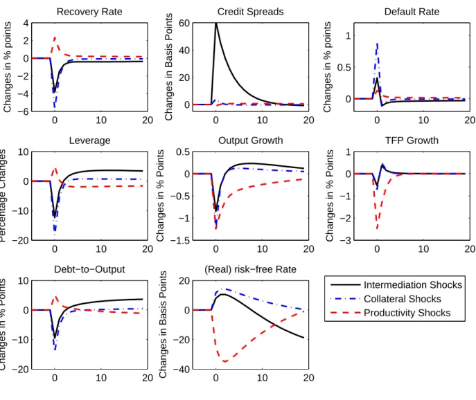
By comparison, we plot impulse response functions after all three fundamental shocks in Figure 5. A one standard-deviation (negative) collateral shock lowers the collateral value, so that lenders tighten credit on impact and charge a (slightly) higher interest rates to com-pensate for the losses. But the fall in leverage only lasts for two years, as the autocorrelation of λ is rather small. Since the fall in collateral value also raises the sunspot εt, we see a 0.8 percentage-point spike of the default rate. In expecting higher leverage in the future, firms have less incentive to default, and this is why the default rate falls (about -0.1 percentage points below the steady-state value) immediately after the initial rise.

In response to a rise in intermediation costs, the credit spread increases significantly (60 basis points) and it raises the default rate (0.35 percentage points). Since the rise of credit spreads further reduces the recovery parameter, leverage and output dynamics are similar to those after a collateral shock. One should notice that the credit-market response of the intermediation shock is mostly driven by the impact of the shock on the recovery parameter λt and on the sunspot εt. Consistent with Gilchrist and Zakrajˇsek (2012), the credit-spread shock induces a (rather short-lived) fall of output growth, while the default rate barely moves. This is because the modest fall of leverage offsets the negative impact on default incentives.

Finally, a negative productivity shock generates a persistent fall of output growth, partly because the process of productivity is persistent, but also because it slightly pushes up the sunspot εt. Recall that a sunspot shock persistently reduces output growth, as shown in Figure 4 and it induces a rise of the recovery rate. Compared to a pure sunspot shock, aggregate productivity reduces output directly, and this is why we see a rise of leverage and of the debt-to-output ratio after the initial productivity shock. Together with the fall of productivity, the risk-free rate falls since the profit rate Πt goes down.

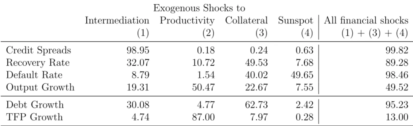
Variance Decomposition

Next we look at how much the variation in the data can be separately explained by the three financial shocks and aggregate productivity shocks. Then, we illustrate the channels through which these shocks operate: self-fulfilling credit market expectations, on the one

Figure 5: Impulse Responses after Adverse Fundamental Shocks 0 10 20 −6 −4 −2 0 2 4 Changes in % points Recovery Rate 0 10 20 0 20 40 60

Changes in Basis Points

Credit Spreads 0 10 20 0 0.5 1 Changes in % points Default Rate 0 10 20 −20 −10 0 10 Percentage Changes Leverage 0 10 20 −1.5 −1 −0.5 0 0.5 Changes in % Points Output Growth 0 10 20 −3 −2 −1 0 1 Changes in % Points TFP Growth 0 10 20 −20 −10 0 10 Changes in % Points Debt−to−Output 0 10 20 −40 −20 0 20

Changes in Basis Points

(Real) risk−free Rate

Intermediation Shocks Collateral Shocks Productivity Shocks

hand, or fundamental variables, on the other hand. This exercise is non-trivial because all fundamental shocks affect fundamental variables and credit-market expectations at the same time.

Evidently, from Table 4 the dynamics of recovery rates is mainly explained by collateral shocks (49.53%) and intermediation shocks (32.07%). Collateral shocks directly affect the recovery ability, while intermediation shocks affect both spreads and the recovery ability. The variations of default rates are mainly explained by financial shocks, including direct sunspot shocks (49.65%), collateral shocks (40.02%), and intermediation shocks (8.79%). Credit spread fluctuations are mostly explained by intermediation shocks which take a direct impact on spreads. It follows from our model that shocks to aggregate productivity do not play an important role for spreads, default rates and recovery rates. The VAR results of Section 2 suggest that this is a reasonable approximation.

Table 4: Variance Decomposition in Percents Exogenous Shocks to

Intermediation Productivity Collateral Sunspot All financial shocks

(1) (2) (3) (4) (1) + (3) + (4) Credit Spreads 98.95 0.18 0.24 0.63 99.82 Recovery Rate 32.07 10.72 49.53 7.68 89.28 Default Rate 8.79 1.54 40.02 49.65 98.46 Output Growth 19.31 50.47 22.67 7.55 49.52 Debt Growth 30.08 4.77 62.73 2.42 95.23 TFP Growth 4.74 87.00 7.97 0.28 13.00

Regarding output growth, sunspot shocks can explain 7.6% of the variation, while in-termediation shocks and collateral shocks explain 19.31% and 22.67%. Financial shocks together contribute to almost 50% of output variations because they affect the credit flow to productive firms.

There are two ways how the credit flow impacts output dynamics. On the one hand, the credit flow affects the capital allocation among productive and unproductive firms. This is the productivity effect of credit. On the other hand, the credit flow also affects the firms’ aggregate demand for capital and labor, and therefore aggregate production. This is the factor effect of the credit flow.

To shed light on these two effects, we show how the variation of debt growth and TFP growth in the model can be explained by each shock in the last two rows of Table 4. En-dogenous fluctuation of productivity growth due to the credit allocation is about 13%, which is much less important than the exogenous fluctuations in productivity growth (87%). Be-cause credit is mostly driven by financial shocks, credit does not generate large endogenous variation in TFP growth. Therefore, the main transmission mechanism of financial shocks is through the effect on the firms’ factor demands.

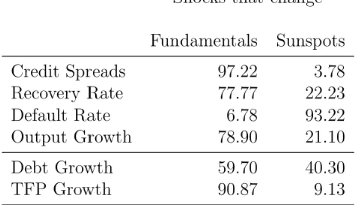
While the previous discussion focuses on the decomposition into exogenous shocks, we show now how these shocks impact credit market and macroeconomic variables through fundamental channels and the sunspot channel separately. This decomposition is impor-tant since we allow exogenous fundamental shocks (to collateral, intermediation costs or productivity) to affect the sunspot variable εt.

We use a simpleR-square statistics for this exercise. To see this, letξt= [ξΦt, ξtA, ξλt, ξtε]0be the collection of structural shocks. Then, the sunspot variable can be expressed asεt=cξt, where c= [hΦ_ε, hA_ε, hλ_ε,1]. If we are interested in, for example, the output growth gt, we run a population regression gt = βεεt+νt, where νt is orthogonal to εt. Then, the variation in

output growth explained by the sunspot channel can be expressed as the R-square of this regression.24 _{For other variables of interests, we simply repeat this procedure.}

Table 5: Variance Decomposition in Percents: Fundamentals versus Sunspots Shocks that change

Fundamentals Sunspots Credit Spreads 97.22 3.78 Recovery Rate 77.77 22.23 Default Rate 6.78 93.22 Output Growth 78.90 21.10 Debt Growth 59.70 40.30 TFP Growth 90.87 9.13

Table 5 shows that shocks that affect sunspots εt explain 21.1% of output growth vari-ations. The transmission mechanism can be seen again from a rather small effect on pro-ductivity growth (9.13% of TFP growth variation is explained by the sunspot channel), so that the sunspot channel operates mainly through factor demands. The sunspot channel is particularly important for the dynamics of default rates, and it also matters for variation of recovery rates, but it plays almost no role for fluctuations of credit spreads.

Some Supporting Evidence for Sunspots

As we have seen, the variation in default rates is mainly caused by changes in beliefs in credit market conditions, which affects the credit flow and aggregate real activity. We find some supporting evidence showing that our estimated sunspot variable is indeed closely linked with changes in expected credit market conditions.

There is a monthly survey conducted for small business firms which is called Small Busi-ness Economic Trends (SBET). It is a monthly assessment of the U.S. small-busiBusi-ness economy and its near-term prospects since January 1986. Its data are collected through mail surveys to random samples of the National Federal of Independent Business (NFIB) membership. NFIB is the largest small-business trade association in the country with members scattered across every state and every industry group. Despite the organization-based sampling frame, the SBET has been shown to be a reliable gauge of small business economic activity over the past decades, and its results regularly appear in mass media.

24_{That is,R}2₌ V ar(βε_ε t)

V ar(gt) , whereβ

ε₌ Cov(gt,εt)

V ar(εt) . Therefore, the variance ofgt explained by the sunspot

Figure 6: Sunspots and Credit Market Expectations. Note: Sunspots are estimated from the model. The original survey measure (from Small Business Economic Trends, SBET) is the percent of respondents who think that credit conditions will be “easier” minus those who think credit conditions will be “harder”. We multiply the original survey measure by -1 and plot the changes from the mean in standard deviations.

The survey contains a category called “expected credit conditions”, measured by the percent of respondents who think that credit conditions will be “easier” minus those who think credit conditions will be “harder”. When the measure falls, more respondents expect the credit condition to be tougher and therefore the excess value of credit market access should be lower.

We link the variation of this measure to the sunspots as identified by our model. The SBET report suggests that an important reason for borrowing is to pay wages in advance. For this reason, and to remove the more noisy responses of the smallest businesses, we focus on the sample of firms with at least 39 employees (which is the group of