P
RECISION
G
ATING
: I
MPROVING
N
EURAL
N
ETWORK
E
FFICIENCY WITH
D
YNAMIC
D
UAL
-P
RECISION
A
CTI
-VATIONS
Anonymous authorsPaper under double-blind review
A
BSTRACTWe propose precision gating (PG), an end-to-end trainabledual-precision quanti-zation technique for deep neural networks. PG computes most features in a low precision and only a small proportion of important features in a higher precision. Precision gating is very lightweight and widely applicable to many neural network architectures. Experimental results show that precision gating can greatly reduce the average bitwidth of computations in both CNNs and LSTMs with negligible accuracy loss. Compared to state-of-the-art counterparts, PG achieves the same or better accuracy with 2.4×less compute on ImageNet. Compared to 8-bit uni-form quantization, PG obtains a 1.2% improvement in perplexity per word with 2.8×computational cost reduction on LSTM on the Penn Tree Bank dataset. Pre-cision gating has the potential to greatly reduce the execution costs of DNNs on both commodity and dedicated hardware accelerators. We implement the sampled dense-dense matrix multiplication kernel in PG on CPU, which achieves up to 8.3×wall clock speedup over the dense baseline.
1
I
NTRODUCTIONIn recent years, deep neural networks (DNNs) have demonstrated excellent performance on many computer vision and language modeling tasks including image classification, semantic segmenta-tion, face recognisegmenta-tion, machine translation and image captioning (Krizhevsky et al., 2012; He et al., 2015; Ronneberger et al., 2015; Chen et al., 2016; Zhao et al., 2018; Schroff et al., 2015; Luong et al., 2015; Vaswani et al., 2017). One visible trend in DNN design is that as researchers strive for better accuracy, both the model size and the number of DNN layers have increased over time (Xu et al., 2018). At the same time, there is a growing demand to push deep learning technology to edge devices such as mobile phones, Internet of Things (IoT) devices, and lightweight drones (Wu et al., 2019). The limited computational, memory, and energy budgets on these devices create major challenges for the deployment of large DNN models on the edge.
Neural network quantization is an important technique for improving the hardware efficiency of DNN execution. Circuits operating at a lower precision are smaller, faster, and consume less energy. Numerous studies have shown that full-precision floating-point computation is not necessary for DNN inference — quantized fixed-point models produce competitive results with a small or zero loss in prediction accuracy (Lin et al., 2016; He et al., 2016; Zhou et al., 2016; 2017). In some cases, quantization may even improve model generalization by acting as a form of regularization. Existing studies mainly focus on static quantization, in which the precision of each weight and activation is fixed at run time (Hubara et al., 2017; He et al., 2016). Along this line of work, researchers have explored tuning the bitwidth per layer (Wu et al., 2018; Wang et al., 2018a; Dong et al., 2019) as well as various types of quantization functions (Wang et al., 2018b; Courbariaux et al., 2016; Li et al., 2016; Zhou et al., 2016). However, static DNN quantization methods cannot exploit input-dependent characteristics, where certain features during inference may contribute less to the classification result than others and can be computed in lower precision. For example, in computer vision tasks the pixels representing the object of interest are typically more important than the background pixels.
In this paper, we propose to reduce the inefficiency of a statically quantized DNN via precision gating(PG), which computes most features with low-precision arithmetic and only updates few
im-portant features to high precision. More concretely, PG first executes a DNN layer in low precision and identifies the output features with large magnitude as important features. It then computes a sparse update to increase the precision of those important output features. Intuitively, small values make very little contribution to the DNNs output; approximating them in low-precision is reason-able. Precision gating enables dual-precision DNN execution at the granularity of each individual output feature, and therefore greatly reducing the average bitwidth and computational cost of DNNs. To show the visualization of PG, we refer readers to Appendix A.1.
We further introduce a differentiable gating logic which makes the technique applicable to a greater variety of network models. Experimental results show that precision gating achieves significant speed-up and accuracy improvement on both CNNs and LSTMs. Compared to the baseline CNN counterparts, PG obtains 3.5% and 0.6% higher classification accuracy with up to 4.5×and 2.4×less computation cost for CIFAR10 and ImageNet, respectively. On LSTM, compared to 8-bit uniform quantization PG boosts perplexity per word (PPW) by 1.2% with 2.8×less compute on the Penn Tree Bank (PTB) dataset. Our contributions are as follows:
1. We propose precision gating, which to the best of our knowledge is the first end-to-end trainable method that enables dual-precision execution of DNNs. Precision gating is also applicable to a wide variety of network architectures (including both CNNs and RNNs). 2. Precision gating enables DNN computation with lower average bitwidth than other
state-of-the-art quantization methods. Combined with its lightweight gating logic, PG demonstrates the potential to reduce DNN execution costs in both commodity and dedicated hardware. 3. Unlike prior works that focus only on inference, precision gating achieves the same sparsity
during back-propagation as forward propagation, which dramatically reduces the compu-tational cost for both passes.
2
R
ELATEDW
ORKQuantizing activations. Prior studies show that weights can be quantized to low bitwidth without hurting much the accuracy (Zhu et al., 2017), but quantizing activations to low bitwidth typically incurs a large accuracy degradation. The problem is that large outliers in the activations make the quantization grid sparse under low precision, thus increasing the error. To address the problem, Choi et al. (2018) propose PACT to reduce the dynamic range of the activations through clipping the outliers by a learnable threshold, which provides a better quantization scheme for ultra low bitwidth. PACT is reported to be able to quantize activations to arbitrary bitwidth with better accuracy than other works. We incorporate PG with PACT to address the same large outlier problem. Moreover, PG is a dynamic quantization scheme whereas PACT is a static apporach.
Prediction-based execution. To lower the computation cost of a convolutional layer, some prior works explored the method of predicting ReLU-induced zeros or Max-pooling-induced compute redundancy in CNNs. For example, Lin et al. (2017); Song et al. (2018) proposezero-prediction to utilize a few most-significant bits in multipliers to identify the sign of the output elements. The rationale behind is that negative outputs will be suppressed by the ReLU anyway. The limitations of this method are that it only applies to ReLU activations and only when the ReLU must follow directly after the weight layer. As a result, the method cannot be applied to modern CNNs with a batch norm layer (Ioffe & Szegedy, 2015) before the ReLU or RNNs (which use sigmoid or tanh as the activation function). Cao et al. (2019) proposeSeerNetin which for each convolutional layer it first executes a duplicated quantized version of that layer to predict the output sparsity induced by the following ReLU or Max-pooling. It then computes the sparse original full-precision (32-bit floating-point) convolutional layer to obtain the outputs. Results of the quantized layer are not reused. Though the original layer is executed sparsely, practically the extra quantized layer induces higher execution cost.
Feature level precision tuning.There is also prior work that uses different precision at the feature level. Park et al. (2018) propose value-aware quantization where the majority of data are computed at reduced precision while a small number of outliers are handled at high precision. Our approach is significantly different because we apply dual precision for every feature, not only for the outliers. Hua et al. (2018) propose channel gating to dynamically turn off a subset of channels that contribute little to the classification result. Precision gating is orthogonal to this pruning technique as channel gating executes the whole network in the same precision.
1 0 1 1 0 0 1 1 1 0 1 1 0 0 1 1 Input Activations ℎ
=
ℎ<<
+
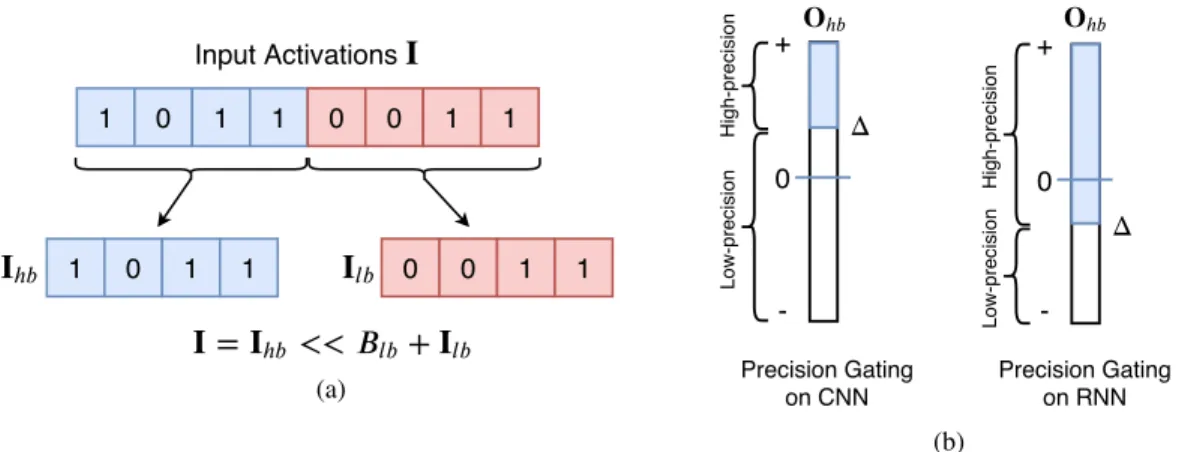
(a) 0 -+ ℎ ℎ High-precision Precision Gating on CNN Precision Gating on RNN 0 -+ High-precision Δ Δ Low-precision Low-precision (b)Figure 1:(a)Splitting an input featureIintoIhb, the most-significantBhbbits, andIlb, the remaining
Blbbits. The total bitwidth isB.(b)PG achieves savings by comparingOhbto some nonzero value
to do prediction.
3
P
RECISIONG
ATINGIn this section, we first describe the basic mechanism of precision gating. Then we discuss how to design the gating logic to accelerate both forward and backward passes. Finally, we incorporate PG with outlier clipping to reduce the quantization error.
3.1 BASICFORMULATION
Define a linear layer (i.e. convolutional or fully-connected layers) in a neural network asO=I∗W, whereO,I, andWare the output, input, and weights, respectively. LetIbe represented in aB-bit fixed-point format. As shown in Figure 1a, precision gating partitionsIintoIhb, the most-significant
Bhbbits, andIlb, the remainingBlbbits, whereB=Bhb+Blb. More formally, we can write:
I=Ihb<< Blb+Ilb (1)
Here<<is the shift operator. We can then reformulate a singleB-bit linear layer into two lower-precision computations as:
O=Ohb+Olb= [W∗(Ihb<< Blb)] + [W∗Ilb] (2)
Ohbis the partial sum obtained by using the MSBs of input feature (Ihb) whereasOlbrepresents the
remaining sum computed withIlb.
Precision gating works in two phases. In theprediction phase, precision gating performs the compu-tationOhb=W∗(Ihb<< Blb). Elements ofOhbgreater than a gating threshold∆are considered
important. In theupdate phase, precision gating computesOlb =W∗Ilbonly for the important
elements and adds it toOhb. Precision gating’s execution flow is shown in Figure 2: unimportant
output features take only the upper path while important ones are computed as the sum of both paths. Precision gating can be summarized as:
O=
Ohb Ohb≤∆
Ohb+Olb Ohb>∆ (3)
In essence, precision gating computes important features withB-bit arithmetic and unimportant fea-tures with onlyBhbbits. The importance of each element in the outputOis predicted by comparing
the magnitude of its partial sumOhbto∆. Letpbe the percentage of important activations over
all features. PG saves (1−p)·Blb
B fraction of the compute in the original DNN model. Figure 1b
illustrates which values are executed in high-precision. PG thus achieves dual-precision execution using a lightweight gating mechanism, and reduces theaverage bitwidthof computations in a DNN.
3.2 EFFICIENTLEARNABLEGATINGLOGIC
In order to automatically determine model and dataset specific threshold∆, we propose an efficient end-to-end trainable gating logic. The gating threshold∆is specific to each output channel in DNN
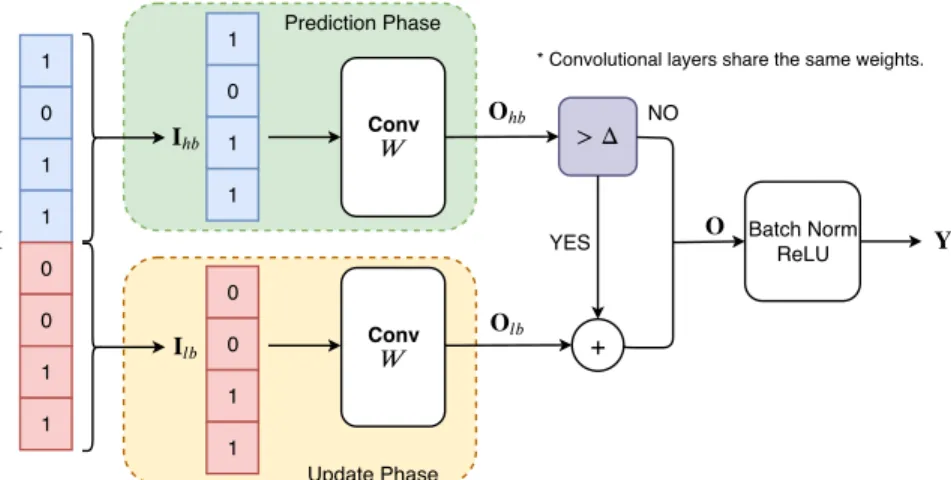
1 0 1 1 0 0 1 1 1 0 1 1 0 0 1 1 ℎ Conv > Δ ℎ +
YES Batch Norm
ReLU NO
Conv
* Convolutional layers share the same weights.
Prediction Phase
Update Phase
Figure 2: The PG building block in CNN models –Input features are split intoIhb andIlb. In
the prediction phase, Ihb first convolves with the full precision filters Wto obtainOhb. In the
update phase, if the partial sumOhbof a feature exceeds the learnable threshold∆, we will update
that feature to high-precision by addingOlbtoOhb. Otherwise, we skip the update phase, and the
output feature therefore remains computed at ultra low-precision.
layers and learned alongside the DNN weights during training. A larger∆indicates that more output features are computed in low-precision, resulting in greater computational savings but possibly at the expense of reduced model accuracy. We formulate the problem of optimizing∆as minimizing the original model lossLalong with an L2 penalty term:
min
W,∆L(I, y;W,∆) +σk∆−δk 2
(4) Hereyis the ground truth label,σis the penalty factor, andδis thegating target, a target value for the learnable threshold. The penalty factor and gating target are hyperparameters which allow a user to emphasize high computation savings (largeσorδ) or accuracy preservation (smallσorδ). Training a model with precision gating can be done on commodity GPUs using existing deep learn-ing frameworks. We implement PG on GPU as the equation O = Ohb +maskOlb, where
mask =1Ohb>∆ is a binary decision mask andrepresents element-wise multiplication. Dur-ing forward propagation, most elements inmaskare 0. PG therefore saves hardware execution cost by only computing a sparseOlbin the update phase. In dedicated hardware, MSBs and LSBs
are wired separately. The prediction phase is controlled by a multiplexer, and only computes LSB convolutions whileOhbexceeds the threshold, thus achieving the savings.
The mask is computed using a binary decision function (i.e. step function), which has a gradient of zero almost everywhere. To let gradients flow throughmaskto∆, we use a sigmoid on the backward pass to approximate the step. Specifically, we definemask = sigmoid(α(Ohb−∆))
only on the backward pass following Hua et al. (2018). Hereαchanges the slope of the sigmoid, thus controlling the magnitude of the gradients.
3.3 SPARSEBACK-PROPAGATION
A sparse update phase only reduces the computational cost during the inference (forward propa-gation). We further propose to save the compute during the back-propagation by modifying the forward function of the PG block. Specifically, we square themaskelement-wise.
O=Ohb+mask2Olb (5)
Given thatmaskis a binary tensor,mask2 in Eq. (5) preserves the same value asmask. Thus the forward pass remains unchanged. During the back-propagation, an additionalmaskterm is introduced in computing the gradient ofOwith respect to the gating threshold∆in Eq. (6) because of the element-wise square. Consequently, the update of∆only requires the result ofmaskOlb
which has already been computed during the forward pass.
∂O ∂∆ ≈ ∂O ∂mask ∂sigmoid(α(Ohb−∆)) ∂∆ = 2·maskOlb ∂sigmoid(α(Ohb−∆)) ∂∆ (6)
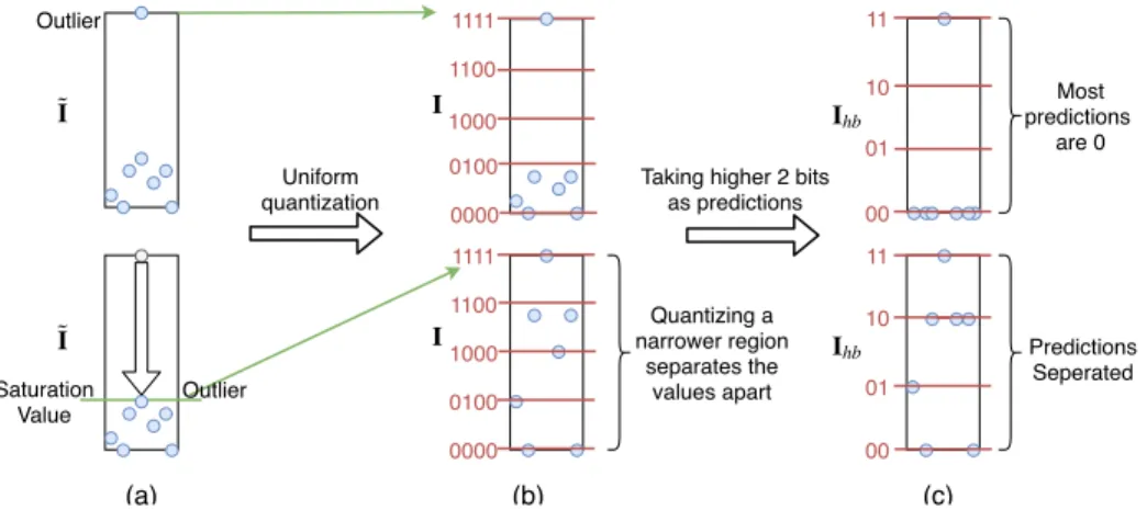
Predictions Seperated 00 11 11 00 01 10 Ihb Ihb Most predictions are 0 Saturation Value Ĩ Ĩ Outlier Outlier I 0000 0100 1111 0000 0100 1111 1000 1100
I narrower regionQuantizing a separates the
values apart
(a) (b) (c)
Uniform quantization
Taking higher 2 bits as predictions 1000
1100
10 01
Figure 3:Effect of clipping –A toy example illustrating how a clip threshold helps separating pre-diction values apart. The first row is quantization and prepre-diction without a clip threshold, while the second row has a clip threshold.(a)Distribution of floating-point input features˜I. (b)Distribution ofIafter quantizing˜Ito 4 bits.(c)Distribution ofIhbwhich takes the higher 2 bits ofI.
The gradient ofOwith respect to the weightsWin Eq. (7) employs the same sparsemaskOlb
as the update of∆. Therefore, precision gating can reduce the computational cost of both forward-progagtion (inference) and back-propagation by the same factor.
∂O ∂W = ∂Ohb ∂W +mask 2 ∂Olb ∂W = ∂Ohb ∂W + ∂maskOlb ∂W (7) 3.4 OUTLIERCLIPPING
Precision gating identifies important features using low-precision computation. One difficulty with this is that DNN activations are distributed in a bell curve, with most values close to zero and a few large outliers. The top row of Figure 3(a) shows some activations in blue dots, including a single outlier. If we quantize each value to 4 bits (second column) and use 2 most-significant bits in the prediction phase (third column), we see that almost all values are rounded to zero. In this case, PG can only distinguish the importance between the single outlier and the rest of the values no matter what∆is. Thus the presence of large outliers greatly reduces precision gating’s effectiveness. To address this, we combine precision gating with PACT (Choi et al., 2018), which clips each layer’s outputs using a learnable clip threshold. The bottom row of Figure 3 shows how clipping limits the dynamic range of activations, making values more uniformly distributed along the quantization grid. Now the 2 most-significant bits can effectively separate out different groups of values based on magnitude. We apply PACT to precision gating in CNNs, which typically use an unbounded activation function (ReLU). RNNs typically employ a bounded activation function (tanh, sigmoid), making PACT unnecessary.
4
E
XPERIMENTSWe test precision gating using ResNet-18 (He et al., 2015) and ShiftNet-20 (Wu et al., 2017) on CIFAR-10 (Krizhevsky & Hinton, 2009), and ShuffleNet V2 (Ma et al., 2018) on ImageNet (Deng et al., 2009). ResNet is a very popular CNN for image classification, and the other two lightweight architectures are designed specifically for edge devices. We set the expansion rate of ShiftNet to be six and choose the 0.5×variant of ShffleNet V2 for all experiments. On CIFAR-10, the batch size is 128, and the models are trained for 200 epochs. The initial learning rate is 0.1 and decayed at epoch 100, 150, 200 by a factor of 0.1 (multiply learning rate by 0.1). On ImageNet, the batch size is 512 and the models are trained for 120 epochs. The learning rate decayed linearly from an initial value of 0.5 to 0.
We also test an LSTM (Hochreiter & Schmidhuber, 1997) on the Penn Tree Bank (PTB) (Marcus et al., 1993) corpus. The model accuracy is measured by perplexity per word (PPW), and lower is
better. Following the configuration used by He et al. (2016) and Hubara et al. (2017), the number of hidden units in the LSTM cell is set to 300, and the number of layers is set to 1. We follow the same training setting as described in He et al. (2016), except the learning rate decayed by a factor of 0.1 at epoch 50 and 90. All experiments are run on Tensorflow (Abadi et al., 2016) with NVIDIA GeForce 1080Ti GPUs. We report the top-1 accuracy for all experiments.
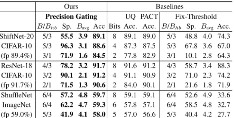
Table 1: Precision gating (PG) on CNN – models tested are ShiftNet-20 and ResNet-18 on CIFAR-10, and ShuffleNet V2 0.5×
on ImageNet. We compare PG against uniform quantization (UQ), PACT, and Fix-Threshold. Bavg is the average bitwidth (Bavg =
Bhb+ (1−Sp%)×(B−Bhb)). “fp” is floating-point. “Sp.” is
sparsity.
Ours Baselines
Precision Gating UQ PACT Fix-Threshold B/Bhb Sp. Bavg Acc Bits Acc. Acc. B/Bhb Sp. Bavg Acc. ShiftNet-20 5/3 55.5 3.9 89.1 8 89.1 89.0 5/3 48.8 4.0 74.3 CIFAR-10 5/3 96.3 3.1 88.6 4 87.3 87.5 5/3 67.8 3.6 67.0 (fp 89.4%) 3/1 71.9 1.6 84.5 2 77.8 82.9 3/1 10.1 2.8 64.3 ResNet-18 4/3 78.2 3.2 91.7 8 91.6 91.2 4/3 58.7 3.4 88.3 CIFAR-10 3/2 90.1 2.1 91.2 4 91.1 90.9 3/2 71.0 2.3 74.2 (fp 91.7%) 2/1 71.5 1.3 90.6 2 84.0 90.1 2/1 21.6 1.8 71.9 ShuffleNet 6/4 57.2 4.8 59.7 8 59.1 59.1 6/4 52.6 4.9 33.6 ImageNet 6/4 62.2 4.7 59.3 6 57.8 57.1 6/4 58.5 4.8 32.7 (fp 59.0%) 5/3 41.9 4.1 58.0 5 57.0 56.6 5/3 40.4 4.2 27.7
Table 2: Precision gating (PG) on CNN –compare PG against SeerNet under similar model prediction accuracy. In SeerNet the average bitwidth
Bavg=Bhb+ (1−Sp%)×B.
ShiftNet ResNet ShuffleNet
SeerNet B/Bhb 12/8 6/4 8/6 Sp. 49.7 51.1 30.8 Bavg 14.0 6.9 11.5 Acc. 85.4 91.2 58.9 PG B/Bhb 5/3 3/2 6/4 Sp. 96.3 90.1 62.2 Bavg 3.1 2.1 4.7 Acc. 88.6 91.2 59.3
We replace the conv layers in CNNs and FC layers in LSTM with the proposed PG block. Moreover, the following hyperparameters in PG need to be tuned appropriately to achieve low average bitwidth with high accuracy.
• The full bitwidthB –this represents the bitwidth for high-precision computation in PG.
Bis set to 5 or less on CIFAR-10, 5 or 6 on ImageNet, and 3 or 4 on PTB.
• The prediction bitwidthBhb–this represents the bitwidth for low-precision computation.
• The penalty factorσ–this is the scaling factor of the L2 loss for gating thresholds∆.
• The gating targetδ–the target gating threshold. We use a variety of valuesδ∈[−1.0,5.0] in our experiments.
• The coefficientαin the backward pass –αcontrols the magnitude of gradients flowing to∆. We setαto be 5 across all experiments.
4.1 CNN RESULTS
To compare hardware execution efficiency across different techniques, we compute theaverage bitwidth(Bavg) of all features in a DNN model:
Bavg=Bhb+p∗Blb (8)
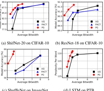
wherepis the percentage of high-precision activations (i.e. number of important features divided by total features). The computational cost of DNNs is proportional to the average bitwidth. Our results on CNNs are presented in Table 1 and Table 2, where sp. stands for sparsity.
We first compare PG against two widely adopted quantization schemes — uniform quantization (UQ) and PACT (Choi et al., 2018). In Table 1, the 3rd and 4th columns show the average bitwidth and model accuracy of PG whereas the 5th–8th columns list the bitwidth and corresponding model accuracy of UQ and PACT. At each row PG achieves better accuracy with fewer average bitwidth (Bits vs. Bavg). Specifically, PG achieves6.7%and1.6%higher accuracy with1.25×
computa-tional cost reduction , and6.6%and0.5%higher accuracy with1.54×computational cost reduction than 2-bit UQ and PACT on ShiftNet-20 and ResNet-18 for CIFAR-10 (3rd & 6th rows), respec-tively. We observe the same trend on ShuffleNet for ImageNet where PG improves the accuracy of 5-bit UQ and PACT by1.0%and1.4%with1.22×computational cost reduction (9th row). It is also worth noting that PG can recover the accuracy of the floating-point ShiftNet-20, ResNet-18,
and ShuffleNet with3.9,3.2, and4.7average bitwidth. This demonstrates that PG, using a learnable threshold, can identify unimportant features and reduce bitwidth without compromising accuracy. We then compare PG with Fix-Threshold, which is an extension of zero-prediction (Lin et al., 2017; Song et al., 2018). Lin et al. (2017) and Song et al. (2018) explicitly predict ReLU-induced zeros during inference. To have a fair comparison, we extend their technique to predict an arbitrary fixed threshold to achieve the same or fewer Bavg as PG, reported as Fix-Threshold in Table 1. For CIFAR-10, we observe that PG achieves20.2%and18.7%higher accuracy with1.75×and1.38×
computational cost reduction than Fix-Threshold on ShiftNet-20 and ResNet-18 (3rd & 6th rows), respectively. The gap in accuracy becomes even larger on ShuffleNet V2 for ImageNet dataset. With the same or lower average bitwidth, the accuracy of PG is at least26%higher than Fix-Threshold. In conclusion, PG consistently outperforms Fix-Threshold at any bitwidth across all networks and datasets (7th – 9th rows). The reason is that PG learns to adjust the gating thresholds to the clipped activation distribution so that it predicts with less zero bits.
Table 3: PG with and without sparse back-propagation (SpBP) on CNNs
PG PG w/ SpBP
Bavg Sp. Bavg Sp. B/Bhb Acc
ShiftNet 4.0 49.3 3.9 55.5(↑6.2) 5/3 89.1 3.3 84.0 3.1 96.3(↑12.3) 5/3 88.6 ResNet 3.4 58.2 3.2 78.2(↑20.0) 4/3 91.7 2.2 76.5 2.1 90.1(↑13.6) 3/2 91.2 ShuffleNet 5.3 36.6 4.8 57.2(↑20.6) 6/4 59.7 5.1 43.1 4.7 62.2(↑19.1) 6/4 59.3
Table 4: PG on LSTM –the dataset used is Penn Tree Bank (PTB). The metric is perplexity per word (PPW) and lower is better. Floating-point PPW is 110.1. Base PG Bits PPW B/Bhb Sp. Bavg PPW 8 109.8 4/2 48.4 3.0 108.5 4 110.8 4/2 54.9 2.9 109.3 2 124.9 3/1 53.0 1.9 118.8 2 4 6 8 Average Bitwidth 77.5 80.0 82.5 85.0 87.5 90.0 Model Accuracy (%) UQ PACT PG
(a) ShifNet-20 on CIFAR-10
2 4 6 8 Average Bitwidth 89.0 89.5 90.0 90.5 91.0 91.5 92.0 Model Accuracy (%) UQ PACT PG (b) ResNet-18 on CIFAR-10 4 5Average Bitwidth6 7 8 9 56 57 58 59 60 Model Accuracy (%) UQ PACT PG (c) ShuffleNet on ImageNet 2 Average Bitwidth4 6 8 110 115 120 125
Perplexity Per Word UQPG
(d) LSTM on PTB
Figure 4: Precision gating (PG) results on CNNs and LSTM –compare PG against uniform quantization (UQ) and PACT.
We further compare PG with SeerNet (Cao et al., 2019) in Table 2. SeerNet adds an extra quantized conv layer to predict a sparse mask for executing the original floating-point layer during inference. As the code of SeerNet is unavailable, we implement the network in Tensorflow by ourselves and boost its accuracy by retraining the network. We reduce the average bitwidth of SeerNet while keep-ing a comparable accuracy as PG. At similar model prediction accuracy, PG achieves3.5%higher accuracy with3.3×and4.5×less compute on ResNet-18 and ShiftNet for CIFAR-10, respectively. For ImageNet, PG on ShuffleNet also achieves0.4%higher accuracy with2.4×computational cost reduction than SeerNet. PG outpeforms SeerNet as SeerNet uses the extra quantized layer for pre-diction only and its outputs are sparse thus inaccurate, while PG reuses the low-precision results and passes them to outputs anyway.
To quantify the impact of sparse back-propagation described in Section 3.3, we run PG with and without sparse back-propagation on CNNs. Table 3 compares the sparsity in the update phase of PG with and without back-propagation under the same model accuracy and average bitwidth. Surpris-ingly, we find that the sparsity in the update phase of PG with sparse back-propagation is consis-tently higher than that of PG without sparse back-propagation across all models and datasets. For both CIFAR-10 and ImageNet, the sparsity increment is between 6% and 21%. We hypothesize that sparse back-propagation zeros out the gradients flowing to non-activated LSB convolutions in the update phase, which leads to higher sparsity.
Overall, compared to other prediction based quantization schemes, our method has measurably up to 21.6% higher accuracy than the baseline with lower computational cost or up to 4.5×less compute
with the same or better accuracy for CIFAR-10. For ImageNet ours has a maximum of 30.3% higher accuracy with similar computational cost or 2.4×less computational cost with 0.4% higher accuracy. The results compared to quantization baselines are visualized in Figure 4, which plots accuracy vs. average bitwidth — uniform quantization (squares), PACT (triangles), and PG (circles) are shown on separate curves. Results closer to the upper-left corner are better.
4.2 LSTM RESULTS
Besides CNNs, PG works great on RNNs as well. The results on LSTM with PG for the PTB corpus are reported in Table 4. Here, only the uniform quantization is used as the baseline because PACT, Fix-Threshold, and SeerNet do not work for sigmoid or tanh activation functions. Although Hubara et al. (2017) claim that quantizing both weights and activations to 4 bits does not lower PPW, we observe a significant PPW degradation asBdecreases from 8 to 4 bits in our implementation. The LSTM with 8-bit activations is therefore considered as the full accuracy model. We observe the same phenomena as in the CNN results that PG enables the 3-bit LSTM cell to improve the PPW by 1.2%and reduce the computational cost by2.7×compared to 8-bit uniform quantization.
4.3 KERNELSPEEDUP
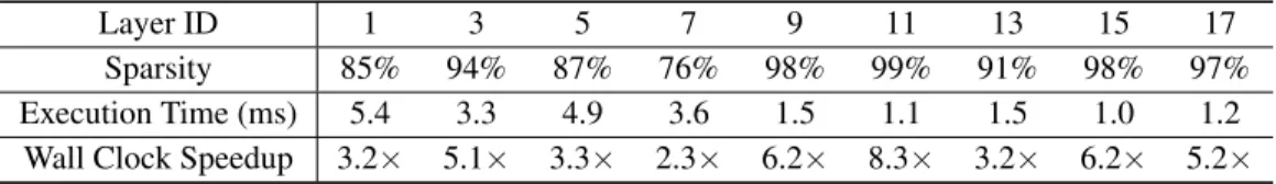
The sparse update phase of PG can be implemented efficiently with a new kernel called sampled dense-dense matrix multiplication (SDDMM). A convolutional layer with PG is then factorized into a regular low-precision convolution bounded with a low-precision SDDMM. To evaluate the actual speedup of PG, we implement the SDDMM kernel in Python leveraging a high performance JIT compiler Numba (Lam et al., 2015) and test it on the ResNet-18 model for CIFAR-10. Table 6 shows the layer-wise sparsity and the kernel speedup compared to the dense baseline on Intel Xeon Silver 4114 CPU (2.20GHz). With the large sparsity (from 76% to 99%) in each layer induced by PG, the SDDMM kernel achieves up to 8.3×wall clock speedup over the general dense matrix-matrix multiplication (GEMM) kernel. The significant wall clock speedup shows an enormous potential of deploying PG on commodity hardware.
Table 6:SDDMM kernel sparsity and speedup –We report optimized kernel execution time and wall-clock speedup of each layer in ResNet-18 for CIFAR-10.
Layer ID 1 3 5 7 9 11 13 15 17
Sparsity 85% 94% 87% 76% 98% 99% 91% 98% 97%
Execution Time (ms) 5.4 3.3 4.9 3.6 1.5 1.1 1.5 1.0 1.2
Wall Clock Speedup 3.2× 5.1× 3.3× 2.3× 6.2× 8.3× 3.2× 6.2× 5.2×
For a GPU implementation, we face the challenge in replacing the GEMM kernel with SDDMM kernel. Popular deep learning framework such as Tensorflow does not incorporate SDDMM as an built-in operator. However, Nisa et al. (2018) demonstrate that a highly optimized SDDMM kernel with a similar sparsity shown in Table 6 achieves about 4×speedup over a GEMM kernel. This shows strong evidence that PG has a potential to obtain high speedup on GPUs as well. Additionally, our approach is compatible with the specialized accelerator architectures proposed by Lin et al. (2017) and Song et al. (2018). Due to the enormous sparsity, DNNs with PG are estimated to get at least 3×speedup and 5×energy efficiency on these dedicated hardware accelerators. We leave the deployment of the SDDMM kernel on GPU and dedicated hardware to future work.
5
C
ONCLUSIONSWe propose precision gating, a dynamic dual-precision quantization method that can reduce the computation and storage costs of DNNs. PG assigns higher precision to important features and lower precision to the remaining features at run-time. The technique is end-to-end trainable allowing individual models to learn to distinguish salient and non-salient features. Experimental results show that PG outperforms state-of-the-art quantization and prediction approaches by a large margin on both CNN and RNN benchmarks on datasets such as Imagenet and Penn Tree Bank.
R
EFERENCESMart´ın Abadi, Paul Barham, Jianmin Chen, Zhifeng Chen, Andy Davis, Jeffrey Dean, Matthieu Devin, Sanjay Ghemawat, Geoffrey Irving, Michael Isard, Manjunath Kudlur, Josh Levenberg, Rajat Monga, Sherry Moore, Derek G. Murray, Benoit Steiner, Paul Tucker, Vijay Vasudevan, Pete Warden, Martin Wicke, Yuan Yu, and Xiaoqiang Zheng. Tensorflow: A system for large-scale machine learning. Proceedings of the 12th USENIX Conference on Operating Systems Design and Implementation, pp. 265–283, 2016. URLhttp://dl.acm.org/citation. cfm?id=3026877.3026899.
Shijie Cao, Lingxiao Ma, Wencong Xiao, Chen Zhang, Yunxin Liu, Lintao Zhang, Lanshu Nie, and Zhi Yang. Seernet: Predicting convolutional neural network feature-map sparsity through low-bit quantization.Conf. on Computer Vision and Pattern Recognition (CVPR), June 2019.
Liang-Chieh Chen, George Papandreou, Iasonas Kokkinos, Kevin Murphy, and Alan L. Yuille. DeepLab: Semantic Image Segmentation with Deep Convolutional Nets, Atrous Convolution, and Fully Connected CRFs.arXiv e-print, arXiv:1606.00915, Jun 2016.
Jungwook Choi, Zhuo Wang, Swagath Venkataramani, Pierce I-Jen Chuang, Vijayalakshmi Srini-vasan, and Kailash Gopalakrishnan. PACT: Parameterized Clipping Activation for Quantized Neural Networks.arXiv e-print, arXiv:1805.0608, 2018.
Matthieu Courbariaux, Itay Hubara, Daniel Soudry, Ran El-Yaniv, and Yoshua Bengio. Binarized Neural Networks: Training Deep Neural Networks with Weights and Activations Constrained to +1 or -1.arXiv e-print, arXiv:1602.02830, Feb 2016.
Jia Deng, Wei Dong, Richard Socher, Li-Jia Li, Kai Li, and Li Fei-Fei. ImageNet: A Large-Scale Hierarchical Image Database. Conf. on Computer Vision and Pattern Recognition (CVPR), pp. 248–255, 2009.
Zhen Dong, Zhewei Yao, Amir Gholami, Michael Mahoney, and Kurt Keutzer. HAWQ: Hessian AWare Quantization of Neural Networks with Mixed-Precision.arXiv e-print, arXiv:1905.03696, Apr 2019.
Kaiming He, Xiangyu Zhang, Shaoqing Ren, and Jian Sun. Deep Residual Learning for Image Recognition.arXiv e-print, arXiv:1512.0338, Dec 2015.
Qinyao He, He Wen, Shuchang Zhou, Yuxin Wu, Cong Yao, Xinyu Zhou, and Yuheng Zou. Effective Quantization Methods for Recurrent Neural Networks. arXiv e-print, arXiv:1611.10176, Nov 2016.
Sepp Hochreiter and Jrgen Schmidhuber. Long Short-Term Memory.Neural Computation, 9:1735– 80, Dec 1997. doi: 10.1162/neco.1997.9.8.1735.
Weizhe Hua, Christopher De Sa, Zhiru Zhang, and G. Edward Suh. Channel Gating Neural Net-works.arXiv e-print, arXiv:1805.12549, May 2018.
Itay Hubara, Matthieu Courbariaux, Daniel Soudry, Ran El-Yaniv, and Yoshua Bengio. Quantized Neural Networks: Training Neural Networks with Low Precision Weights and Activations. Jour-nal of Machine Learning Research (JMLR), 18(187):1–30, 2017.
Sergey Ioffe and Christian Szegedy. Batch Normalization: Accelerating Deep Network Training by Reducing Internal Covariate Shift. arXiv e-print, arXiv:1502.03167, Feb 2015.
Alex Krizhevsky and Geoffrey Hinton. Learning Multiple Layers of Features from Tiny Images. Tech report, 2009.
Alex Krizhevsky, Ilya Sutskever, and Geoffrey E Hinton. Imagenet Classification with Deep Con-volutional Neural Networks.Advances in Neural Information Processing Systems (NeurIPS), pp. 1097–1105, 2012.
Siu Kwan Lam, Antoine Pitrou, and Stanley Seibert. Numba: A llvm-based python jit compiler. Proceedings of the Second Workshop on the LLVM Compiler Infrastructure in HPC, pp. 7:1–7:6, 2015. doi: 10.1145/2833157.2833162.
Fengfu Li, Bo Zhang, and Bin Liu. Ternary Weight Networks. arXiv e-print, arXiv:1605.04711, May 2016.
Darryl D. Lin, Sachin S. Talathi, and V. Sreekanth Annapureddy. Fixed Point Quantization of Deep Convolutional Networks.Int’l Conf. on Machine Learning (ICML), pp. 2849–2858, 2016. Yingyan Lin, Charbel Sakr, Yongjune Kim, and Naresh Shanbhag. Predictivenet: An
energy-efficient convolutional neural network via zero prediction. ISCAS, pp. 1–4, MAY 2017. doi: 10.1109/ISCAS.2017.8050797.
Thang Luong, Hieu Pham, and Christopher D. Manning. Effective Approaches to Attention-based Neural Machine Translation. Proceedings of the 2015 Conference on Empirical Methods in Nat-ural Language Processing (EMNLP), pp. 1412–1421, 2015.
Ningning Ma, Xiangyu Zhang, Hai-Tao Zheng, and Jian Sun. ShuffleNet V2: Practical Guidelines for Efficient CNN Architecture Design.arXiv e-print, arXiv:1807.11164, Jul 2018.
Mitchell P. Marcus, Mary Ann Marcinkiewicz, and Beatrice Santorini. Building a Large Annotated Corpus of English: The Penn Treebank. Comput. Linguist., 19(2):313–330, Jun 1993. ISSN 0891-2017. URLhttp://dl.acm.org/citation.cfm?id=972470.972475. Israt Nisa, Aravind Sukumaran-Rajam, Sureyya Emre Kurt, Changwan Hong, and P. Sadayappan.
Sampled dense matrix multiplication for high-performance machine learning.Int’l Conf. on High-Performance Computing (HIPC), pp. 32–41, DEC 2018. doi: 10.1109/HiPC.2018.00013. Eunhyeok Park, Sungjoo Yoo, and Peter Vajda. Value-aware Quantization for Training and Inference
of Neural Networks. European Conference on Computer Vision (ECCV), pp. 608–624, 2018. Olaf Ronneberger, Philipp Fischer, and Thomas Brox. U-Net: Convolutional Networks for
Biomed-ical Image Segmentation. Medical Image Computing and Computer-Assisted Intervention (MIC-CAI), pp. 234–241, 2015.
Florian Schroff, Dmitry Kalenichenko, and James Philbin. FaceNet: A Unified Embedding for Face Recognition and Clustering.Conf. on Computer Vision and Pattern Recognition (CVPR), 2015. Mingcong Song, Jiechen Zhao, Yang Hu, Jiaqi Zhang, and Tao Li. Prediction Based Execution on
Deep Neural Networks. Int’l Symp. on Computer Architecture (ISCA), pp. 752–763, 2018. Ashish Vaswani, Noam Shazeer, Niki Parmar, Jakob Uszkoreit, Llion Jones, Aidan N. Gomez,
Lukasz Kaiser, and Illia Polosukhin. Attention Is All You Need.arXiv e-print, arXiv:1706.03762, Jun 2017.
Kuan Wang, Zhijian Liu, Yujun Lin, Ji Lin, and Song Han. HAQ: Hardware-Aware Automated Quantization with Mixed Precision.arXiv e-print, arXiv:1811.08886, Nov 2018a.
Peiqi Wang, Xinfeng Xie, Lei Deng, Guoqi Li, Dongsheng Wang, and Yuan Xie. HitNet: Hy-brid Ternary Recurrent Neural Network. Advances in Neural Information Processing Systems (NeurIPS), pp. 604–614, 2018b.
Bichen Wu, Alvin Wan, Xiangyu Yue, Peter Jin, Sicheng Zhao, Noah Golmant, Amir Gholaminejad, Joseph Gonzalez, and Kurt Keutzer. Shift: A Zero FLOP, Zero Parameter Alternative to Spatial Convolutions. arXiv e-print, arXiv:1711.08141, Nov 2017.
Bichen Wu, Yanghan Wang, Peizhao Zhang, Yuandong Tian, Peter Vajda, and Kurt Keutzer. Mixed Precision Quantization of ConvNets via Differentiable Neural Architecture Search.arXiv e-print, arXiv:1812.00090, Nov 2018.
Carole-Jean Wu, David Brooks, Kevin Chen, Douglas Chen, Sy Choudhury, Marat Dukhan, Kim Hazelwood, Eldad Isaac, Yangqing Jia, Bill Jia, Tommer Leyvand, Hao Lu, Yang Lu, Lin Qiao, Brandon Reagen, Joe Spisak, Fei Sun, Andrew Tulloch, Peter Vajda, Xiaodong Wang, Yanghan Wang, Bram Wasti, Yiming Wu, Ran Xian, Sungjoo Yoo, and Peizhao Zhang. Machine Learning at Facebook: Understanding Inference at the Edge. Int’l Symp. on High-Performance Computer Architecture (HPCA), pp. 331–344, 2019.
Xiaowei Xu, Yukun Ding, Sharon Xiaobo Hu, Michael Niemier, Jason Cong, Yu Hu, and Yiyu Shi. Scaling for Edge Inference of Deep Neural Networks.Nature Electronics, 1(4):216, 2018. Hengshuang Zhao, Xiaojuan Qi, Xiaoyong Shen, Jianping Shi, and Jiaya Jia. ICNet for Real-Time
Semantic Segmentation on High-Resolution Images. European Conference on Computer Vision (ECCV), pp. 418–434, 2018.
Shuchang Zhou, Yuxin Wu, Zekun Ni, Xinyu Zhou, He Wen, and Yuheng Zou. DoReFa-Net: Training Low Bitwidth Convolutional Neural Networks with Low Bitwidth Gradients. arXiv preprint, arXiv:1606.06160, Jun 2016.
Shuchang Zhou, Yuzhi Wang, He Wen, Qinyao He, and Yuheng Zou. Balanced Quantization: An Ef-fective and Efficient Approach to Quantized Neural Networks. arXiv e-print, arXiv:1706.07145, Jun 2017.
Chenzhuo Zhu, Song Han, Huizi Mao, and William J. Dally. Trained Ternary Quantization. Int’l Conf. on Learning Representations (ICLR), 2017.
A
A
PPENDIXA.1 FEATUREVISUALIZATION
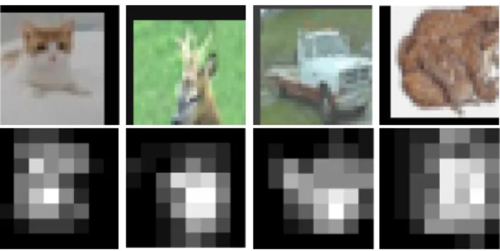
In precision gating, we expect that the model will learn to compute features whose prediction values exceeding the threshold in high-precision while keeping others computed at low precision. In the image recognition task, we expect that high-precision features are mostly in the region where an object lies. To provide evidence that the precision gating can effectively learn to identity those regions, in Figure 5, we visualize the decision maps extracted from the final convolutional layer that is modified to support precision gating in the ResNet-18 model. A decision map is a gray scale 2D image that has the same spatial size as the output feature map in the same convolutional layer. The brighter a pixel is in the decision map, the more probably the same spatial location in the output feature map will be computed in high precision. The first row contains the original input images in CIFAR-10, and their corresponding decision maps are shown in the second row. We can see clearly that in each decision map, the locations of bright pixels roughly align with the object in the original image, which is exactly what we expect.
Figure 5: Visualization of gating probability –Top: feature maps from the final precision gating block in ResNet-18 on CIFAR-10. Bottom: probability of computing in high-precision (brighter pixel means higher probability). PG effectively identifies the location of the object of interest and increases bitwidth when computing in this region.