Project Scheduling with Time Windows

Project Scheduling

with Time Windows

Contributions to Management Science

H. DyckhoffKJ. Finke

Cutting and Packing in Production and Distribution

1992. ISBN 3-7908-0630-7 R. Flavell (Ed.)

Modelling Reality and Personal Modelling

1993. ISBN 3-7908-0682-X M. HofmannlM. List (Eds.) Psychoanalysis and Management 1994. ISBN 3-7908-0795-8 R. L. D'EcclesialS. A. Zenios (Eds.) Operations Research Models in Quantitative Finance 1994. ISBN 3-7908-0803-2 M. S. CatalaniIG. F. Clerico Decision Making Structures 1996. ISBN 3-7908-0895-4 M. Bertocchi~E. CavalliIS. Koml6si (Eds.)

Modelling Techniques for Financial Markets and Bank Management 1996. ISBN 3-7908-0928-4 H. Herbst

Business Rule-Oriented Conceptual Modeling

1997. ISBN 3-7908-1004-5 C. Zopounidis (Ed.)

New Operational Approaches for Financial Modelling

1997. ISBN 3-7908-1043-6 K. Zwerina

Discrete Choice Experiments in Marketing

1997. ISBN 3-7908-1045-2 G. Marseguerra

Corporate Financial Decisions and Market Value

1998. ISBN 3-7908-1047-9

A. Scholl

Balancing and Sequencing of Assembly Lines

1999. ISBN 3-7908-1 180-7 E. Canestrelli (Ed.)

Current Topics in Quantitative Finance

1999. ISBN 3-7908-1231-5

W. BiihlertH. HaxiR. Schmidt (Eds.) Empirical Research on the German Capital Market

1999. ISBN 3-7908-1 193-9 M. BonillatT. CasasuslR. Sala (Eds.) Financial Modelling

2000. ISBN 3-7908-2282-X S. Sulzmaier

Consumer-Oriented Business Design 2001. ISBN 3-7908-1366-4

C. Zopounidis (Ed.) New Trends in Banking Management

2002. ISBN 3-7908-1488-1

WHU Koblenz - Otto Beisheim Graduate School of Management (Ed.)

Structure and Dynamics of the German Mittelstand

Ulrich Dorndorf

Project Scheduling

with Time Windows

From Theory to Applications

With

21

Figures and

17

Tables

Phy

sica-Verlag

Series Editors Werner A. Muller Martina Bihn Author

Dr. Ulrich Dorndorf

INFORM - Institut fur Operations Research und Management GmbH PascalstraSe 23 52076 Aachen Germany [email protected] ISSN 1431-1941

ISBN 3-7908-1516-0 Physica-Verlag Heidelberg New York Cataloging-in-Publication Data applied for

Die Deutsche Bibliothek - CIP-Einheitsaufnahme

Dorndorf, Ulrich: Project scheduling with time windows: from theory to applications; with 17 tables I Ulrich Dorndorf. - Heidelberg; New York: Physica-Verl., 2002

(Contributions to economics) ISBN 3-7908-1516-0

Zugl. Diss., TU Darmstadt, Kennziffer Dl7

This work is subject to copyright. All rights are reserved, whether the whole or part of the material is concerned, specifically the rights of translation, reprinting, reuse of illustrations, recitation, broadcasting, reproduction on microfilm or in any other way, and storage in data banks. Duplication of this publication or parts thereof is permitted only under the provisions of the German Copyright Law of September 9, 1965, in its current version, and permission for use must always be obtained from Physica-Verlag. Violations are liable for prosecution under the German Copyright Law.

Physica-Verlag Heidelberg New York

a member of Bertelsmannspringer Science+Business Media GmbH

0 Physica-Verlag Heidelberg 2002 Printed in Germany

The use of general descriptive names, registered names, trademarks, etc. in this publication does not imply, even in the absence of a specific statement, that such names are exempt from the relevant protective laws and regulations and therefore free for general use.

Softcover Design: Erich Kirchner, Heidelberg

Acknowledgements

In the preparation of this work I am greatly indebted to the following people who have given freely of their time and shared their insights to assist in this effort. I am grateful to my advisors Prof. Dr. Wolfgang Domschke and Prof. Dr. Erwin Pesch, whose exceptional encouragement and support, kindness and patience have made this research a most valuable experience. I am indebted to T o h Phan Huy for many helpful, inspiring and enjoyable discussions, which helped improve this work con- siderably, and for carefully reading drafts of several chapters. I am also indebted to Werner Siemes for his help in the evaluation of the gate scheduling algorithm. I also want to thank Thomas Schmidt for his kind support. Most importantly, my special thanks goes to my family, without whose support this book could never have been completed.

Contents

1 Introduction 1

1.1 Motivation and Objectives

. . .

1

1.2 Outline

. . .

4

2 Optimisation Model 7 2.1 The General Single-Mode Model

. . .

8

2.1.1 Activities and Resources

. . .

8

2.1.2 Temporal Constraints

. . .

9

2.1.3 The Model

. . .

13

2.1.4 Schedules and Performance Measures

. . .

14

2.1.5 Domains of Decision Variables

. . .

15

2.1.6 Special Cases

. . .

15

2.2 Extension to Multiple Execution Modes

. . .

16

2.2.1 Modes

. . .

16

2.2.2 Resources

. . .

17

2.2.3 The Model

. . .

18

3 Constraint Propagation 19 3.1 Constraint Satisfaction and Optimisation

. . .

19

3.1.1 The Constraint Satisfaction Problem

. . .

20

3.1.2 The Constraint Optimisation Problem

. . .

21

3.1.3 Constraint Graphs

. . .

21 3.2 Concepts of Consistency

. . .

22 3.2.1 k-Consistency

. . .

22 3.2.2 Domain-Consistency

. . .

24 3.2.3 Bound Consistency

. . .

24 3.3 Consistency Checking

. . .

25 3.3.1 Consistency Tests

. . .

25

3.3.2 Consistency Checking Algorithms

. . .

26

3.3.3 Uniqueness of the Fixed Point

. . .

28

...

V l l l CONTENTS

4 Consistency Tests 31

4.1 Basic Concepts

. . .

32

4.2 Consistency Tests for Temporal Constraints

. . .

34

4.3 Interval Consistency

. . .

36

4.4 Disjunctive Sub-Problems

. . .

38

4.4.1 Disjunctive Activity Pairs

. . .

38

4.4.2 Selection of Disjunctive Sub-Problems

. . .

40

4.5 Disjunctive Interval Consistency Tests

. . .

41

4.5.1 InputlOutput Test

. . .

41

4.5.2 Input-or-Output Test

. . .

45

4.5.3 InputIOutput Negation Test

. . .

48

4.5.4 Summary and Generalisation

. . .

49

4.5.5 Relation to Interval Consistency

. . .

50

4.5.6 Lower Level Consistency

. . .

52

4.5.7 Sequence Consistency Does Not Imply k-b-Consistency .

.

54

4.5.8 Shaving

. . .

55

4.6 Cumulative Interval Consistency Tests

. . .

56

4.6.1 Unit-Interval Consistency

. . .

56

4.6.2 Activity Interval Consistency

. . .

57

4.6.3 Minimum Slack Intervals

. . .

60

4.6.4 Fully and Partially Elastic Relaxations

. . .

61

4.7 Multi-Mode Consistency Tests

. . .

62

4.8 Summary

. . .

64

5 A Branch-and-Bound Algorithm 67 5.1 Previous Solution Approaches

. . .

68

5.2 Constraint Propagation

. . .

70

5.2.1 Consistency Tests

. . .

70

5.2.2 Some Properties of the Earliest Start Times

. . .

70

5.3 The Branch-and-Bound Algorithm

. . .

71

5.3.1 The Branching Scheme

. . .

71

5.3.2 Upper and Lower Bounds

. . .

77

5.3.3 Some Properties of Active Schedules

. . .

78

5.4 Computational Experiments

. . .

80

5.4.1 Implementation of the Algorithm

. . .

80

5.4.2 Bidirectional Planning

. . .

80

5.4.3 Characteristics of the Test Sets

. . .

81

5.4.4 Experiments for the Problem PSltemplC,,

. . .

83

5.4.5 Experiments for the Problem PSlprecl C,,

. . .

93

. . .

5.5 Summary 100

6 Multi-Mode Extension of the Branch-and-Bound Algorithm 103

. . .

6.1 Previous Work 103

. . .

6.2 Constraint Propagation 105

. . .

CONTENTS ix

7 Applications in Airport Operations Management 109

. . .

7.1 Scheduling of Ground Handling Operations 110

. . .

7.2 Gate Scheduling 112

. . .

7.2.1 Introduction 112

. . .

7.2.2 Literature Review 115

. . .

7.2.3 Problem Description 116

. . .

7.2.4 Constraint Propagation 124

. . .

7.2.5 A Branch-and-Bound Algorithm 124

. . .

7.2.6 Lower Bounds 127

. . .

7.2.7 Problem Partitioning 129

. . .

7.2.8 Layered Branch-and-Bound 133

. . .

7.2.9 Large Neighbourhood Search 135

. . .

7.2.10 Computational Experiments 136

8 Summary and Conclusions 143

List of Figures 147

List of Tables 149

List of Symbols 151

Chapter

1

Introduction

1 . Motivation and Objectives

Project scheduling is concerned with the allocation of resources over time to perform a collection of activities. The decision models that fit within this framework cover a multitude of practical problems that arise, for example, in such diverse areas as research and development, software engineering, construction engineering, repair and maintenance, as well as make-to-order and small batch production planning. A project is a one-of-a-kind undertaking with specific objectives that has to be per- formed within a certain time-frame and with limited resource supply. Its manage- ment roughly consists of (1) a project definition and data acquisition phase, (2) a scheduling phase and (3) an execution and termination phase during which the sched- ule is realised and the performance is analysed.

This work deals with the scheduling aspect. The aim is to develop methods for finding an optimal schedule for a project; this involves the assignment of activities to resources and the definition of exact activity start and completion times, a task that is generally difficult whenever multiple activities simultaneously compete for the same resources. We will not address the topics related to the conception, selection, and definition of a project, but will rather assume that the project structure is given, including data on resource availabilities and requirements as well as the necessary processing times. Likewise, we will not deal with the issues that typically arise during the realisation phase of a project.

We shall investigate a very general class of deterministic project scheduling problems that is expressive enough to capture many features commonly found in practical problems, such as precedence constraints, activity time windows, fixed activity start times, synchronisation of start or finish times, maximal or minimal activity overlaps, non-delay execution of activities, setup times, or time varying resource supply and demand.

2 CHAPTER 1. INTRODUCTlON In the basic model, technological or organisational requirements are represented through generalised precedence constraints that allow to specify minimal andlor maximal time lags, or time windows, between any pair of activities. An activity may require different amounts of several resource types. Resource requirements and availabilities may vary in discrete steps over time. While we usually consider the objective of minimising the overall completion time of a project, most of the results apply at least for any performance measure that is a non-decreasing function of the completion or start times of the activities. We will also address multi-mode schedul- ing, i.e., the situation where a choice must be made between several modes in which an activity may be processed, reflecting time-resource or resource-resource tradeoffs. Due to its generality, the basic model also covers many difficult special problems that have been extensively studied in scheduling research, for example, shop scheduling problems (Blazewicz et al. 1996).

Throughout this work, we study deterministic project scheduling problems, where all parameters that define a problem instance are known with certainty in advance. Deterministic scheduling models are best suited if any possible random influences in the project execution phase can be expected to be low, and if the problem parameters can thus be estimated with high accuracy. This may, for instance, be the case if the activities of a project show a high degree of similarity with previous projects. In situations where the problem parameters are difficult to estimate and are subject to significant random influences, the use of deterministic scheduling techniques may, however, be problematic. As a typical example, deterministic scheduling in the pres- ence of stochastic activity processing times generally leads to an underestimation of the expected project duration, as already observed by Fulkerson (1962).

The first models and methods for dealing with large scale projects have been devised in the late 1950's and early 1960's. The well known Critical Path Method (CPM, Kelley 1961) and the Metra Potential Method (MPM, Roy 1962) have been designed for deterministic project scheduling with ordinary or generalised precedence con- straints, respectively, while the Project Evaluation and Review Technique (PERT, Malcolm et al. 1959) considers probabilistic activity processing times; the Graph- ical Evaluation and Review Technique (GERT, Pritsker and Happ 1966) addition- ally takes probabilistic precedence relations into account. These approaches have received great attention in the following years. In the early 1970's, Davis (1973) already reported more than 15 books and 300 papers on the subject.

The original models and methods simplified the problem by concentrating only on temporal constraints, i.e., by assuming that the availability of resources is not a lim- iting factor. Beginning in the late 1960's, the models were extended by additionally considering scarcity of resources. In order to distinguish between the classic CPM, MPM, and PERT or GERT models on the one hand and models that consider limited resource availability on the other hand, the latter are usually referred to as resource- constrained. The underlying problems are much more difficult to solve, as the com- putational effort for finding an optimal solution usually grows exponentially with the problem size. For a long time, this has prohibited the use of exact algorithms for scheduling large practical projects with resource constraints.

I. I. MOTNATOAJ AND OBJECTIVES 3

In the past years, interest and research efforts in the field of resource-constrained project scheduling have strongly increased, and many new modelling concepts and algorithms have been developed. Overviews of the advances in models and solu- tion methods are given in the survey papers of Brucker et al. (1999), Herroelen et al. (1998), Kolisch and Padman (2001), Drexl et al. (1997), Elmaghraby (1995), 0zdamar and Ulusoy (1995), Icmeli et al. (1993), or Domschke and Drexl (1991). A gentle introduction to network models for project planning and control is given by Elmaghraby (1977). Descriptions of the basic classic project scheduling models for the temporal analysis of projects can be found in many introductory Manage- ment Science textbooks (e.g. Domschke and Drexl 1998). Applications within the area of production planning have been described, e.g., by Hax and Candea (1984) and Giinther and Tempelmeier (2000); Drexl et al. (1994) discuss a special type of project scheduling software, called Leitstand system, for make-to-order manufactur- ing management.

The resource-constrained project scheduling problems studied in this work can be understood as extensions of the basic problem covered by the Metra Potential Method. Due to the general form of the temporal constraints, the resource-con- strained version of the problem is particularly difficult to solve. Even the question for the existence of a feasible schedule can in general only be answered with expo- nentially growing effort. This may be one the main reasons why, despite the expres- siveness and high practical relevance of the models, very few attempts have so far been made to design solution procedures for this class of problems.

The main objective of this work is to help overcome this deficiency by developing effective and efficient solution methods. The focus will be on the design and eval- uation of exact branch-and-bound algorithms for finding optimal schedules, but we shall also study the performance of heuristics based upon truncated versions of these procedures.

The scheduling methods that will be developed make use of a general purpose prob- lem solving paradigm that originated in the area of Artificial Intelligence. Constraint propagation is an elementary technique for simplifying difficult search and optimi- sation problems by exploiting implicit constraints that are discovered through the repeated analysis of the domains of decision variables and the interrelation between the variables and domains that is induced by the constraints. In the past years, con- straint propagation techniques have been applied with growing success for solving a number of difficult, idealised scheduling problems, mostly in the area of machine scheduling. The successful application for solving special cases of the general prob- lem class studied here suggests that the approach may also be valuable in this con- text. As a second objective of this work, we shall therefore study the application of constraint propagation techniques in project scheduling.

A third objective is to demonstrate the practical relevance of the approach taken in this work. To this end we shall describe possible applications of the models and methods and extensions thereof in the area of airport operations management.

CHAPTER 1. INTRODUCTION

1.2 Outline

The presentation of the results is organised as follows.

Chapter 2 introduces a decision model for deterministic project scheduling with gen- eralised precedence constraints, the basic problem considered in this work. The chapter starts with a description of the entities that make up a project scheduling problem: activities, resources, precedence relations or time windows, and perfor- mance measures. After presenting a formal optimisation model, the concept of do- mains, i.e., sets of possible values of decision variables, is introduced. The general problem is then related to some well known special cases that are obtained if certain assumptions about the resource availability and requirements andlor the structure of the precedence relations are made. Finally, the generalisation to multiple activity execution modes is described.

Chapter 3 gives a general introduction to constraint propagation. Constraint propa- gation is a search space reduction technique that tries to remove inconsistent values from the variable domains, i.e., values that cannot participate in any feasible solu- tion, by repeated applying a set of consistency tests. The chapter discusses different

concepts of consistency that have been developed in the literature on the constraint

satisfaction problem, and which may serve as a theoretical background for the prop- agation techniques that will be employed. Consistency checking methods are de- scribed that control the repeated application of the tests until a fixed point is reached, i.e., until no further reductions are possible. The chapter concludes by pointing to constraint programming environments that build upon the concepts that have been introduced.

Chapter 4 is devoted to consistency tests for project scheduling that may be applied within the general framework introduced in the preceding chapter. It first describes simple tests that analyse the precedence constraints of a problem. The emphasis of the chapter is on interval consistency tests that are based upon the comparison of the resource supply and demand within certain time intervals. Previous research has shown that difficult project scheduling problem instances are frequently char- acterised by a low resource availability, which leads to the existence of many dis-

junctive sub-problems, i.e., sub-problems with unit resource availabilities and re-

quirements. The chapter shows how disjunctive sub-problems can be identified and selected. Consistency tests that have been proposed in the literature for disjunctive (machine) scheduling problems are then reviewed and presented within a unifying framework using numerous examples. Previous results are generalised and related to the concept of interval work, i.e., the minimum amount of work that must be performed within a time interval. The search space reduction that is achieved by ap- plying the tests within a fixed point propagation method is analysed and related to the theoretical concepts of consistency presented in Chapter 3. The results for disjunc- tive sub-problems are then extended for the case of arbitrary resource availabilities and requirements. The chapter finally shows how the results can be used for multi- mode project scheduling by considering a mode-minimal problem instance, where

all mode-dependent problem parameters are replaced with the minimum possible values.

Chapter 5 describes a new time-oriented branch-and-bound procedure for the basic single-mode project scheduling problem, in which the constraint propagation tech- niques are embedded. The solution method enumerates possible activity start times by scheduling activities as early as possible or delaying them by reducing their start time domains in such a way that the construction of non-active (dominated) sched- ules is avoided. The procedure heavily relies upon the application of constraint prop- agation techniques at the nodes of the search tree. The algorithm is evaluated for the problem with generalised precedence constraints as well as for the special case of or- dinary (finish-start) precedence constraints, using many large sets of benchmark test problems from the literature with up to five hundred activities,per problem instance. The results are compared to those of other exact procedures that have recently been proposed as well as to heuristic results; a detailed analysis of the influence of certain parameters that characterise a problem instance is given.

Chapter 6 extends the branching scheme for the case of multi-mode project schedul- ing. The basic idea is to integrate a time-oriented branching over activity start times with a branching over mode assignments or restrictions.

Chapter 7 discusses applications of the models and methods in the area of airport operations management. We first describe an application of single-mode project scheduling with time windows in ground handling, where activities required for ser- vicing an aircraft while on the ground have to be scheduled. The focus of the chapter then is on the development of a model and solution procedure for gate scheduling, i.e., the problem of assigning flights (activities) to airport terminal gates or parking positions (modes) and scheduling the start and end times of the assignments. The chapter demonstrates how this problem can be modelled as a special multi-mode project scheduling problem with time windows. A solution procedure based on the

concepts and techniques developed in the preceding chapters is described and evalu- ated on large practical test-cases.

Chapter 2

Optimisation Model

This chapter describes an optimisation model for deterministic resource-constrained project scheduling with generalised precedence constraints. It introduces the ba- sic elements of project scheduling models such as activities, resources, precedence constraints, as well as performance measures for evaluating the cost or utility of a schedule.

We are concerned with scheduling a set of activities subject to constraints on the availability of several shared resources and temporal constraints that allow to spec- ify minimal and maximal time lags between the start of two activities. The objective considered in this work usually is to minimise the makespan, i.e., the maximum of the completion times of all activities, although most of the results hold for any regular objective function and are frequently also useful for optimising non-regular objective functions1_{. The rationale behind the makespan criterion is that an early completion} of the project is advantageous in the sense that it frees resources for other tasks and reduces the risk of deadline violations and associated penalties; furthermore, signif- icant payments are often linked to the project completion, and an early completion thus tends to increase the net present value of a project.

Sometimes, a choice can be made between several modes in which an activity can be processed. The modes may differ with respect to resource requirements and process- ing time, and they can influence the tightness of the temporal constraints; the modes reflect time-resource and resource-resource tradeoffs. Models with multiple possible execution modes per activity are called multi-mode models; otherwise we speak of single-mode models.

Using the classification scheme for project scheduling proposed by Brucker et al. (1999), which extends the well known three-field classification scheme for machine scheduling introduced by Graham et al. (1979), we will denote the main single-mode problem considered in this work with PSltemplC,,,,,, for ( a ) project scheduling with

'Chapter 7 develops a special project scheduling model for a specific application with a non-regular objective function.

8 CHAPTER 2. OPTIMISATION MODEL

(p)

general temporal constraints and (y) the objective of minimising the maximum completion time. In the alternative classification scheme developed by Herroelen et al. (1999) the problem can be characterised as m, llgprlCm,,. The multi-mode extension of the problem will be denoted with MPSJtempl C,,.

The problem PSltempl C,,, is sometimes referred to as resource-constrained project scheduling problem (RCPSP) with time windows (e.g. Bartusch et al. 1988), RCPSP with generalised precedence relations (e.g. De Reyck and Herroelen 1998), or RCPSP with minimal and maximal time lags (RCPSPImax, e.g. Schwindt 1998b). While the classic resource-constrained project scheduling problem with simple precedence constraints, i.e. the problem PSlpreclC,,, has been extensively studied, algorithms for solving the problem PSltempl C,,, or its multi-mode generalisation have only recently received growing attention in the literature, as documented by the recent surveys by Brucker et al. (1999), Herroelen et al. (1998), and Kolisch and Pad- man (2001). This may to some extent have been caused by the fact that the problem

PSlpreclC,,, itself is intractable and belongs to the class of NP-hard optimisation

problems (Blazewicz et al. 1983). As an extension, the problem PSltemplC,, is, of course, also NP-hard, and even the question whether a problem instance has a feasi- ble solution is NP-complete in the strong sense (Bartusch et al. 1988)~. As a gener- alisation of the problem PSItempIC,,, the multi-mode problem MPSlternplC,,, and its corresponding feasibility problem belong to the same complexity class.

In the following, we will first describe the single-mode project scheduling problem

PSltemplC,, in detail in Section 2.1 and then introduce its multi-mode version in

Section 2.2.

2.1

The General Single-Mode Model

2.1.1 Activities and Resources

The basic entities of the project scheduling problem considered are the activities or jobs. A set of activities V = (1,.

.

.

,

n ) has to be processed with the objec- tive of minimising the makespan, which is the maximum of the completion times of all activities. Each activity i E V has a specific processing time pi and a start time

Si.

While the former is fixed in advance, the latter is a decision variable. The completion time of an activity is denoted with C i . Because the processing times are fixed and deterministic, the completion time of an activity follows from its start time. By choosing sufficiently small time units we can always assume that the pro- cessing and start and completion times are non-negative integer values. We study

the non-preemptive version of the problem, which means that activities must not be

interrupted during their processing.

2 ~ ~ - c o m p l e t e n e s s of the feasibility problem is shown by transformation of an NP-complete unit- time scheduling problem Q. NP-completeness in the strong sense follows from the fact that Q is not a number-problem.

2.1. THE GENERAL SINGLE-MODE MODEL 9

An activity i requires rik E No units of one or several resources

k

E R, where R

denotes the set of all resources. For the sake of simplicity we assume that resource

k

is available in constant amount R n , although the results derived in the subsequent sections also apply if we consider variable resource supply instead: for constant

R k , time varying resource supply can easily be modelled by introducing fictitious activities (Bartusch et al. 1988). Resources may not be shared and are exclusively assigned to an activity during its processing. They are reusable, i.e., they are released when they are no longer required by an activity and are then available for processing other activities. More precisely, an activity uses exactly rik units of resource k in any interval of width one starting at time t = S i ,

. . . ,

Si

+

pi - 1, at which these units are not available for other activities, and releases them at time t = Si +pi. The set of activities which require resource k is denoted with Vk := {i E V

I

rir,

>

0 ) . A resource k E R with supply Rk

>

1 is also called cumulative resource; in the special case where R k = 1 we speak of disjunctive or unary resources, which are sometimes also referred to as machines.

Resource constraints ensure that in any processing period the resource demand never exceeds the resource supply. It is possible to define these resource constraints in a quite elegant way using the concept of a slackfunction, which will be introduced in Chapter 4. For the time being it is sufficient to define the auxiliary set V ( t ) of activities in process at time t , or more precisely, in the right-open interval [t, t

+

l[. The resource constraints can then be stated as follows:

A schedule, i.e., an assignment of activity start times Si,

.

. .

,

S,, is resource feasible if it satisfies the above constraint.

1

2.1.2

Temporal Constraints

In general, activities cannot be processed independently from each other due to scarcity of resources and additional technological requirements. Technological re- quirements will be modelled by temporal constraints or, as synonyms, generalised precedence constraints or time windows. Many classic scheduling models such as the well known resource-constrained project scheduling problem, which is a special case of the model described here, only use minimal time lags between activities; the lags reflect finish-start precedence relations between activities and are thus assumed to be equal to activity processing times. Arbitrary minimal and maximal time lags are an important generalisation, as they allow to model many characteristics commonly found in practical scheduling problems. The temporal constraints can for instance be used to model activity time windows, fixed activity start times, synchronisation of start or completion times, maximal or minimal activity overlaps, non-delay execu- tion of activities, setup times, or time varying resource supply and demand (Bartusch et al. 1988, Elmaghraby and Kamburowski 1992, Neumann and Schwindt 1997).

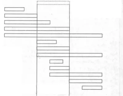
CHAPTER 2. OPTIMISATION MODEL 1 i before j 2 i meets j 3 i overlaps j 4 i finishedby j 5 i contains j 6 i starts j 7 i equals j 8 i started by j 9 i during j 10 i finishes j 1 1 i overlapped by j 12 i met by j 13 i after j I position of activity i ... I ... i position of activity j

Figure 2.1 : Possible temporal relations between two activities

Figure 2.1 shows the thirteen possible temporal relations between a pair of activities (Allen 1983)'. We will see that generalised precedence constraints can selectively enforce or admit any of these relations; this stands in contrast to precedence con- straints with minimal time lags only and simple completion-start precedence con- straints.

A generalised precedence constraint (i, j ) specifies a minimal or maximal time lag between two activities i and j and has the general standardised form:

As for the activity start and processing times, we will. assume without loss of gen- erality that all time lags dij are integer values. If dij

>

0 then the constraint (i, j ) can be interpreted as: activity j must start at least dij time units after the start of

i (minimal time lag). If d i j

5

0, then the following interpretation applies: j must start at most d i j time units before the start of i (maximal time lag). The set of all generalised precedence constraints is denoted with E .

2.1. THE GENERAL SINGLE-MODE MODEL

dji

<

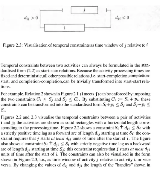
0

Figure 2.2: Visualisation of temporal constraints as forward and backward arcs

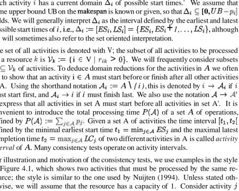
Figure 2.3: Visualisation of temporal constraints as time window of j relative to i

Temporal constraints between two activities can always be formulated in the stan- dardised form (2.2) as start-start relations. Because the activity processing times are fixed and deterministic, all other possible relations, i.e. start-completion, completion- start, and completion-completion, can be trivially transformed into start-start rela- tions.

For example, Relation 2 shown in Figure 2.1 (i meets j) can be enforced by imposing the two constraints Ci

5

S j and S j

5

Ci. By substituting Ci := Si + p i , these constraints can be transformed into the standardised form Si +pi

5

S j and S j -pi

5

si

.

Figures 2.2 and 2.3 visualise the temporal constraints between a pair of activities i and j; the activities are shown as solid rectangles with a horizontal length corre- sponding to the processing time. Figure 2.2 shows a constraint Si

+

dij

5

S j with a strictly positive time lag as a forward arc of length dij starting at time Si; the con- straint requires that j starts at least dij units of time after the start of i. The figure also shows a constraint S j

+

d j i

5

Si with strictly negative time lag as a backward arc of length dji starting at time S j ; this constraint requires that j starts at most dji

units of time after the start of i. The constraints can also be visualised in the form shown in Figure 2.3, i.e., as time window of activity j relative to activity i, or vice versa. By changing the values of d i j and d j i the length of the "handles" shown in

12 CHAPTER 2. OPTLMISATTON MODEL

Figure 2.3 can be adjusted and the size or position of the relative time window is changed. For simplicity, Figures 2.2 and 2.3 use only two activities for visualis- ing minimal and maximal time lags. In general, the time lags may lead to cycles involving an arbitrary number of activities.

Many special cases of the problem PSltemplC,,,, do not allow for negative time lags and cyclic temporal constraints. In the terms of Figure 2.3 this corresponds to removing the right handle labelled d j i .

Using the time window visualisation, it is easy to see that any of the thirteen possi- ble relations shown in Figure 2.1 can either be selectively enforced or be admitted or ruled out by choosing suitable minimal and maximal time lags (and, of course, processing times).

The set of all temporal constraints can be visualised in an activity-on-node network or digraph G(V, E) with vertex set V and edge set E with edge weights d i j , where minimal lags are usually represented as forward edges and maximal lags as backward edges4_{. The vertices of G correspond to the activities of the project, and there are} edges between any two activities (vertices) i and j that are linked by a precedence constraint (i, j) E E . Frequently, two fictitious activities 0 and n

+

1 that represent the start and end of a project are added as source and sink of the network, with edges from the source to all real activities and from all real activities to the sink, with edge weights do,i = 0 and di,n+l = pi, for i = 1,

. . .

,

n. For the remainder of this section we will assume that G contains the fictitious start and end activities.

A time feasible schedule, i.e., one that satisfies all temporal constraints, is an assign- ment of non-negativenumbers to the activity start times S1

,

.

.

.

,

s,, or, equivalently,

to the vertices of G, such that

The numbers fulfilling (2.3) are also called potentials in graph theory (Berge 1985), and there is a well developed theory about them that also forms the basis of the Metra-Potential-Method (MPM) for project networks (Roy 1962), which deals with start-start time lags and also covers the temporal constraints of the model discussed here.

It is well known that there exists a time feasible schedule (a potential for G) iff

G has no directed circle of positive length (Bartusch et al. 1988). Such a cycle would correspond to a logical contradiction in the temporal constraints. For example, consider a cycle involving only two activities that is formed by the constraints Si

+

3

5

Sj and S j - 2

<

S i ; the length of the cycle is 1; while the first constraint requires that activity j starts at least 3 units of time after i, the second constraint demands that i starts at most 2 units before j.

The existence of a time feasible schedule can be tested by computing the unique component-wise minimum solution of (2.3), which gives the earliest possible starting

4 ~ o r all graph theoretic notions not defined here see LawIer (1976). For an introduction to network representations of projects see Elmaghnby (1977).

2.1. THE GENERAL SINGLE-MODE MODEL 13

times. This schedule, which is usually not resource feasible, is also called the earliest start schedule. The earliest start schedule can be efficiently computed by standard graph algorithms, e.g. with effort O(n3_{) by the Floyd-Warshall Algorithm (Lawler}

1976). Alternatively, the earliest start schedule can be derived through constraint propagation, as shall be explained in the following chapters.

2.1.3 The Model

The problem PSltemplC,, can now conceptually be stated as follows:

S i + d i j < S j , V ( i , . i ) E E , (ii)

CiEv(t)

rik

5

R k

,

V t E

No,

V k E

R,

(iii)

Vi E V . (i.1

A schedule S = (S1,

.

.

.

,

S,) is an assignment of all activity start times. S is feasible if it satisfies all precedence constraints (ii) and resource constraints (iii). Reformu- lating the problem, the task is to find a feasible schedule with minimal makespan. There are several other ways of formally modelling the problem PSltempJC,, that mainly differ in the way how resource constraints are represented. Many formula- tions have originally been proposed for the problem PSlpreclC,,,, i.e., the exten- sively studied variant of the problem PS(temp(C,,, where all time lags dij are equal to the activity processing times pi.

The formulations are frequently based on using time indexed binary decision vari- ables zit that take the value one if an activity i E V finishes in (or is processed in, or starts before, etc.) period t and zero otherwise. The first formulation of this type for the problem PSlpreclC,, has been described by Pritsker et al. (1969).

Other formulations are based on the concept of using forbidden sets (Bartusch et al. 1988) to represent the resource constraints. A forbidden set of activities is a set

N

S

V for which

rik

>

R I , for some k t R. i € N

Condition (2.4) is the negation of (2.1); it is time independent due to the constant resource demands and supplies. Given a set

N

of all forbidden sets, a schedule S is resource feasible iff no set N E

N

is scheduled simultaneously in any period t.

A disadvantage of the description by forbidden sets is the fact that the number of required (minimal) forbidden sets may grow exponentially with the problem size, although it seems that for many applications this does not cause problems (Stork and Uetz 2000).

14 CHAPTER 2. OPTIMISATION MODEL

Forbidden set formulations have been used, e.g., by Bartusch et al. (1988) and by Alvarez-Valdes and Tamarit (1993). A formulation based on the complementary concept of compatible sets of activities has been proposed by Mingozzi et al. (1998).

2.1.4

Schedules and Performance Measures

A schedule S = (Sl

,

.

.

. ,

Sn)

is an assignment of all activity start times. The quality of a schedule is usually measured by a cost or utility function n :

R

n

+

_IR

that transforms the vector of start or completion times onto a one-dimensional scale. The makespan function

C

,

,

:= n(S) := r n a x i ~ v Si

+

pi is an example of such a transformation.

When comparing two schedules S and S' we say that S

5

S' if no activity in S

starts later than in S':

Further, S

<

S' if S

5

S' and additionally at least one activity in

S

starts earlier:

A schedule S is active if it is feasible and if there exists no other feasible schedule S' such that S'

<

S . In other words, S is active, if no activity can be started earlier without violating either one of the precedence or resource constraints. If a schedule

S is not active and some activity i can therefore be started earlier than at time Si, then we say for short that i can be lefr-shifed in S.

A detailed discussion of active schedules and the related concepts of semi-active and

non-delay schedules in the context of project scheduling is given by Sprecher et al. (1995).

The definition of active schedules immediately leads to the following simple and well known observation: any solution method which minimises the makespan func- tion can refrain from generating non-active schedules, since there always exists a corresponding active schedule with a lower or identical makespan. We shall exploit this observation in the branch-and-bound procedure developed in Chapter 5.

The observation can be generalised for the class of regular measures of pel3cormance

(Conway et al. 1967) which is defined as the class of all objective functions that are non-decreasing with respect to the component-wise ordering of

R

n

_,

_{i.e., for which}

Regular measures of performance cover the standard objective functions used in scheduling such as makespan, weighted flowtime, or tardiness costs. The condition is general enough to allow for many cost terms that occur in practical applications. I

2.1. THE GENERAL SINGLE-MODE MODEL 15

2.1.5 Domains of Decision Variables

We will now introduce the concept of domains of decision variables, which will prove useful in the following chapters. Each activity start time variable Si has a current domain As,

c

No of possible values. Because the activity start times are the only decision variables in the single-mode model, we will also use the shorter notation Ai instead of As, when no confusion is possible and simply speak of the domain of activity i; we shall use the explicit notation when dealing with multi-mode models. We will later assume that some real or hypothetical upper bound UB on the optimal makespan is known or given, so that even Ai

C

[0,

UB

-

pi] holds. This is necessary, since most of the constraint propagation methods that will be applied can only deduce a domain reduction if the current domains are finite. If no initial upper bound is given we use the trivial upper bound

The set of current domains of all activities is denoted with A := {Ai

I

i E V). For an activity i E V, ESi(A) := min Ai is the earliest start time, ISi(A) := m a Ai the latest start time, &(A) := ESi (A)

+

pi the earliest completion time and LCi (A) := ISi(A) +pi the latest completion time of i. If no confusion is possible, then we will write ESi, I S i , etc., for short.

A schedule S is called domain feasible with respect to a set A of current domains if the current domain of each activity still contains the start time of this activity in S , i.e., if we can arrive at S by repeatedly reducing the current domains.

Given a set A of current domains, the set of all activities V can be naturally parti- tioned into a set of scheduled and non-scheduled, or free, activities. Clearly, if the current domain of an activity i contains exactly one entry, then i must start at that time and can be considered as scheduled. Hence

is the set of scheduled activities, and

is the set of free activities. For all scheduled activities i E VS(A), the start time is defined through Si (A) := ESi (A) = LSi (A).

2.1.6

Special Cases

The general problem PSItempI C,,, contains several special cases that are obtained if

the admissible precedence constraints are restricted in certain ways or if the resource supply takes a special form.

16 CHAPTER 2. OPZTWSATION MODEL

A first class of simple problems is obtained if the resource constraints are relaxed, i.e., if resource supply is unlimited. This first leads to a (resource-un-constrained) project scheduling problem with generalised precedence constraints, a problem that is addressed by the well known Metra-Potential Method (MPM) for the temporal analysis of project networks. The problem covered by the famous Critical Path Method (CPM) is obtained if, additionally, only simple precedence constraints are allowed, i.e., if the time lags dij between a pair of activities i and j are equal to the processing time of the preceding activity i: dij = Pi, V ( i , j) E E .

In contrast to the simple problems with unlimited resource supply, problems with resource constraints are generally difficult to solve.

One of the best studied special cases of the problem PSltempJC,, is the classic RCPSP with simple precedence constraints, i.e., the problem PSlpreclC,,,, which generalises the problem covered by the CPM method by adding resource constraints. It has been shown that several seemingly unrelated optimisation problems can be for- mulated as instances of the problem PSlpreclC,,. Examples include the bin pack- ing (Garey et al. 1976) and the assembly line balancing problem (Elmaghraby 1977, Sprecher 1994). The relation of the multi-mode problem MPSlprecl C,, to the knap- sack packing problem as well as to two- and three-dimensional packing and cutting problems has been discussed by Hartmann (1999).

The problem PSlpreclC,,,, with ordinary precedence constraints is in turn a gener- alisation of several well known, difficult optimisation problems studied in machine scheduling, where unary, or disjunctive, resources are considered. Examples include shop scheduling problems such as the job shop, flow shop, and open shop problems (Blaiewicz et al. 2001) as well as many other, more special problems. We will see in the following chapters that some solution techniques originally developed for shop scheduling can be successfully applied for solving project scheduling problems. A special problem that has been called Generalised RCPSP (Demeulemeester and Herroelen 1997a, Klein 2000b) is obtained if the RCPSP is extended by allowing for arbitrary minimal time lags, combined with the assumption that the precedence constraints are acyclic.5

2.2

Extension to Multiple Execution Modes

2.2.1 Modes

In multi-mode scheduling, an activity may be processed in one of multiple possible execution modes, which differ with respect to the necessary processing time and the resource requirements. Furthermore, the time lag between a pair of activities may

5 ~ h e fact that time lags of value zero are legal would otherwise allow for cycles of length zero, cor- responding to a synchronisation of start times; this would slightly complicate the design of enumeration schemes.

2.2. EXTENSION TO MULTIPLE EXECUTION MODES 17 vary depending on the chosen mode. The modes reflect tradeoffs between required processing time and resource consumption on the one hand as well as tradeoffs be- tween the consumption of different types of resources on the other hand; additionally the time lags between activities may vary depending on the chosen modes.

The mode Mi in which an activity

i

E V is processed thus becomes an additional decision variable, which can take values from the associated set M i of all admissible modes. The current domain of Mi is denoted with AM;, and initially

AM^

= M i .

As the processing time and resource requirements of an activity now depend on the chosen mode, they are indexed accordingly: pi, is the time required for processing activity i in mode p E M i , and ri,k is the amount of resource k E

R

needed for executing activity i in mode p. The mode dependent time lag that must pass between the start of two activities i, j E

V

if i is performed in mode p E M i and j in mode

v E

M j

is denoted with diPj,.

The initial mode domain of an activity can be reduced by removing inefficient modes. In multi-mode models with simple finish-start precedence constraints, a mode is called ineficient if its processing time is not shorter and its resource requirement is not less than that of another mode of the same activity. If generalised precedence constraints are allowed, this condition must be strengthened by additionally consid- ering the mode-dependent time lags: A mode p E AM; of activity i is inefficient if its processing time is not shorter and its resource requirement is not less than that of another mode of i and if the time lags diPjv and djvi, associated with mode p and activity i are not less than for another mode of i, for all j E V, for which (i, j) E &

or (j, i) E E, and all v E A M j .

2.2.2 Resources

In multi-mode project scheduling it is common practice to distinguish between re- newable and non-renewable resources, as originally proposed by Slowinski (1980) and Weglarz (1981).

So far, we have only introduced renewable resources, which are constrained on a per period basis. The required number of units of a renewable resource are assigned to

an activity during its processing; upon completion of the activity, the resource units are released again and are then available for processing other activities. Examples of renewable resources include manpower and machines.

Non-renewable resources are globally constrained for the entire planning horizon. In contrast to renewable resources, they are consumed by processing an activity and cannot be reused. Money is an example for a non-renewable resource. Non- renewable resources can thus be used to model budget constraints for a project. A non-renewable resource is redundant and may be removed if the mode-dependent maximal total demand for the resource is at most equal to the resource supply. Non- renewable resources need only be considered in multi-mode problems as they must

18 CHAPTER 2. OPTIMISATION MODEL

always be redundant in instances of single-mode problems (or the problem instance does not have a solution).

Resources that are constrained per period as well as for the entire project are called doubly constrained. A doubly constrained resource can be modelled by introducing a renewable and a non-renewable resource.

Another type of resource that allows to model resource supply restrictions for a sub- set of periods and that is called partially renewable has recently been proposed by Bottcher et al. (1999).

In the following we will distinguish between the set RP of renewable and the set

R" of non-renewable resources, i.e.,

R

= RP U RV

, and denote the supply of a renewable (non-renewable) resource k E R with R i (RL).

2.2.3 The Model

The problem MPSJtemplC,,,, can now conceptually be stated as follows:

min{max{Si

+

&Mi }} s.t.

zEV (i)

Si

+

d i ~ ; jMj

I

Sj, v(i, j ) E E, (ii)

CiEv(t)

T i ~ ~ k

5

RL, vt E No, vk E R P , (iii)

xiEv

7 ' i ~ ; k

5

Ri, vt No

,

\Jk

E R V , (iv)

si

E NO, Vi E V . (v)

Mi E

Mi,

Vi E

V.

( 4

A schedule (S, M ) = (S1,.

. . ,

S,, M I , .

. .

,

M,) is an assignment of all activity start times and modes. (S, M ) is feasible if it satisfies all precedence constraints (ii) and constraints for renewable (iii) and non-renewable (iv) resources.

The multi-mode project scheduling problem MPSltemplC,, can be conceptually divided into two sub-problems. The mode assignment problem consists of finding a mode vector that satisfies constraints (iv) and (vi); it is NP-complete for prob- lems with at least two non-renewable resources (Kolisch 1995). Given a mode- assignment, the scheduling sub-problem defined by (i) - (iii) and (v) is of the type PSI temp

1

Cmx.

Chapter

3

Constraint Propagation

The branch-and-bound algorithms that will be developed in the following chapters rely to a great extent on efficient constraint propagation techniques. Constraint prop- agation is a problem reduction technique that transforms problems into equivalent problems that are hopefully easier to solve. The basic idea is to reduce the search space of a problem instance through the repeated analysis and evaluation of variables, their domains, and the interdependence between the variables that is induced by the set of constraints. The goal is to detect and remove inconsistent assignments that can- not participate in any feasible solution. A whole theory is devoted to the definition of

different concepts of consistency, which may serve as a theoretical background for the propagation techniques that we will employ. This theory has been developed for

the constraint satisfaction problem (CSP) or constraint optimisation problem (COP);

the project scheduling problems examined in this work can be understood as special subclasses of the CSP or COP.

In this chapter we shall introduce the standard CSP and COP and the important con- cepts related to it. Section 3.1 gives a short introduction to these problem classes; Section 3.2 then describes different concepts of consistency, and Section 3.3 ad- dresses consistency checking algorithms. Section 3.4 points to some software sys-

tems and languages that have been developed based on concepts from CSP research and help in the formulation and solution of CSPs.

3.1

Constraint Satisfaction and Optimisation

A CSP is composed of a finite set of variables, each of which is associated with a finite domain, and a set of constraints that restrict the values that the variables can simultaneously take. The task is to assign a value from its domain to each variable so that all constraints are satisfied. The COP additionally requires that the solution optimises some objective function. The problem PSltemplC,,,, introduced in Chap-

20 CHAPTER 3. CONSTRAINT PROPAGATION

ter 2 is an example of a COP. Any COP can be transformed into a related CSP by replacing the objective function with a constraint on the objective value. By repeat- edly restricting the value, e.g. through bi-section over the interval defined by a bound on the objective function value and an initial guess for the optimal value, a COP can be solved by repeatedly solving related CSPs.

The CSP was first formalised and studied by Huffman (1971), Clowes (1971) and Waltz (1975) in vision research for solving line-labelling problems. Haralick and Shapiro (1979, 1980) and Mackworth (1992) discuss general algorithms and appli- cations of CSP solving. Hentenryck (1992) and Cohen (1990) tackle the CSP from a constraint logic programming viewpoint. Comprehensive introductions to the CSP are provided by Meseguer (1989), Kumar (1992) and Dorndorf et al. (2000b). An exhaustive overview of the theory of constraint satisfaction and optimisation is given by Tsang (1993). We will only present the necessary aspects and start with some basic definitions.

The finite domain of a variable is the set of all values that can be assigned to the vari- able. For many interesting problems, the assumption that the domains are finite is not a serious restriction. For example, for the project scheduling problems introduced in Chapter 2 the domains of the start and completion times can easily be made finite by imposing a bound on the makespan. The domain associated with the variable x is de- noted with A,. If V = 1x1,.

.

.

,

x,) is a set of variables and A = {A,,

, . . .

,

A,,,) the set of their domains, then an assignment a = ( al, .

. .

,

a,) is an element of the Cartesian product A,, x

. . .

x A,,, ; in other words, an assignment instantiates each variable xi with a value ai E A,; from its domain.

A constraint c on A is a function c : A,;, x

. . .

x A,;,

+

{true, false), where V' :=

{xil,

.

. .

,

xi,} is a non empty set of variables. The cardinality IV'I is also called the arity of c. If 1V'I = 1 or IV'I = 2 then we speak of unary and binary constraints,

respectively. An assignment a E A,, x

. . .

x A,,, satisfies c if c(ai,,

. . . ,

ai, ) = true. Given a set of current domains A, a constraint is called resolved if it is satisfied for all assignments a E A,, x

.

.

.

x AXn, otherwise it is (still) unresolved.

3.1.1

The Constraint Satisfaction Problem

An instance P of the constraint satisfaction problem (CSP) is defined by a tuple

P = (V, A, C), where V is a finite set of variables, A the set of associated domains and C a finite set of constraints on A. An assignment a is feasible if it satisfies all constraints in C. A feasible assignment is also called a solution of P. We denote with F ( P ) the set of all feasible assignments (solutions) of P.

Given an instance P of the CSP, the associated task is to find a solution a E 3 ( P ) or to prove that P has no solution.

The goal of constraint propagation is to transform a problem P into a reduced but equivalent problem P' that is easier to solve. The reduced problem P' usually differs from P in the sense that the variable domains are reduced or that new, redundant

3.1. CONSTRAINT SATISFACTION AND OPTIMISATION 21

constraints, which may help in deducing future domain reductions, have been added. Problem reduction is an iterative process; we will generally assume that A and C

refer to the current domain set and constraint set of the current reduced problem. Whenever we must explicitely refer to the original domain set and constraint set in

P to avoid confusion, we will use the notation AO _{and C O .}

3.1.2 The Constraint Optimisation Problem

As distinguished from the constraint satisfaction problem, the constraint optimisa- tion problem searches for a solution which optimises a given objective function. We will only consider the case of minimisation, as maximisation can be handled sym- metrically.

An instance of the constraint optimisation problem (COP) is defined by a tuple P =

( V , A , C , z ) , where (V, A , C ) is an instance of the CSP and z an objective function

z : A,, x

.

.

.

x A Z n

+

a.

Defining

Zmin(P) :=

otherwise,

an assignment a is called an optimal solution of P if a is feasible and z ( a ) = zmin(P).

Given an instance P of the COP, the associated task is to find an optimal solution of

P and to determine z,i, ( P ) .

The project scheduling problems introduced in Chapter 2 can be seen as special c o p s .

It is not hard to see that the CSP and the COP are intractable and belong to the class of NP-hard problems. For a more detailed discussion, which exceeds our needs, we refer to Garey and Johnson (1979) or Tsang (1993).

3.1.3 Constraint Graphs

An instance of the CSP can be represented by means of a constraint graph which vi- sualises the interdependencies between variables that are induced by the constraints. If we restrict our attention to unary and binary constraints then the definition of a con- straint graph

G

is quite straightforward. The vertex set of

G

corresponds to the set of all variables V , while the edge set is defined as follows: two vertices xi, xj E V,

i f j , are connected by an undirected edge if there exists a constraint c(xi, x j ) E C .

This can be generalised to constraints of arbitrary arity using the concept of hyper- graphs (Tsang 1993).

For a resource-un-constrained project scheduling problem that contains only prece- dence constraints the constraint graph of the problem has the same structure as the activity-on-node precedence network but is undirected.

22 CHAPTER 3. CONSTRAINT PROPAGAT7ON

3.2 Concepts of Consistency

As the domains of a CSP instance

P

are finite,

P

can in principle be solved by a simple generate-and-test algorithm that enumerates all assignments a E A,, x

. . .

x A,,, , verifies whether a satisfies all constraints c E C, and stops if the answer is "yes". The COP can be solved by enumerating all feasible assignments and storing the one with minimal objective function value.

Of course, this method is not practicable due to the size of the search space which grows exponentially with the number of variables. In the worst case, all assignments of a CSP instance have to be tested which cannot be carried out efficiently except for problem instances too small to be of any practical value. It is thus worth to look for methods that can reduce the search space prior to starting (or during) the search process.

One such method of search space reduction which only makes use of simple infer- ence mechanisms and which is not problem specific is known as constraintpropaga-

tion. The origins of constraint propagation go back to Waltz (1972) who almost three

decades ago developed a now well-known filtering algorithm for labelling three- dimensional line diagrams.

The basic idea of constraint propagation is to make implicit constraints more visi- ble through the repeated analysis and evaluation of the variables, domains and con- straints describing a specific problem instance. This makes it possible to detect and remove inconsistent variable assignments that cannot participate in any solution by

a merely partial problem analysis.

Over the years, different concepts of consistency have been developed that allow to identify inconsistent assignments. In this context, the term consistency with regard to certain properties must be understood in the following way: variable assignments, whose presence would cause these properties to be false, have been ruled out. The different types of consistency guarantee different properties. Roughly speaking, a concept of consistency defines the maximal search space reduction that is possible regarding some specific properties. It is worth pointing out that the term consistency as used here is neither a necessary nor a sufficient condition for a problem to be solvable.

The first concepts of consistency have been formalised by Montanari (1974) who introduced node-, arc- and path-consistency. Roughly speaking, these concepts are based on the examination of constraints containing k variables, where k = 1 , 2 , 3 ,

with their names being derived from the presentation of a CSP instance as a con- straint graph. These concepts have been generalised by Freuder (1978) to the notion

of k-consistency. We will describe the basic ideas of k-consistency in an informal