APPLICATION OF FUZZY LOGIC TO QUANTIFY THE UNCERTAINTY IN LAYER OF PROTECTION ANALYSIS
A Dissertation by YIZHI HONG
Submitted to the Office of Graduate and Professional Studies of Texas A&M University
in partial fulfillment of the requirements for the degree of DOCTOR OF PHILOSOPHY
Chair of Committee, M. Sam Mannan Committee Members, James Holste
Mahmoud El-Halwagi Reza Langari
Head of Department, M. Nazmul Karim
May 2017
Major Subject: Chemical Engineering
ii ABSTRACT
Layer of Protection Analysis (LOPA) is a widely used semi-quantitative risk assessment method. LOPA includes both frequency and consequence expressed in an order of magnitude approximation. Compared with Quantitative Risk Analysis (QRA), LOPA provides a simplified but less precise method to assess the effectiveness of protection layers and the risk reduction of an incident scenario. The outcome frequency and consequence of LOPA are intended to be conservative, which makes the risk overestimated. A high risk indicates the requirement of additional Independent Protection Layers (IPLs), which calls for higher installation and maintenance costs. There are different sources and types of uncertainty in LOPA model that need to be identified and quantified.
Fuzzy logic is a method to deal with systems that are too complex or not clearly defined. Using fuzzy arithmetic, imperfect data are analyzed in a natural and flexible way. Through the application of fuzzy logic, uncertainty from data and experience from experts can be quantified, and a more accurate and precise risk value can be obtained. Various types of fuzzy logic systems, including type-1 fuzzy logic and type-2 fuzzy logic are studied in this work.
The goal of this work is to increase the accuracy and precision of LOPA model while retaining its simplicity. A probabilistic and fuzzy logic hybrid approach is developed to deal with the uncertainty in failure rate data. This method facilitates a more accurate and precise failure rate database considering generic database, plant-specific data and
iii
expert experience. It has been applied to a distillation system, with a capacity to distill 40 tons of flammable n-hexane, and the results show that a more accurate failure rate can be achieved with the available data and expert judgment. Furthermore, a type-2 fuzzy logic risk matrix is developed to increase the precision of a risk matrix. This new method also provides an efficient way to aggregate several risk matrices into one universal risk matrix. Its application to aggregate three standard risk matrices has been shown through a case study.
This work demonstrates the effectiveness of applying fuzzy logic in quantifying uncertainty in layer failure data to be used in LOPA. Fuzzy logic can also be helpful in other types of risk assessment.
iv DEDICATION
To my father Caifu Hong, my mother Peili Jiang, and my wife Zhe Han, for their love and unconditional support, for being the main motivation to move forward and become a better person every day.
v
ACKNOWLEDGEMENTS
I would like to sincerely thank my committee chair, Dr. M. Sam Mannan, for his mentoring, which has gone beyond the academic level. His vision and inspiration for students to make a contribution in the process safety field motivated me throughout my research. I also thank him for giving me multiple opportunities to work on real world problems. His understanding during the difficult times is highly appreciated. I admire Dr. Mannan as a leader, a researcher, and a person.
I would like to offer my thanks to Dr. James Holste, Dr. Mahmoud El-Halwagi, and Dr. Reza Langari, for serving as my committee members, and for their guidance and support throughout the course of this doctoral research.
I would like to show my appreciation to Dr. Hans Pasman, Dr. Simon Waldram, and Dr. Maria Papadaki for giving me advice on my research project. I am sincerely thankful to them for their continuous advice and encouragement both in my research and life.
I would like to express my deep gratitude to Dr. Sonny Sachdeva and Dr. Noor Quddus for constant support and encourage throughout my graduate study. I am sincerely thankful to them for giving me insightful suggestions on my research.
I would also like to extend my thanks to the staff and members of the Mary Kay O’Connor Process Safety Center. Thanks to Valerie Green for her care and encouragement, to Alanna Scheinerman for her assistance in reviewing several manuscripts.
vi
There are not enough words to thank my parents, Caifu Hong, Peili Jiang, and my wife Zhe Han, for their love and unconditional support, for being the main motivation to move forward and become a better person every day.
vii TABLE OF CONTENTS Page ABSTRACT ...ii DEDICATION ... iv ACKNOWLEDGEMENTS ... v
TABLE OF CONTENTS ...vii
LIST OF FIGURES ... ix
LIST OF TABLES ...xii
1. INTRODUCTION ... 1
1.1. Uncertainty in LOPA ... 2
1.2. Chances vs. Fuzzy Logic ... 3
1.3. Dissertation Outline ... 4
2. BACKGROUND KNOWLEDGE OF LOPA ... 6
2.1. Risk Assessment ... 6
2.1.1. Hazard and Operability Study (HAZOP) ... 8
2.1.2. Failure Mode and Effects Analysis (FMEA) ... 9
2.1.3. Dow Fire and Explosion Index (F&EI) ... 9
2.1.4. Fault Tree Analysis (FTA) ... 10
2.2. Risk Matrix ... 10
2.3. Layer of Protection Analysis ... 12
3. BACKGROUND KNOWLEDGE OF FUZZY LOGIC ... 19
3.1. Classical Boolean Set ... 19
3.2. Type-1 Fuzzy Logic ... 23
3.2.1. Type-1 Fuzzy Set ... 24
3.2.2. Basic Operations and Properties ... 29
3.2.3. Type-1 Fuzzy Rules and Reasoning ... 31
3.2.4. Type-1 Fuzzy Modeling ... 38
3.3. Type-2 Fuzzy Logic ... 40
3.3.1. Type-2 Fuzzy Set ... 40
viii
Page
3.3.3. Basic Operations ... 46
3.3.4. Interval Type-2 Fuzzy Reasoning ... 47
3.3.5. Interval Type-2 Fuzzy Modeling ... 48
4. A PROBABILISTIC AND FUZZY LOGIC HYBRID APPROACH ... 51
4.1. Uncertainty Sources in Failure Rate ... 51
4.2. Relevant Literature Review and Gap Identification ... 53
4.3. Present Hybrid Approach ... 56
4.4. Case Study ... 69
4.5. Conclusions ... 76
5. UNIVERSAL RISK MATRIX ... 77
5.1. Uncertainty Sources in Risk Matrix ... 77
5.2. Literature Review and Gap Identification ... 79
5.3. Relevant Methods ... 80
5.3.1. Interval Approach (IA) ... 80
5.3.2. Linguistic Weighted Average (LWA) ... 85
5.4. Universal Risk Matrix Method ... 88
5.5. Case Study ... 92
5.6. Conclusions ... 98
6. CONCLUSIONS AND FUTURE WORK ... 99
6.1. Conclusions ... 99
6.1.1. Uncertainty in the Frequency ... 100
6.1.2. Uncertainty in the Risk ... 101
6.2. Future Work ... 102
ix
LIST OF FIGURES
Page
Figure 1. Diagrams for a Boolean set and a fuzzy set. ... 4
Figure 2. Spectrum of tools for risk-based decision making [28]. ... 8
Figure 3. Risk matrix example I. ... 11
Figure 4. Layers of protection for a possible incident [28]. ... 14
Figure 5. The process life cycle showing where LOPA is typically used [2]. ... 15
Figure 6. LOPA pictured as an event tree analysis [28]. ... 17
Figure 7. Diagrams for a Boolean set and a type-1 fuzzy set. ... 23
Figure 8. Membership function of a crisp set and a fuzzy set. ... 24
Figure 9. Core, support of a typical type-1 fuzzy set. ... 26
Figure 10. Membership function shapes [36]. ... 27
Figure 11. Membership function of three linguistic terms for Age. ... 28
Figure 12. Type-1 fuzzy set operations: intersection (AND), union (OR) and complement. ... 29
Figure 13. An example of type-1 fuzzy set and an α-cut. ... 33
Figure 14. Illustration of the T1 FS Decomposition Theorem when n α-cuts are used. ... 35
Figure 15. Mamdani fuzzy inference system. ... 37
Figure 16. Sugeno (TSK) fuzzy inference system. ... 38
Figure 17. The structure of type-1 fuzzy logic system. ... 38
Figure 18. Type-2 membership function as a blurred type-1 membership function [44]. ... 41
Figure 19. Type-2 fuzzy set example I. ... 42
x
Figure 21. Type-2 fuzzy logic example III. ... 44
Figure 22. (a) Type-1 fuzzy set; (b) Interval type-2 fuzzy set. ... 45
Figure 23. Standard interval type-2 fuzzy sets operations (a). Interval type-2 fuzzy set 𝐴 and 𝐵. (b). Standard union of 𝐴 and 𝐵. (c). Standard intersection of 𝐴 and 𝐵. ... 46
Figure 24. The structure of type-2 fuzzy logic system. ... 49
Figure 25. Structure of fuzzy logic and probabilistic hybrid approach. ... 56
Figure 26. Fuzzy modeling of parameter variance modifier (PVM). ... 58
Figure 27. Parameter Variance Modifier (PVM) membership function. ... 60
Figure 28. Database quality membership function. ... 61
Figure 29. Database relevance membership function. ... 61
Figure 30. Database applicability membership function. ... 61
Figure 31. Quantity of plant-specific data membership function. ... 62
Figure 32. Data confidence membership function. ... 62
Figure 33. Experience level of expert (year of working experience). ... 62
Figure 34. Fuzzy IF-Then rules of data relevance and database quality. ... 64
Figure 35. Fuzzy IF-Then rules of Data confidence. ... 65
Figure 36. Fuzzy IF-Then rules of PVM. ... 66
Figure 37. The resultant fuzzy surface of data applicability. ... 68
Figure 38. The resultant fuzzy surface of data confidence... 68
Figure 39. The resultant fuzzy surface of PVM. ... 69
Figure 40. A simplified distillation column system [36]. ... 71
Figure 41. Final failure rates in histograms for three scenarios with parameter variance modifier (PVM) equals 1, 0.8, 0.65 respectively. ... 75
xi
Figure 43. The flow diagram of Interval Approach. ... 81
Figure 44. The scale of frequency and an example of data interval. ... 82
Figure 45. The resultant interval type-2 fuzzy set of Risk Matrix I – Frequency B. ... 85
Figure 46. The flow to develop a fuzzy universal risk matrix. ... 89
Figure 47. Risk matrix example I. ... 90
Figure 48. Frequency of risk matrix I in fuzzy sets. ... 91
Figure 49. Three risk matrices. ... 92
Figure 50. Type-2 fuzzy modeling and resultant risk matrix for risk matrix I. ... 94
Figure 51. Type-2 fuzzy modeling and resultant risk matrix for risk matrix II. ... 95
Figure 52. Type-2 fuzzy modeling and resultant risk matrix for risk matrix III. ... 96
Figure 53. The weight of three risk matrices. ... 97
Figure 54. The universal fuzzy risk matrix by aggregating three example risk matrices. ... 97
xii
LIST OF TABLES
Page
Table 1. Boolean sets symbols and set relations. ... 20
Table 2. Boolean set operations. ... 21
Table 3. Properties of Boolean sets. ... 22
Table 4. The standard operation of type-1 fuzzy sets. ... 30
Table 5. Properties of fuzzy sets. ... 31
Table 6. The standard operation of type-2 fuzzy sets. ... 47
Table 7. Comparison of generic databases and plant-specific failure data. ... 53
Table 8. Fuzzy linguistic variables description. ... 60
Table 9. Fuzzy IF-Then rules of data relevance and database quality. ... 64
Table 10. Fuzzy IF-Then rules of Data confidence. ... 65
Table 11. Fuzzy IF-Then rules of PVM. ... 66
Table 12. Some result samples of PVM fuzzy modeling. ... 70
Table 13. Frequency and probability of failure on demand (PFD) data... 72
Table 14. Log-normal distributions of frequency and probability expressed as 𝑓𝑚, 𝑣. ... 74
Table 15. The evaluation results for Risk Matrix I – Frequency B from 4 experts. ... 83
Table 16. Transformation equations of the uniform distribution of data interval into the type-1 fuzzy set [56]. ... 84
1
1. INTRODUCTION *
Our world is expanding with new technologies, products and services, accommodating a highly developing global economy, and at the same time imposing increasing risks to human life, economy, and enviroment. It is especially true in chemical and petrochemical industries, where a wide range of toxic and flammable materials are processed. Examples of recent incidents include BP Texas City-USA (2005) [1], Buncefield-UK (2005) [2], and Formosa Plastics Illiopolis-USA (2007) [3]. Safety plays a key role in industrial production, and therefore, more reliable and effective safety systems as well as risk assessment tools should be developed to prevent incidents.
Layer of protection analysis (LOPA) is a widely used semi-quantitative risk assessment method. It provides a simplified and less precise method to assess the effectiveness of protection layers and the residual risk of an incident scenario. The outcome failure frequency and consequence of that residual risk are intended to be conservative by prudently selecting input data, given that design specification and component manufacturer’s data are often overly optimistic. There are many influences, including design deficiencies, lack of layer independence, availability, human factors, wear by testing and maintenance shortcomings, which are not quantified and are dependent on type of process and location. This makes the risk in a conservative approach
* Part of this section is reprinted with permission from “A fuzzy logic and probabilistic hybrid approach to quantify the uncertainty in layer of protection analysis” by Yizhi Hong, Hans J. Pasman, Sonny Sachdeva, Adam S. Markowski, and M. Sam Mannan, 2016. Journal of Loss Prevention in the Process Industries 43, Copyright 2016 by Elsevier.
2
usually overestimated. Therefore, to make decisions for a cost-effective system, different sources and types of uncertainty in the LOPA model need to be identified and quantified. The objective of this study is first to quantify the uncertainty in LOPA, and second to keep the modified LOPA method simple.
1.1. Uncertainty in LOPA
Markowski divided uncertainty from all the sources in process safety analysis into three types [4]: completeness uncertainty, modeling uncertainty, and parameter uncertainty. The completeness uncertainty refers to the question of whether all significant phenomena and all relationships have been considered. Modeling uncertainty refers to deficiency and inadequacies in the models assumptions that are used in risk analysis and consequence analysis. Parameter uncertainty is the imprecision and inaccuracies in the parameters which are used as input in models.
Uncertainty exists in each step of LOPA model as it is a semi-quantitative risk assessment method. LOPA methodology is based on certain assumptions, such as, how each scenario has a single initiating event. However, many causes can occur at the same time in a real incident. The performance of a specific instrument can depend on operating conditions and the environment of processes, which are not considered in the LOPA model. These are examples of modeling uncertainty and completeness uncertainty. Parameter uncertainty could happen in the data acquisition and measurement approach. In
3
traditional LOPA models, numbers are usually selected to estimate failure probabilities conservatively in order to get a reliable result [5].
1.2. Chances vs. Fuzzy Logic
Achieving high levels of precision costs significant amounts of time and money. By accepting some level of imprecision, problems can be solved more efficiently and effectively. Theories and models have been developed to describe uncertainty, and Zadeh introduced fuzzy sets and fuzzy logic in 1965 [6]. Fuzzy logic was developed to deal with systems that are very complex or not clearly defined. It provides an effective means for conflict resolution of multiple criteria and better assessment of options. In case of lack of data, this enables experts to express their estimate of a parameter value in a semi-quantitative way by linguistic terms on an ordinal scale. Fuzzy logic is an effective method to quantify such expressions. Fuzzy logic theory has wide-spread applications in process safety analysis, including event tree analysis, fault tree analysis, fuzzy risk matrix, bow-tie analysis, etc. [7-23].
Fuzzy logic admits degrees of truth, and allows a proposition to be partially true and partially false at the same time. It challenges not only the probability theory, but also the classical binary logic [24]. The probability theory, based on a binary logic that admits only true or false, was the leading theory form the late 19th century to the late 20th century. A comparison between a classical binary set and a fuzzy set can be found in Figure 1. A Boolean set, also known as a classical set, is defined with crisp boundaries, while a fuzzy
4
set is described by gradually shaded boundaries. For a Boolean set, an element inside the set A indicates that it is a member of A; otherwise it is not a member of A. However, for a fuzzy set 𝐵̅, an element in the shaded part indicates that it partly belongs to 𝐵̅.
Figure 1. Diagrams for a Boolean set and a fuzzy set.
There are two types of fuzzy logic, including type-1 fuzzy logic and type-2 fuzzy logic. When there are uncertainties in the problem, type-1 fuzzy sets can be applied to describe the parameters. Similarly, when the situation in the problem is very complex and the membership functions of type-1 fuzzy sets are difficult to determine, type-2 fuzzy sets can be applied. In this study, both types of fuzzy logic are used to describe the uncertainty in LOPA. One type-1 fuzzy set is used to describe the experience from one expert, and type-2 fuzzy sets are used to describe multiple expert experiences.
1.3. Dissertation Outline
The rest of this dissertation is organized as follows. Section 2 provides a brief introduction to various types of risk assessment and the basic conceptions and procedures
5
of Layer of Protection Analysis. Section 3 provides a brief introduction to the most basic concepts and operations of type-1 fuzzy logic and type-2 fuzzy logic. Section 4 introduces a fuzzy logic and probabilistic hybrid approach to determine the mean and to quantify the uncertainty of frequency. Section 5 introduces a type-2 fuzzy logic based approach to develop a universal risk matrix. Finally, Section 6 draws conclusions and proposes future works.
6
2. BACKGROUND KNOWLEDGE OF LOPA *
This section provides a brief introduction to various types of risk assessment and the basic concepts and procedures of Layer of Protection Analysis.
2.1. Risk Assessment
Risk is formally defined as the effect of uncertainty on objectives (ISO 31000:2009) [25]. Typically, risk assessment is trying to answer three questions:
What can go wrong?
How frequent is the incident?
What’s the consequence of the incident?
For this work, risk is interpreted as a measure of the severity and probability of occurrence of an event that causes consequences, such as human injury, environmental damage, or economic loss. Besides the inherent uncertainty of risk, there is the possible spread in the derived values of both probability and consequence as a secondary source of uncertainty. For a specific scenario, risk is the function of consequence and probability, and the probability is expressed per unit of time, hence as frequency [26, 27]. Risk being a key concept in process safety, engineering decisions should be taken with a well understood and assessed risk.
* Part of this section is reprinted with permission from “A fuzzy logic and probabilistic hybrid approach to quantify the uncertainty in layer of protection analysis” by Yizhi Hong, Hans J. Pasman, Sonny Sachdeva, Adam S. Markowski, and M. Sam Mannan, 2016. Journal of Loss Prevention in the Process Industries 43, Copyright 2016 by Elsevier.
7
To a specific scenario, risk is a function of frequency and consequence. Thus risk assessment consists of hazard identification and consequence analysis. In hazard identification, scenarios are developed and the frequency of events are determined. In consequence analysis, the damage of the incidents is qualitatively or quantatitvely described in terms of loss of life, economic loss, and damge to the environment [26].
There are various risk assessment tools and they can be briefly divided into three categories: qualitative analysis, semi-quantitative analysis, and quantitative analysis methods, as shown in Figure 2. Typically, all possible incidents need to be considered. Each incident can be the result of a multiple of scenarios starting at different root causes or their combinations. All scenarios are identified and analyzed qualitatively, and some scenarios resulting in more serious incidents need semi-quantitative analysis. For obtaining an overall risk of an operation and possible severe incidents one proceeds to quantitative analysis. Some well-known and accepted risk assessment methods are introduced in the following sub-sections. Layer of Protection Analysis is a semi-quantitative risk assessment approach, and it is discussed in detail in Section 2.3.
8
Figure 2. Spectrum of tools for risk-based decision making [28].
2.1.1. Hazard and Operability Study (HAZOP)
HAZOP is the most widely used systematic, qualitative hazard identification method, roughly assessing consequence and ways to avoid the hazard appearing. A HAZOP study starts from a P&ID of the process and breaks the complex design of process into a series of simpler sections, which are then reviewed separately. A HAZOP study is carried out by a group of experienced multi-disciplinary team. When identifying the deviations, the multi-disciplinary team uses a set of guide words, e.g., NO, REVERSE, MORE, LESS, and associates them with some variables, e.g., Flow, Temperature, Pressure, Composition.
9
2.1.2. Failure Mode and Effects Analysis (FMEA)
Failure Mode and Effects Analysis (FMEA) is a highly structured and systematic method to analyze the failure modes of equipment and their event sequences. FMEA was first developed to study problems that might arise from malfunctions of military systems in the late 1950s. A FMEA is mainly a qualitatively analysis, but it can be put on a quantitative basis when the failure modes are well developed and failure rate data are available. Also the criticality of the failures can be assessed (FMECA).
2.1.3. Dow Fire and Explosion Index (F&EI)
The Dow Fire and Explosion Index (F&EI) was developed by Dow Chemical in 1964 [29]. It is a semi-quantitative index system that is used to evaluate the hazards of chemical substances and their processing. It is the most frequently used hazard evaluation index and has become a standard method in many countries. The first step is dividing the plant into a series of discrete units (i.e., raw material storage, process stream storage, reactor feed pumps, reactors, strippers, recovery vessels, flash drums, K.O. drums, others). Critical items are then identified for each unit categories considering the chemical substances, process conditions, design conditions, past cases, etc. After this, the Material Factor, General Process Hazard Factor, Special Process Hazards Factors, Process Unit Hazard Factors are calculated. Then the Fire & Explosion Index is calculated by
10
multiplying the Process Unit Factor and Material Factor. The method is not suitable to consider details.
2.1.4. Fault Tree Analysis (FTA)
Fault Tree Analysis (FTA) was developed by H.A. Watson to evaluate a control system [30]. FTA is a type of quantitative risk assessment. FTA is a top down deductive system to analyze failure of a system using Boolean logic to propagate a fault in a series of events from a basic event upward. Starting from the initiating event, all the events are connected by using AND and OR gates. The development of FTA is a time-consuming process and it requires experts who know the methodology and are familiar with the process under analysis. With a well-developed Fault Tree and proven failure rate and equipment reliability data, the frequency of the top event can be calculated accurately.
2.2. Risk Matrix
Risk matrices are widely used in risk evaluation and assessment. They have been included in various risk management guidelines and standards, such as IEC 60812 and ISO (2010), and are used as formal corporate risk acceptance decision making tools [31, 32]. Risk matrix is a simple tool to rank and prioritize risk of different scenarios and events, and support risk-based decision making. Risk matrix has been widely used in different process hazard analysis (PHA), including LOPA.
11
A risk matrix uses discrete categories of risk, consequence, and frequency, and presents them graphically. Figure 3 shows an example of a risk matrix. The vertical side is the Frequency, and the horizontal side is the Consequence. Risk is divided into 4 categories: Not acceptable (NA), Tolerable not acceptable (TNA), tolerable (TA), acceptable (A); frequency is divided into 7 categories: Remote (A), Unlikely (B), Very Low (C), Low (D), Medium (E), High (F), very High (G)); consequence is divided into 5 categories: Negligible (I), Low (II), Moderate (III), High (IV), Catastrophic (V). The following examples of reading the risk matrix shown in Figure 3:
IF “Frequency” is Remote (A) AND “Consequence” is Negligible (I), THEN “Risk” is Acceptable (A).
IF “Frequency” is Medium (E) AND “Consequence” is Low (II), THEN “Risk” is Tolerable not acceptable (TNA).
12
A risk matrix can be developed through the following steps: 1) Scaling and categorization of the severity of consequence; 2) Scaling and categorization of the frequency;
3) Scaling and categorization of the outcome risk index;
4) Developing the risk-based rules based on expert knowledge and standards; 5) Graphical presentation of the risk matrix.
Each step can be filled in by different experts in a different manner. A risk matrix has two main functions. One is to prioritize the risk for different events or scenarios; the other is to support the risk decision making by providing the acceptance criteria of risk. As described in section 2.1, risk is defined as a function of consequence and frequency. Cox[33], and Levine [34] calculate risk as the multiplication of probability and consequence. In a risk matrix, the risk is defined as a mapping of categories of consequence and frequency to category of risk. The mapping is based on subject-matter experts (SME) and industrial standards.
2.3. Layer of Protection Analysis
LOPA, as described in the IEC61511 standard [35], is a semi-quantitative technique for analyzing and assessing risk. In LOPA, both frequency and consequence are expressed as an order of magnitude. Usually LOPA is conducted after a HAZOP study has
13
revealed a particular hazard that can appear in a scenario with such high frequency that the resulting risk must be reduced. LOPA is trying to answer three questions:
What is the safety criterion?
How many protection layers are needed?
How much risk reduction could the protection layers provide?
As defined by the Center for Chemical Process Safety (CCPS) [28] , the primary purpose of LOPA is to determine whether there are sufficient independent protection layers (IPLs) to reduce risk to a tolerable level for a selected incident scenario. An IPL is a protection layer whose probability of failure is independent of those of the initiating event and other layers of protection associated with the selected scenario. Figure 4 shows some typical IPLs in a plant. They are process design, basic process control system, critical alarms and human intervention, safety instrumented function (SIF), physical protection, post-release physical protection, plant emergency response, community emergency response.
14
Figure 4. Layers of protection for a possible incident [28].
LOPA is applied to a single cause-consequence pair at a time. The outcome risk is compared with an acceptable or maximum tolerable risk. If the estimated risk of a selected scenario is too high, additional IPLs will be added to the process. Based on the assumption of independence, the failure frequency of the array of layers can be calculated by multiplying the frequency of the initiating event with the values of the individual probability of failure on demand.
As shown in Figure 5, LOPA can be applied to various stages in the process life, including research, process development, process design, operations, maintenance,
15
modifications, and decommissioning. However, LOPA is most frequently used during the process design stage and modification stage. In the design stage when a process flow diagram and a P&ID are available, LOPA is used to examine scenarios; in the modification stage, LOPA is applied to make sure enough IPLs are available to keep the risk in a tolerable range. LOPA is conducted by a team, thus the outcome from different teams can be slightly different. Due to this fact, it is important to keep the LOPA analysis consistent throughout the assessment.
Figure 5. The process life cycle showing where LOPA is typically used [2].
As mentioned, LOPA is applied to a single cause-consequence pair at a time, and usually the most significant scenario is selected to calculate the risk. Each IPL reduces the frequency of the event if it is successful. The traditional LOPA methodology consists of six steps:
16
Step 1: Estimating consequences and severity. The category consequence is evaluated on a magnitude approximation. There are different endpoints for consequence analysis. Some companies are only interested in loss of containment, while other companies will further model the release and consider the fatalities, environmental impact, and economic loss. Either way is acceptable, but it is important to keep on a consistent basis for the whole LOPA process.
Step 2: Selecting a scenario. An incident scenario is a series of events, including initiating events and the failure of barriers and undesirable consequences. After we have a list of scenarios, LOPA is applied to one scenario at a time.
Step 3: Identifying initiating event and its frequency. Initiating events are not root causes, and it should be avoided to go too far into root causes. Sometimes, enabling events/conditions of initiating events should be considered. For LOPA, each scenario has a single initiating event.
Step 4: Identifying IPLs and estimating the probability of failure on demand. It is very important to identify the distinction between an IPL and a safeguard. IPLs, as safeguards, should satisfy the criteria of effectiveness, independence, and auditability [28]. A general step is to identify a list of safeguards first and then to screen safeguards to IPLs based on certain rules.
Step 5: Determining the frequency of scenarios. The risk of a scenario is calculated based on the data collected in the former steps. The frequency for a consequence can be calculated through Eq. (2-1).
17 Eq. (2-1) 𝑓𝑖𝐶= 𝑓𝑖𝐼×∏𝐽𝑗=1𝑃𝐹𝐷𝑖𝑗=𝑓𝑖
𝐼
× 𝑃𝐹𝐷𝑖1× 𝑃𝐹𝐷𝑖2× … × 𝑃𝐹𝐷𝑖𝐽 𝑓𝑖𝐶 : the frequency for consequence C for initiating event i
𝑓𝑖𝐼 : the initiating event frequency for initiating event i;
𝑃𝐹𝐷𝑖𝑗: the probability of failure on demand (PFD) of the jth IPL for initiating event i.
LOPA can also be represented in a quantitative way, as shown in Figure 6. All the possible consequences for a given initiating event in an event tree are shown in the figure.
18
Step 6: Making risk-based decisions using LOPA. The risk can be estimated using a risk matrix, and the value compared with the risk criteria of a company. If the risk is not tolerable, further actions are taken, such as adding a new IPL to reduce the risk.
19
3. BACKGROUND KNOWLEDGE OF FUZZY LOGIC
This section provides a brief introduction to the most basic concepts and operations of type-1 fuzzy logic and type-2 fuzzy logic that is necessary for the understanding of this project.
3.1. Classical Boolean Set
The theory of fuzzy logic is parallel to the theory of Boolean sets. Boolean sets are based on a binary logic that admits only true and false, was the leading theory from the late 19th century and the late 20th century. Fuzzy logic admits degrees of truth, and allows a proposition to be partially true and partially false at the same time [24]. Important concepts of Boolean set theory are introduced in this sub-section first.
Definition 3.1: Boolean set
A Boolean set, also known as a crisp set, is represented as a collection of elements, 𝑎𝑖 , in a universe of discourse, U:
Eq. (3-1) 𝒜 = { 𝑎1 , 𝑎2 , 𝑎3 , … , 𝑎𝑛 }
Table 1 shows the symbols and definition of Boolean sets symbols and set relations. In this table, 𝓐 and 𝓑 are two Boolean sets in the universe, U, while a and b are element in the universe.
20
Table 1. Boolean sets symbols and set relations.
Symbol Symbol Name Definition
{ } Set A collection of elements
U Universe set A collection of all possible values Ø Empty set No element in an empty set. Ø = { }
𝓐 ⊆ 𝓑 Subset Subset 𝓐 has fewer or equal elements than set 𝓑 𝓐 ⊂ 𝓑 Proper subset Subset 𝓐 has fewer elements than set 𝓑
𝓐 ⊄ 𝓑 Not subset Set 𝓐 is not a subset of set 𝓑
𝓐 = 𝓑 Equality Set 𝓐 and Set 𝓑 has the same elements a 𝜖 𝓐 Element of Set membership
a ∉ 𝓐 Not element of Not set membership
(a, b) Ordered pair A collection of two elements
𝓐 × 𝓑 Cartesian product Set of all ordered pairs from 𝓐 and 𝓑
| 𝓐 | Cardinality The number of elements of set 𝓐
The operations of set 𝓐 and set 𝓑 can be found in Table 2. The main operations are union, intersection, complement and difference. The union of set 𝓐 and set 𝓑, denoted
𝓐 ∪ 𝓑, represents all elements that belong to both set 𝓐 and set 𝓑. The intersection of two sets, denoted 𝓐 ∩ 𝓑, represents all elements that belong to set 𝓐 or set 𝓑. The complement of set 𝓐, denoted 𝓐̅, represents all the elements in the universe U that does
21
not belong to set 𝓐. The difference of set 𝓐 with set 𝓑, denoted 𝓐|𝓑, represents a collection of elements that belong to 𝓐 and do not belong to 𝓑 simultaneously.
Table 2. Boolean set operations.
Symbol Symbol Name Definition
𝓐∪ 𝓑 Union 𝓐∪ 𝓑 = {a | a 𝜖𝓐 or a 𝜖𝓑}
𝓐∩ 𝓑 Intersection 𝓐∩ 𝓑 = {a | a 𝜖𝓐 and a 𝜖𝓑}
𝓐̅ Complement 𝓐̅ = {a | a ∉𝓐, a 𝜖 U}
𝓐 | 𝓑 Difference 𝓐 | 𝓑 = {a | a 𝜖𝓐 and a ∉𝓑}
The most important properties for defining Boolean sets are associativity, distributivity, commutativity, indempotency, identity, transitivity, and involution. Boolean sets also follow two special properties of set operations, known as excluded middle axioms and De Morgan’s principles. Among all these properties, the excluded middle axioms are the only properties that are not valid for fuzzy sets operations. The excluded middle axioms consist of the axiom of the excluded middle and the axiom of the contradiction. Let 𝓐, 𝓑 and 𝓒 be three Boolean sets on the universe U. All the properties and their definitions can be found in Table 3.
22
Table 3. Properties of Boolean sets.
Property Definition Associativity 𝓐∪ (𝓑∪𝓒) = (𝓐∪𝓑) ∪𝓒 𝓐∩ (𝓑∩𝓒) = (𝓐∩𝓑) ∩𝓒 Distributivity 𝓐∪ (𝓑∩𝓒) = (𝓐∪𝓑) ∩ (𝓐∪𝓒) 𝓐∩ (𝓑∪𝓒) = (𝓐∩𝓑) ∪ (𝓐∩𝓒) Commutativity 𝓐∪𝓑 = 𝓑∪𝓐 𝓐∩𝓑 = 𝓑∩𝓐 Idempotency 𝓐∪𝓐 = 𝓐 𝓐∩𝓐 = 𝓐 Identity 𝓐∪ Ø = 𝓐 𝓐∩ U = 𝓐
Transitivity If 𝓐⊆ 𝓑 and 𝓑⊆ 𝓒, then 𝓐⊆ 𝓒
Involution 𝓐
= 𝓐
Axiom of the excluded middle
𝓐∪𝓐̅ = U
Axiom of the contradiction 𝓐 ∩ 𝓐̅ = Ø De Morgan’s principles 𝓐 ∩ 𝓑 ̅̅̅̅̅̅̅̅̅ = 𝓐̅ ∪ 𝓑̅
𝓐 ∪ 𝓑
23 3.2. Type-1 Fuzzy Logic
Fuzzy set theory challenges not only the probability theory, but also the classical binary logic. A comparison between a classical binary set and a fuzzy set can be found in Figure 7. In this figure, set 𝓐 is a Boolean set, and set B is fuzzy set. A Boolean set is defined with crisp boundaries, while a fuzzy set is described by gradually shaded boundaries. For a Boolean set, an element inside the set A indicates that it is a member of A, otherwise it is not a member of A. However, for a fuzzy set B, an element in the shaded part indicates that it partly belongs to B.
Figure 7. Diagrams for a Boolean set and a type-1 fuzzy set.
Another way to understand the difference between Boolean sets and fuzzy sets is through the membership function µ(x). In a Boolean set, the membership function µ(x)=1 when the element x belongs to the set A, and membership function µ(x)=0 when the element x does not belong to the set A. However, partial membership function µ(x), which
24
can be any value between 0 and 1. Figure 8 shows the membership function µ(x) of a Boolean set and a fuzzy set.
Figure 8. Membership function of a crisp set and a fuzzy set.
There are two types of fuzzy sets, type-1 fuzzy set and type-2 fuzzy set. Important concepts of type-1 fuzzy set theory are introduced in this sub-section.
3.2.1. Type-1 Fuzzy Set
Definition 3.2: Type-1 fuzzy set
In the universe of disclosure, U, a type-1 fuzzy set A is defined as a set of ordered pair of the element and its membership function:
Eq. (3-2) A = { (𝑥, µA(𝑥)) | 𝑥 ∈ 𝑈 } x: element of type-1 fuzzy set.
25
An alternative way to represent a type-1 fuzzy set A is through the following two equations. In Eq. (3-3), the element x is discrete; while in Eq. (3-4), x is continuous.
Eq. (3-3) A = {µ𝐴(𝑥1) 𝑥1 + µ𝐴(𝑥2) 𝑥2 + ⋯ + µ𝐴(𝑥𝑛) 𝑥𝑛 } = {∑ µ𝐴(𝑥𝑖) 𝑥𝑖 𝑖 } Eq. (3-4) A = {∫ µA(𝑥)/𝑥}
µA(𝑥): membership function of the type fuzzy set A. µ𝐴(𝑥𝑖)
𝑥𝑖 : The division sign is not the mathematical operation of division. It means element xi with its membership function µ𝐴(𝑥𝑖).
∫ : a symbol indicates the collection of all points x 𝜖 U with associated membership function µA(𝑥).
Figure 9 shows a typical membership function of a fuzzy set. Some important definitions of a type-1 fuzzy set include “support” and “core”. The “support” of a type-1 fuzzy set is all the points x with its membership function larger than 0. The “core” of a type-1 fuzzy set is all the points x with its membership function equal to 1.
26
Figure 9. Core, support of a typical type-1 fuzzy set.
Definition 3.3: Support
The “support” of a type-1 fuzzy set is all the points x in U that µA(𝑥)>0:
support(A) = {𝑥 | µA(𝑥) > 0}
Definition 3.4: Core
The “core” of a type-1 fuzzy set is all points x in U that µA(𝑥)=1:
core(A) = {𝑥 | µA(𝑥) = 0}
Different shapes of membership functions can be used to establish fuzzy sets. Figure 10 represents the most commonly used shapes [36]. These are triangular, bell curves, trapezoid, Gaussian, and sigmoid. The selection of the shapes of the membership function is based on data and expert experience.
27
Figure 10. Membership function shapes [36].
One major advantage of the fuzzy logic system in modeling is the use of linguistic variables. A linguistic variable can be expressed by fuzzy sets allowing the fuzzy system to model with words or sentences in a natural language. For example, we can use linguistic variables to describe Age by “young”, “mature”, and “old”. As shown in Figure 11, three Gaussian combination membership functions are used to describe “young”, “mature”, and “old”, respectively.
28
Figure 11. Membership function of three linguistic terms for Age.
The following three equations Eq. (3-5,6,7) are the mathematical expression of the three linguistic terms. The partial membership permits a numeric value to belong to more than one set. As shown in Figure 11, 60 years old partially belongs to “mature”, and partially belongs to “old”.
Eq. (3-5) µ("𝑦𝑜𝑢𝑛𝑔", 𝑥) = { 1 , 0 < 𝑥 < 10 𝑒−(𝑥−10)2200 , 𝑥 ≥ 10 Eq. (3-6) µ("𝑚𝑎𝑡𝑢𝑟𝑒", 𝑥) = { 𝑒−(𝑥−30)2128 , 0 < 𝑥 ≤ 30 1 , 30 < 𝑥 ≤ 50 𝑒 −(𝑥−50)2 128 , 𝑥 > 50 Eq. (3-7) µ("𝑜𝑙𝑑", 𝑥) = {𝑒 −(𝑥−70)2 200 , 0 < 𝑥 < 70 1 , 70 ≤ 𝑥 < 80
29 3.2.2. Basic Operations and Properties
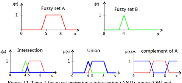
The basic fuzzy sets operations are union, intersection, and complement. Figure 12 illustrates the standard fuzzy sets operations. Fuzzy set A and fuzzy set B are two fuzzy sets defined in the universe, U. In this figure, the results of the fuzzy set operations are marked in blue. Similar with the classical Boolean set operation, the standard fuzzy set union is based on maximum operation, the standard fuzzy set intersection is based on minimum operation, and the standard fuzzy set complement is based on complement operator. The standard fuzzy union is represented by the logic OR, while the standard fuzzy intersection is represented by logic AND. Table 4 shows the mathematical operations of type-1 fuzzy set operations.
Figure 12. Type-1 fuzzy set operations: intersection (AND), union (OR) and complement.
30
Table 4. The standard operation of type-1 fuzzy sets.
Fuzzy operations Definition
Standard fuzzy intersection of set A and B
(A ∩ B)(𝑥) = min [A(𝑥), B(𝑥)] for all x 𝜖 U
Standard fuzzy union of set A and B (A ∪ B)(𝑥) = max [A(𝑥), B(𝑥)] for all x 𝜖 U Standard fuzzy complement of set A A(𝑥) = 1 − A(𝑥) for all x 𝜖 U
Besides the standard fuzzy set union, intersection, and complement, there are some customized definition of fuzzy set operation based on dependent context and application. The empirical justification of these types of operations is based on either axiomatic definition or intuitive design. The family of fuzzy union operations is known as t-connorms, while the family of fuzzy intersection operations is known as t-norms [37].
Let A, B and C be three fuzzy sets in the Universe, U. Table 5 shows the properties of fuzzy sets. The important properties for fuzzy sets are associativity, distributivity, commutativity, indempotency, identity, transitivity, involution, and De Morgan’s principles. The only properties that apply for Boolean sets but not apply for fuzzy sets are the excluded middle axioms, including the axiom of the excluded middle and the axiom of the contradiction. The following two equations express these two axioms for fuzzy sets:
Eq. (3-8) A ∪ A ̅ ≠ U
Eq. (3-9) A ∩ A ̅ ≠ ∅
31
Table 5. Properties of fuzzy sets.
Property Definition Associativity A ∪ (B ∪ C) = (A ∪ B) ∪ C A ∩ (B ∩ C) = (A ∩ B) ∩ C Distributivity A ∪ (B ∩ C) = (A ∪ B) ∩ (A ∪ C) A ∩ (B ∪ C) = (A ∩ B) ∪ (A ∩ C) Commutativity A ∪ B = B ∪ A A ∩ B = B ∩ A Indempotency A ∪ A = A A ∩ A = A Identity A ∪ Ø = A A ∩ U = A
Transitivity If A ⊆ B and B ⊆ C, then A ⊆ C
Involution
A = A
Morgan’s principles A ∩ B ̅̅̅̅̅̅̅̅ = A̅ ∪ B̅ A ∪ B
̅̅̅̅̅̅̅̅ = A̅ ∩ B̅
3.2.3. Type-1 Fuzzy Rules and Reasoning
In this section, type-1 fuzzy rules and reasoning are introduced, including fuzzy extension principal and α-cut Decomposition Theorem. The fuzzy rules and reasoning are
32
important for the arithmetic operations with fuzzy sets. Fuzzy rules and reasoning are the backbone of the fuzzy inferences, which are the key steps in the fuzzy logic modeling.
3.2.3.1. Fuzzy Relations
In addition, arithmetic operations are possible with fuzzy sets through the extension principle. The extension principle permits the fuzzification of mathematical structures based on set theory. A basic concept of fuzzy set theory provides steps to extend mathematical expression of crisp domains to fuzzy domains. Assume that 𝑓 is a function from X to Y, as defined in Eq. (3-10).
Eq. (3-10) A =µ𝐴(𝑥1) 𝑥1 + µ𝐴(𝑥2) 𝑥2 + ⋯ + µ𝐴(𝑥𝑛) 𝑥𝑛 Through the mapping 𝑓, the fuzzy set A can be expressed as a fuzzy set B as Eq. (3-11) Eq. (3-11) 𝐵 = 𝑓(𝐴) =µ𝐴(𝑥1) 𝑦1 + µ𝐴(𝑥2) 𝑦2 + ⋯ + µ𝐴(𝑥𝑛) 𝑦𝑛 𝑦𝑖 = 𝑓(𝑥𝑖)
If 𝑓 is a many-to-one mapping, which means there exists 𝑥1, 𝑥2 ∈ 𝑋, 𝑥1 ≠ 𝑥2, and
𝑓(𝑥1) = 𝑓(𝑥2) = 𝑦∗, 𝑦∗ ∈ 𝑌. In this situation, the membership function of B at 𝑦 = 𝑦∗ is the maximum of the membership function of A at 𝑥 = 𝑥1 and 𝑥 = 𝑥2, since 𝑓(𝑥) = 𝑦∗ may result from 𝑥 = 𝑥1 or 𝑥 = 𝑥2, as Eq. (3-12).
33
Besides the extension principle, arithmetic operations with fuzzy sets can be obtained through the α-cut Decomposition Theorem, which give the same results by using Zadeh’s extension principle [38].
Definition 3.7: “α-cut”
The “α-cut” of a type-1 fuzzy set A, denoted as A𝛼 , is a crisp set defined by Eq. (3-13). An example of the α-cut of a Trapezoid type-1 fuzzy set is shown in Figure 13.
Eq. (3-13) A𝛼= {𝑥 | µA(𝑥) ≥ 𝛼} = [𝑎(𝛼), 𝑏(𝛼)]
α is a value between 0 and 1.
34
Definition 3.8: Indicator function Eq. (3-14) 𝐼𝐴(𝛼)(𝑥) = {
1, ∀ 𝑥 ∈ 𝐴(𝛼) 0, ∀ 𝑥 ∉ 𝐴(𝛼)
An important application of α-cut and indicator function is that they can be used to represent a type-1 fuzzy set. The following theorem is about the representation of a type-1 fuzzy set through α-cut and indicator function.
Theorem 1 (type-1 fuzzy set Decomposition Theorem)
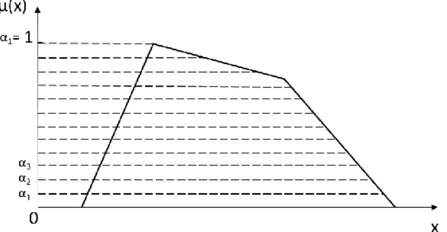
A type-1 fuzzy set can be represented through Eq. (3-15) and Eq. (3-16) [39]. An example of the type-1 fuzzy set decomposed by n α-cuts is shown in Figure 14.
Eq. (3-15) µA(𝑥|𝛼) = 𝛼𝐼𝐴(𝛼)(𝑥) Eq. (3-16) µA(𝑥) = ⋃𝛼∈[0,1] µA(𝑥|𝛼)
µA(𝑥|𝛼) is all the points of x of a specific α-cut of the type-1 fuzzy set A. ⋃ Denotes the standard union operator.
35
Figure 14. Illustration of the T1 FS Decomposition Theorem when n α-cuts are used.
3.2.3.2. Fuzzy Inference
Definition 3.9: Fuzzy If-Then Rules
A fuzzy if-then rule is presented in the form: If x is A, then y is B.
A: linguistic terms defined by fuzzy sets on the universes X, it also named premise or antecedent;
B: linguistic terms defined by fuzzy sets on the universe Y, it also named conclusion or consequent.
There are many types of fuzzy inference systems that have been used in multiple applications, among which the most widely used are Mamdani fuzzy inference system [40], Sugeno fuzzy inference system (also known as TSK fuzzy system) [41] and
36
Tsukamoto fuzzy inference system[42]. Both Mamdani and Sugeno fuzzy procedures are used in this study.
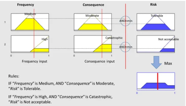
A two fuzzy inference systems are used to illustrate the Mamdami and Sugeno procedures. Three linguistic variables are used in this example. Risk: {Tolerable, Not acceptable}; Frequency: {Medium, High}; Consequence: {Moderate, Catastrophic}. The Mamdani model uses if-then rules such as:
IF “Frequency” is Medium, AND “Consequence” is Moderate, “Risk” is Tolerable.
IF “Frequency” is High, AND “Consequence” is Catastrophic, “Risk” is Not acceptable.
The connector AND can be replaced by OR in some cases, and they are calculated by the operation of intersection and union, respectively. Figure 15 is an illustration of how a two-rule Mamdani fuzzy inference system derives the overall output “Risk” when subjected to two inputs “Frequency” and “Consequence”.
37
Figure 15. Mamdani fuzzy inference system.
Figure 16 illustrates the procedure of Sugeno (TSK) fuzzy inference system derives the overall output “Risk” when subjected to two inputs “Frequency” and “Consequence”. The Sugeno model uses if-then rules such as:
IF “Frequency” is Medium, AND “Consequence” is Moderate, “Risk”=f1(frequency, consequence)
IF “Frequency” is High, AND “Consequence” is Catastrophic, “Risk”=f2(frequency, consequence)
38
Figure 16. Sugeno (TSK) fuzzy inference system.
3.2.4. Type-1 Fuzzy Modeling
Fuzzy modeling can be implemented by four steps through Matlab Fuzzy logic tool box, and the conceptual structure of modeling system is interpreted in Figure 17.
39
Step1: Fuzzification of input and output variables. Select relevant input and output variables as well as the universe of discourses for each variable. Then, determine the number of linguistic terms for each input and output variables and establish fuzzy membership functions.
Step 2: Fuzzy inference system. Choose a specific type of fuzzy inference system. Design a list of fuzzy if-then rules based on available knowledge and data (common sense, knowledge from experts, and physical laws).
Step 3: Defuzzification of the resultant fuzzy membership function. Translate the output from all fuzzy if-then rules into an understandable crisp value. There are many different types of defuzzification methods, including max membership principle, centroid method, weighted average method, mean max membership, center of sums, center of largest area, and first (or last) of maxima [37]. The most commonly used method is Centroid (COA) approach, as Eq. (3-17).
Eq. (3-17) 𝐶𝑂𝐴 =∫ 𝑥µ𝐶(𝑥)𝑑𝑥
∫ µ𝐶(𝑥)𝑑𝑥
µ𝐶(𝑥) : the resultant membership function of output.
Note: From the point of view of using all information for a decision, also the quantified uncertainty in the outcome, the defuzzification step can be regarded as a disadvantage of the method because, although the reading of a crisp value is more clear, by the defuzzification the uncertainty information is lost.
Step 4: Optimization of the whole system. Through the interview with human experts who are familiar with the target systems and more studies, parameters of
40
membership functions (MFs) can be further modified and more rules can be incorporated into the system.
3.3. Type-2 Fuzzy Logic
This section introduces the basic concepts, and basic operations for the type-2 fuzzy sets and modeling. Basically, a type-2 fuzzy set is a set in which we also have uncertainty about the membership function. A higher degree of approximation can be achieved in modeling real world problems.
3.3.1. Type-2 Fuzzy Set
In this study, type-2 fuzzy logic will also be used to modify the LOPA methodology. The concept of a type-2 fuzzy set was introduced by Zadeh in 1975 as an extension of the concept of the type-1 fuzzy set [43]. The difference between a type-1 fuzzy set and a 2 fuzzy set is that the membership grade for each element of the type-1 set is a crisp number in [0,type-1], while the membership grade of type-2 set is a fuzzy set in [0,1]. Type-1 fuzzy sets can be treated as a first-order approximation to the uncertainty in the real life, and type-2 fuzzy sets is a second-order approximation. As illustrated in Figure 18, we can get a type-2 fuzzy set by blurring a type-1 membership to the left and to the right.
41
Figure 18. Type-2 membership function as a blurred type-1 membership function [44].
Definition 3.10: A type-2 fuzzy set à is characterized by its membership function: Eq. (3-18) 𝐴̃ = ∫ ∫𝑢∈𝐽 𝜇Ã(𝑥, 𝑢)/(𝑥, 𝑢)
𝑥⊆[0,1] 𝑥∈𝑈Ã
x: the primary variable, and it has domain 𝑈Ã.
u: the secondary variable, and it has domain 𝐽𝑥 ⊆ [0,1] at each 𝑥 ∈ 𝑈Ã 𝐽𝑥: the primary membership of x, and it is defined in Eq. (3-4)
𝜇Ã(𝑥, 𝑢): the secondary membership function of Ã
To better understand the concept of type-2 fuzzy sets and the difference between type-1 fuzzy set and type-2 fuzzy set, let’s look at some examples.
Example 1. Consider the case of a type-2 fuzzy set characterized by a half circle membership function with a constant radius r, and the center is moving horizontally.
42
In this example, the membership grade µ(x) of any specific x can be a number of any possible values depends on the value of a. For example, µ(x) can be any number between 0.886 and 0.994 when x equals to 1.5, as shown in the figure 19. In this example, the membership grade of the type-2 fuzzy set is an interval. While the membership grade of a type-1 fuzzy set is a crisp value.
Figure 19. Type-2 fuzzy set example I.
Example 2. Consider the case of a fuzzy set characterized by a half circle membership function with a constant radius r, and the center is moving vertically, shown in Figure 20. Same with example 1, to a specific x value, the membership function µ(x) is an interval.
43
Figure 20. Type-2 fuzzy set example II.
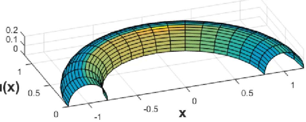
Example 3. A torus type-2 is a fuzzy set in which the membership grade of every domain point is a half circle type-1 membership function, shown in Figure 21. This example shows a more complicated case. The membership function µ(x) is three-dimensional. To a specific x value, the membership function µ(x) is a type-1 fuzzy set.
Eq. (3-21)
𝑓(𝑥, 𝑦, 𝑧) = (𝑅 − √𝑥2+ 𝑦2)2+ 𝑧2− 𝑟2; 𝑅 = 1, 𝑟 = 0.2, 𝑦 ≥ 0, 𝑧 ≥ 0 R : the distance from the center of the tube to the center of the torus; r : the radius of the tube.
44
Figure 21. Type-2 fuzzy logic example III.
3.3.2. Interval Type-2 Fuzzy Set
Interval type-2 fuzzy set is one in which the membership grade of every domain point is a crisp set whose domain is some interval within [0,1]. Both figure 19 and figure 20 are interval 2 fuzzy sets. Interval 2 fuzzy set is a simplified version of type-2 fuzzy set. The membership function to a specific x value is a crisp set, whose domain is an interval between 0 and 1. The fuzzy sets in example 1 and example 2 are interval type-2 fuzzy sets. Figure type-2type-2 shows the comparison of a type-1 Trapezoid fuzzy set and an interval type-2 Trapezoid fuzzy set.
45
Figure 22. (a) Type-1 fuzzy set; (b) Interval type-2 fuzzy set.
An interval type-2 fuzzy set can be treated as a region between two type-1 fuzzy sets. As shown in the figure 22(b), the interval type-2 fuzzy set 𝑩̃ can be treated as the region between the upper membership function 𝐵 ̅ and the lower membership function. In other words, the upper membership function 𝐵 ̅is the upper boundary of an interval type-2 fuzzy membership function, and the lower membership function Ḇ is the lower boundary of an interval type-2 fuzzy membership function. The green region in between is named the footprint of uncertainty (FOU). Mathematically, an interval type-2 fuzzy is the union of type-1 fuzzy membership function [45].
In example 2, the upper membership function is described in Eq. (3-22) and the lower membership function is described in Eq. (3-23). And the region in between 𝐵 ̅and
𝐵 is the FOU. With the definition of FOU, Eq. (3-24) describes a very compact way to represent an interval type-2 fuzzy set.
Eq. (3-22) 𝐵 ̅ = √1 − (𝑥 − 1)2 ; 𝑏 𝜖 [0 , 0.4], 𝐵 ̅ ≥ 0 Eq. (3-23) 𝐵 = √1 − (𝑥 − 1)2− 0.4 ; 𝑏 𝜖 [0 , 0.4], Ḇ ≥ 0 Eq. (3-24) 𝐵̃ = 1/𝐹𝑂𝑈(𝐵̃)
46
1/𝐹𝑂𝑈(𝐵̃): The division sign is not the mathematical operation of division. It means that the secondary grade equals to 1 for all elements of FOU for set 𝐵̃.
3.3.3. Basic Operations
In this section we describe the operation of the interval type-2 fuzzy sets, including union, intersection and complement.
Figure 23. Standard interval type-2 fuzzy sets operations (a). Interval type-2 fuzzy set 𝐴̃
and 𝐵̃. (b). Standard union of 𝐴̃ and 𝐵̃. (c). Standard intersection of 𝐴̃ and 𝐵̃.
Similar with standard type-1 fuzzy logic operation, interval type-2 fuzzy set union is based on maximum operation, interval type fuzzy set intersection is based on minimum operation, and interval type-2 fuzzy complement is based on complement operator. The
47
standard fuzzy union is represented by the logic OR, while the standard fuzzy intersection is represented by logic AND. Figure 23 shows the set operations of two interval type-2 fuzzy sets 𝑨̃ and 𝑩̃. Table 6 shows the mathematical definition of the interval type-2 fuzzy set operations.
Table 6. The standard operation of type-2 fuzzy sets.
Fuzzy operations Definition
Standard fuzzy intersection of set 𝑨̃ and𝑩̃ (𝑨̃ ∩ 𝑩̃ )(𝑥) = min [𝑨̃ (𝑥), 𝑩̃ (𝑥)] for all x 𝜖 X
Standard fuzzy union of set 𝐴̅ and 𝑩̃ (𝑨̃ ∪ 𝑩̃ )(𝑥) = max [𝑨̃(𝑥), 𝑩̃ (𝑥)] for all x 𝜖 X
Standard fuzzy complement of set 𝑨̃ 𝑨̃(𝑥) = 1 − 𝑨̃(𝑥) for all x 𝜖 X
3.3.4. Interval Type-2 Fuzzy Reasoning
Theorem 2: Representation Theorem for an interval type-2 fuzzy set[46]
This theorem allows an interval type-2 fuzzy sets be represented in term of type-1 fuzzy sets. Assume x is the primary variable of an interval type-2 fuzzy set Ã, and it is sampled at N values, x1, x2, …, xN. µi is the primary memberships at each of x values, and it is sampled in Mi values, ui1, ui2, … uiM. Let 𝐴𝑒𝑗 denote the jth embedded type-1 fuzzy set for
48 Eq. (3-25) 𝐹𝑂𝑈(Ã) = ⋃ 𝐴𝑒𝑗 𝑛𝐴 𝑗=1 = {𝐴(𝑥), … , 𝐴(𝑥)} ≡ [𝐴(𝑥), 𝐴(𝑥)]
𝑛𝐴 : the total number of M.
𝐴𝑒𝑗 : the jth embedded type-1 fuzzy set for Ã.
Same with type-1 fuzzy set, there are different types of fuzzy inference systems for type-2 fuzzy modeling, including Mamdani inference and Sugeno (TSK) inference. The consequent of a Mamdani rule is a fuzzy set, while the consequent of a Sugeno rule is a function.
3.3.5. Interval Type-2 Fuzzy Modeling
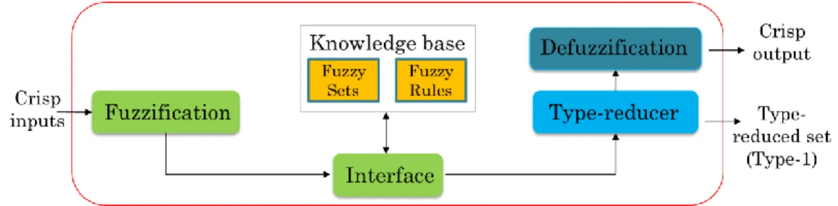
In the 2 fuzzy system, as illustrated in Figure 24, there is a step called type-reducer before the final defuzzification. The final results of type-2 fuzzy membership function need to be reduced to type-1 fuzzy membership function, then defuzzified to a crisp value.
49
Figure 24. The structure of type-2 fuzzy logic system.
Step1: Fuzzification of input and output variables. (If Sugeno fuzzy inference is used, only fuzzification of input variables is needed. The output variables are then determined by a function of input variables.) Select relevant input and output variables as well as the universe of discourses for each variable. Then, determine the number of linguistic terms for each input and output variables and establish fuzzy membership functions.
Step 2: Fuzzy inference system. Choose a specific type of fuzzy inference system. Design a list of fuzzy if-then rules based on available knowledge and data (common sense, knowledge from experts, and physical laws).
The following shows an example of a Sugeno rulebase of an Interval type-2 fuzzy set consisting of N rules assuming the following forms:
Rn: IF x1 is 𝑋̃1𝑛 and … and xI is 𝑋̃𝐼𝑛, THEN y is Yn n = 1, 2, … N Rn: nth rule
𝑋̃𝑖𝑛: interval type-2 fuzzy set
50
Assume the input vector is 𝑥′= (𝑥1′, 𝑥2′, … , 𝑥𝐼′). Then the firing interval of the nth rule, 𝐹𝑛(𝑥′), can be calculated through the following function:
Eq. (3-26) 𝐹𝑛(𝑥′) = [𝜇 𝑋1𝑛(𝑥1 ′) × … × 𝜇 𝑋𝐼𝑛(𝑥𝐼 ′), 𝜇 𝑋1 𝑛(𝑥1′) × … × 𝜇 𝑋𝐼 𝑛(𝑥𝐼′)] ≡ [𝑓𝑛, 𝑓 𝑛 ] 𝑋̃𝑖𝑛 = [𝜇𝑋 𝑖𝑛(𝑥𝑖 ′), 𝜇 𝑋𝑖
𝑛(𝑥𝑖′)]: the membership function 𝑥𝑖′
Step 3: Type-reducer and defuzzification of the resultant fuzzy membership function. Type-reduction then is performed to combine 𝐹𝑛(𝑥′) and the corresponding rule consequents. There are different methods, and the most widely used method is the center-of-sets type-reducer [47]: Eq. (3-27) 𝑌𝑐𝑜𝑠(𝑥′) = ⋃ ∑𝑁𝑛=1𝑓𝑛𝑦𝑛 ∑𝑁 𝑓𝑛 𝑛=1 𝑓𝑛𝜖 𝐹𝑛(𝑥′) 𝑦𝑛𝜖𝑌𝑛 = [𝑦𝑙, 𝑦𝑟]
KM algorithm [48] can be used to calculate 𝑦𝑙 and 𝑦𝑟. The defuzzified output can be calculated through the following equation:
Eq. (3-28) 𝑦 = 𝑦𝑙+𝑦𝑟
2
Step 4: Optimization of the whole system. Through the interview with human experts who are familiar with the target systems and more studies, parameters of membership functions (MFs) can be further modified and more rules can be incorporated into the system.
51
4. A PROBABILISTIC AND FUZZY LOGIC HYBRID APPROACH *
This section describes a fuzzy logic and probabilistic hybrid approach that was developed to determine the mean value and to quantify the uncertainty of frequency of an initiating event and the probabilities of failure on demand (PFD) of independent protection layers (IPLs). It is based on the available data and expert judgment. The method was applied to a distillation system with a capacity to distill 40 tons of flammable n-hexane.
4.1. Uncertainty Sources in Failure Rate
Layer of protection analysis (LOPA) provides a simplified and less precise method to assess the effectiveness of protection layers and the residual risk of an incident scenario. The outcome failure frequency and consequence of that residual risk are intended to be conservative. This makes the risk in a conservative approach usually overestimated.
The failure rate consists of the frequency of an initiating event and the probabilities of failure on demand (PFD) of independent protection layers (IPLs). They are related with the frequency part of the risk. Two aspects are investigated in this part. First aspect is the sources of uncertainty in failure rate. Second aspect is the representation of uncertainty in failure rate data.
* Part of this section is reprinted with permission from “A fuzzy logic and probabilistic hybrid approach to quantify the uncertainty in layer of protection analysis” by Yizhi Hong, Hans J. Pasman, Sonny Sachdeva, Adam S. Markowski, and M. Sam Mannan, 2016. Journal of Loss Prevention in the Process Industries 43, Copyright 2016 by Elsevier.
52
Uncertainty exists in the failure rate data. Generally speaking, if there are more data in the database, and all the data are scientifically collected and analyzed, the data will be more accurate, i.e., there is less uncertainty in the database. Moreover, the sources of the data can also affect the amount of uncertainty. There are two types of database, including generic database and plant-specific database. Table 7 shows the definition, advantages and disadvantages of generic database and plant-specific data. Typical generic databases are available at the Center for Chemical Process Safety (CCPS) [49] and the Offshore Reliability Data Handbook (OREDA) [50]. Compared to generate database, plant-specific data are first-hand data, and it can better reflect the actual situations of the process and equipment. The ideal method to eliminate uncertainty is collecting enough plant-specific data. However, an extensive data collection system for a plant is much time and money consuming and in practice not realizable. Generic databases, which provide a much larger pool of data, are less specific and have less detail. The environmental conditions and operating conditions, the maintenance policy, and the definition and boundary of the investigating instruments can be different from those of the instruments in the generic databases. In these situations, using generic databases could increase the uncertainty. Moreover, expert knowledge is used in some situations when no data are available.
53
Table 7. Comparison of generic databases and plant-specific failure data.
Generic databases plant-specific failure data
Def. Data from a variety of plants and industries
Failure data from the on-site plant
Pros Provide a much larger pool of data Reflect the plant's process, environment, maintenance practices, and operation of equipment
Cons Less specific and detailed Data collection is very difficult, and an extensive data collection system is expensive
In conventional LOPA, single point values or the upper bounds of intervals of failure rates are derived from historical data or literature, and there is no uncertainty information in a point value. The expression of the data in this way does not take the uncertainty into account.
4.2. Relevant Literature Review and Gap Identification
Markowski and Mannan [10] developed a fuzzy LOPA (fLOPA) approach for risk assessment of transportation of flammable substances in long pipelines. The risk value calculated by fLOPA shows a more accurate result than those given by conventional LOPA. Khalil et al. [51] developed a cascaded-fuzzy LOPA risk assessment model with
![Figure 2. Spectrum of tools for risk-based decision making [28].](https://thumb-us.123doks.com/thumbv2/123dok_us/837639.2606465/20.918.185.763.130.462/figure-spectrum-tools-risk-based-decision-making.webp)
![Figure 4. Layers of protection for a possible incident [28].](https://thumb-us.123doks.com/thumbv2/123dok_us/837639.2606465/26.918.267.679.143.617/figure-layers-protection-possible-incident.webp)
![Figure 5. The process life cycle showing where LOPA is typically used [2].](https://thumb-us.123doks.com/thumbv2/123dok_us/837639.2606465/27.918.205.749.501.750/figure-process-life-cycle-showing-lopa-typically-used.webp)