Soverign lending spreads

Sovereign Lending Spreads

by

Peter Benczur

MASSACHRSETS SI-OTECHNOLOGY.

MOR 16

O1

LIBRARIES

Submitted to the Department of Economics

in partial fulfillment of the requirements for the degree of

Doctor of Philosophy

at the

MASSACHUSETTS INSTITUTE OF TECHNOLOGY

February 2001

( Peter Benczur, MMI. All rights reserved.

The author hereby grants to MIT permission to reproduce and distribute publicly

paper and electronic copies of this thesis document in whole or in part.

Author

...

...

Department of Economics

December 18, 2000

Certified

by ...

,

Certified

by..., ...

...

...

Yr0|~~

~Daron

Acemoglu

Professor of Economics

Thesis Supervisor

... ... ... o .. ... . .

Rudiger Dornbusch

Ford International Professor of Economics

Thesis Supervisor

Accepted by ...

Peter Temin

Elisha Gray II Professor of Economics

Chairman, Department Committee on Graduate Students

Sovereign Lending Spreads

by

Peter Benczur

Submitted to the Department of Economics

on December 18, 2000, in partial fulfillment of the

requirements for the degree of

Doctor of Philosophy

Abstract

This thesis studies the determinants of sovereign lending spreads. The objective of the first chapter is to identify and disentangle various risks embodied in foreign currency

denom-inated sovereign bond spreads. Its empirical approach tries to attribute the explanatory

power of country fundamentals in a spread equation to their predictive power for default

and illiquidity risk. For this, I incorporate rational expectation predictions into the spreads

and propose an IV estimation method. The overidentification test offers a test whether

the spread can be explained by predicted risk probabilities. Applying this approach to

de-veloping country bond data from 1975 to 1995, I find that the non-structural explanatory

power of fundamentals can be completely attributed to their influence on predicted risk

probabilities.

The second chapter takes a broader view across all public sovereign lending. Data from the World Bank suggests that the average spread on all forms of borrowing by developing countries is smaller than for top-rated US corporate bonds. After documenting these facts (with particular care for resolving data problems), the analysis looks behind the averages. Once identifying various sub-types of borrowing, I find that official and other private lending (trade-related) are the main source of the low average spreads. Bond and commercial bank lending shows reasonable spreads. Unlike other and official, bond and bank lending move nearly one in one with world interest rates. All types of private lending significantly differ

from each other in the way they incorporate country fundamentals.

The third chapter offers a potential source of liquidity risk in bond markets: in a Diamond-Dybvig type model, where agents face a risk of becoming more risk-averse early consumers, changes in the speed of public learning about default risk may increase bond spreads, and decrease investor welfare. This effect operates through a link between future price volatility and current prices: increased expected future price volatility leads to lower prices today.

Thesis Supervisor: Daron Acemoglu Title: Professor of Economics

Thesis Supervisor: Rudiger Dornbusch

Acknowledgments

In the preparation of this dissertation, I have benefited immeasurably from the advice,

patience, friendship, and wisdom of a number of people.

My foremost thanks to Daron Acemoglu, for his rigorous comments, helpful advice, and pushing me to sharpen my half-made products into final projects. Jaume Ventura helped enormously to transform my vague ideas into a concrete and really interesting research agenda. Rudi Dornbusch offered the purgatory of International Breakfasts. Ricardo Ca-ballero's classes convinced me to do international macroeconomics as my primary field, and discussions with him always made me focus on finding the question first. Last but not least in this row, I thank Olivier Blanchard, Francesco Giavazzi, Roberto Rigobon, and all participants of the International Breakfast and Macro Lunch, for being an endless source of discussions, sound advice and ideas.

I am also indebted to all my fellow students, who shaped much of my learning, working and living environment: D)irk (and Ruth), Petya, Kobi, Markus, Botond, Alejandro, Eric and Fernando. Apologies to all whom I accidentally left out from the list.

No research would have been possible without the supportive atmosphere of friends.

I wish to thank all my roommates: Andras, Szabolcs, Peter, Attila and Gyula; the MIT

Isshinryu Club and the Wrldwide Hungarian Conspiracy (in Boston and in Budapest).

I thank the Soros Foundation for partial financial support, and the Department of

Economics for its fellowship and teaching assistantship awards.

Finally, my deepest gratitude to my family and Eszter. Their permanent support is ever

appreciated.

Contents

Introduction

1 Decomposing sovereign bond risks

1.1 Introduction .

...

1.2 A simple model establishing a link between current and expected future prices

1.3 The setup of the empirical analysis ...

1.3.1 Variables, data sources. 1.3.2 Main specification. 1.4 Main results .

1.4.1 First pass:: only default risk ...

1.4.2 Identification and generalization of the metho,

1.4.3 Illiquidity risk .

1.5 Robustness checks of the results ...

1.5.1 Different left hand side variable . . . .

1.5.2 Different estimation techniques ...

1.5.3 Varying the event indicators ...

1.5.4 Country and time effects ...

1.6 Summary and conclusions ... 1.7 Appendix ...

1.7.1 Multiple equilibria in the model ...

1.7.2 Deriving identification for the two event case References .

... . .22

... . .22

... . .23

... .. ..24

... .. . ... . .. . .24

d ...

.

31

... . .36

... . . . . .. . .. . .40

... . .40

... . .41

. .. . . . .. . .42

... . .44

... . .47

...

.50

. . . ... 50 ... . .. 51 . . . ... .52

2 The composition of sovereign debt: a description

2.1 The behavior of average borrowing rates ...

54 54 9 11 11 17

2.1.1 Borrowing rates are very low ...

2.1.2 Borrowing rates respond too little to world interest

2.2 Relation to the literature ...

2.3 The data:

2.3.1 Ecoi 2.3.2 Deb 2.4 The weight,

2.5 Validation (

2.6 Main result 2.6.1 Diffi 2.6.2 Diffi 2.7 Robustness 2.7.1 Usir 2.7.2 Diffi 2.8 Alternative 2.9 Conclusion 2.10 Appendix 2.10.1 The 2.10.2 The 2.10.3 Reg: References . . .

sources;, problems and remedies ... nomic indicators of countries ...

t data ...

ed estimation ...

of the Data ...

s . . . .

rences by lending types ... erences by income groups ...

checks

...

ig different compositions ...

brent methods, grouping by regions and

interpretations

...

s . . . .. . . . .

right hand side variables (factors) . . .

disbursement-commitment correction

ression results ... ... ... . . .. . .. . .. . .. . .. . .. . .. .

time

. . . . .. . .. . .. pe

rates

58

... . .61

... ..62

... ..62

... ..63

... . .66

... ..69

... . .72

... . .72

... ..78

... ..83

... . .83

riods ...

84

... . .84

... . .89

... . .. 91 ... . .. 91

... . .93

... . .94

... . .96

3 Learning, noise traders, the volatility and the level

3.1 Introduction .

3.2 The model .

3.2.1 Ingredients.

3.2.2 Solving the model - slow learning case .... 3.2.3 The fast learning case ...

3.3 Results .

...

3.3.1 Comparing slow and fast learning ... 3.3.2 A continuous version of the speed of learning 3.4 Conclusions ...

of bond spreads

. . . .. .. . . ... . . . . ... . . . · . . . . . . . . . . . . . . . . . . . . . . . . . . .

97

97 102 102 103 105 107 107 116 120 54

List of Figures

2-1 Interest rates and spreads ...

55

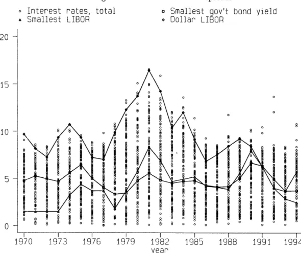
2-2 Interest rates and spreads ...

57

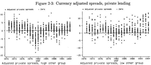
2-3 Currency adjusted spreads, private lending ...

58

2-4 Data from World Debt Tables vs Borrowing in International Capital Markets 71 2-5 Estimated spreads; using flow and disbursements weights ... 78

2-6 Lending spreads by income groups ... .... 81

2-7 Estimated spreads of private lending types, by income groups ... 82

2-8 Evolution of the other-official ratio and lagged world interest rates ... 86

2-9 Private debt of Iran, 1980-1994 ... 89

List of Tables

1.1 Describing bond yields ...

1.2 The prediction equations ...

1.3 Regression results: only default risk considered . . .

1.4 Main results . . . .

1.5 Different left hand side variable ... 1.6 Different estimation techniques ... 1.7 Country effects.

1.8 Time effects.

2.1 Results for total, official and private lending ...

2.2 Comparing the weighted and non-weighted estimates

2.3 Bank lending estimates .

2.4 Baseline costs of lending: decomposition by types . . 2.5 Differences by types of lending ...

2.6 Different types of lending: quantity responses .... 2.7 Reduced form estimates: using "flow" composition .

3.1 Utility and price comparison ...

26 28 30 ... .. . .. . . .. . .37 .. ... . . . .. . .40 . . . .. . . . ... .41

...

.45

... . .46

. . . ... .59

... .. . 68

...

.70

... .. 73 ... .. 75 . . . ... .. .. 77

...

.95

113

Introduction

This thesis studies the determinants of sovereign lending spreads. The first chapter focuses on bonds: its objective is to identify and disentangle various risks (in particular, default and liquidity risk) embodied in foreign currency denominated sovereign bond spreads. First I present; a simple model of pure liquidity risk, where risk-neutral investors trade a perfectly safe bond at a positive spread relative to a benchmark interest rate. This effect is driven by a link between current and predicted future, pre-maturity price fluctuations.

The main focus is on the empirical approach, which tries to attribute the explanatory

power of country fundamentals in a spread equation to their predictive power for default

and illiquidity risk. For this, I incorporate rational expectation predictions into the spreads

and propose an IV estimation method. The overidentification test then offers a ready test

whether the spread can be explained by predicted risk probabilities. Applying this approach

to developing country bond data from 1975 to 1995, I find that the non-structural

explana-tory power of fundamentals can be completely attributed to their influence on predicted

risk probabilities.

On average, default risk is 27% of the spread; for a 10 percentage points increase in predicted default probability, the spread rises by 31.5 basis points. Illiquidity, which is captured by future price volatility, gives an additional 27%; for an increase of variance by 10 (the sample average is about 50-60), the spread goes up by 26 basis points. The remaining 46% is attributed to adjustments, country effects and aggregate illiquidity (captured by lagged spreads and US interest rates).

The second chapter takes a broader view across all public and publicly guaranteed sovereign lending. In contrast to all expectations, data from the World Bank suggests that the average spread on all forms of borrowing by developing countries is smaller than for top-rated US corporate bonds. Part of this phenomenon is due to official lending, which is

extremely cheap, but even average private lending spreads are near or below zero.

The chapter documents these facts (with particular care for resolving various data

prob-lems), and then looks behind the averages. Once identifying various sub-types of borrowing, I find that official and other private lending (trade-related, or at least more firm-level lend-ing) are the main source of the surprisingly low average spreads: these two types of lending

react very little to movements in international interest rates, which - together with a not

sufficiently large constant term - makes these types of loans very cheap. This also gives an

"interest rate smoothing" result for official and other private lending.

Bond and commercial bank lending shows reasonable spreads, and both move nearly one in one with world interest rates. All types of private lending significantly differ from

each other in the way they incorporate country-specific or worldwide economic conditions.

Moreover, low-income countries actively change their disbursement portfolio in response to

world interest rates, which leads to "interest rate smoothing" of commercial bank lending

rates as well.

The third chapter returns to the issue of liquidity in bond markets. According to the first

chapter and various other studies, sovereign bond spreads often deviate from any "sensible" perception of default risk. It is usually attributed to behavioral effects (overreaction) or liquidity. The former explanation imposes some irrationality or bounded rationality on investors; while the latter usually relies on some informational asymmetry or thin markets.

The chapter presents a different source of liquidity risk: in a Diamond-Dybvig type model, where agents face a liquidity risk (becoming more risk-averse early consumers), changes in the speed of public learning about default risk may increase bond spreads. This effect will operate through a link between future price volatility and current price levels: increased expected future price volatility (a volatility effect) leads to lower prices today (a level effect). Under reasonable parameter values, accelerated information revelation may increase spreads by 50%.

I also compare the welfare of the issuer and investors under different speeds of learning: revealing information may be good or bad for the issuer (issue prices may increase or decrease), and also for the investors (ex ante utility might be higher or lower).

Chapter 1

Decomposing sovereign bond risks

1.1 Introduction

It is a standard notion to view bond prices as the market's assessment of the riskiness of the issuer. Aside from whether or not market participants are right, it is not clear, however, what this risk is. It might reflect the inability to pay (default risk), or a situation when

the investor needs to sell the bond before maturity and the price happens to be low at

that point (illiquidity risk). This later event might be restricted to one particular (type) of bond, in which case it is more idiosyncratic (thus it can be diversified), or to the majority of bonds, which is a situation of systemic illiquidity.

Bonds are also subject to interest rate risk: investors are committing their money

long-term to a fixed nominal interest rate, and if the short-long-term rate goes up, they are worse-off

than by investing in short-term bonds from period to period. The nominal part can be

eliminated by indexed bonds, but a real interest rate risk may still be present. Finally, if

the bonds are paying their return in a currency different from the one investors need for consumption (or in which they have to repay what was borrowed), then investors are facing an exchange rate risk as well.

Reputation, political or strategic elements may also influence borrowing terms of sov-ereigns (see Obstfeld and Rogoff (1986) [1] as a survey): in the case of bonds, fortunately, with relatively many and small investors buying the bonds, such one-to-one relationships are much less present. Therefore, I assume that bond prices reflect non-strategic and predictable risks only.

In order to concentrate on illiquidity risk, about which much less is known,1 I will focus on spreads of foreign currency (usually US dollar) denominated sovereign bonds. By

being foreign currency denominated, these bonds substantially reduce the exchange rate

component: the dollar-deutschemark rate might still fluctuate but to a smaller degree, and

much better forward markets are available to offset the effect of such fluctuations.

Working with spreads relative to similar maturity and currency-denominated govern-ment bonds (US Treasuries, German Governgovern-ment Bonds etc.), I also nullify most of the interest rate risk: in principle, investors can go short in those nearly riskless bonds and use their proceedings to buy, say, Latin-American more risky. This spread, therefore, should be

mostly independent from interest rate movements.

The objective of the chapter will be to separate default and illiquidity risk, by using

data on sovereign bond issues and default behavior of several developing countries. In

doing this, I will basically stay within the framework of risk-neutral investors with rational

expectations: I assume that the price (or rather: the spread) depends on the expected value of certain risk events (losses).

From a pure forecasting or descriptive viewpoint, it would be sufficient to learn how fundamentals of a borrower (in my case: of a sovereign country) influence the spread it has to pay on its bond issues, as it is done in various studies.2 Then a country can aim at better average terms of borrowing by improving these fundamentals. As there are always more fundamentals than what a particular specification contains, and many events or simply words of mouth can play a role but will not be captured by a researcher, one can never be safe about the reason why that specific fundamental is having this size of an effect, or whether it is reasonable or rational to have such an effect at all.

It is thus instructive to attribute these influences by fundamentals to movements in

perceived probabilities of the risks incorporated into spreads. For that, a structural setup

is necessary: risk probabilities are predicted by fundamentals, then bond spreads are de-termined by predicted probabilities. Spreads will still be influenced by fundamentals, but we will have a clearer sense of why: because they help to predict risk probabilities. Also,

'There are some theoretical papers, like Grossman and Miller (1988)[2]; and empirical contributions, but

the latter mostly concentrate on US Treasuries. For example, Redding 1999 [3], Amihud and Mendelson (1991) [4], Bradley (1991) [5] and Hirtle (1988) [6] See the third chapter for a more detailed discussion.

2

Among many others: Edwards (1986) [7], Stone (1991) [8], Ozler (1993) [9]. A different but still similar

article is in Standard and Poor's CreditWeek[10]: it explains how credit ratings, which are closely related to predicted but not necessarily to perceived risk, are responsive to country fundamentals.

this approach has the ability of gauging the relative size and importance of different risk

factors.

My approach is thus reminiscent of well-known practices for testing rational expectations (e.g. Mishkin (1983) [11], Attfield, Demery and Duck (1985) [12]). There the usual setup is as follows.3 One variable (say X) depends on the predicted value of a (potentially vector) variable Y:

Xt = a + PE[YtlZt] + vt

(1.1)

where Zt is the information available for predicting Yt (usually, it has time t-1 variables).

So one specifies a prediction (conditional expectation) equation

Yt =

f(r,

Zt) + et

(1.2)

and rewrites (1.1) as

Xt = a + of (r, Zt) + vt.

(1.3)

Then equations (1.2) and (1.3) can be estimated by some full information and in general

nonlinear method, mostly by GMM.

The reduced form of (1.3) is

Xt =

g(Zt)

+

t.

(1.4)

It describes how Xt is influenced by past information (Zt). Now suppose that some theory predicts that all the influence of Zt should come through the predicted value of E[YtlZt]

(specification (1.1). Then the structural form (1.3) rewrites the reduced form (1.4) as

g(Zt) =

+

f(zt,r).

This gives a straightforward test whether the structural form is really a good

reinterpreta-tion of the reduced from: estimating (1.2) and (1.4) simultaneously, and then testing the

3_{Since prices should incorporate all the available information, I can drop the otherwise standard}

restriction

g(Zt)

=

a +

Pf

(Zt, r).

I will follow a similar but importantly different approach: instead of using any specific functional form for f, then estimating the two equations simultaneously (full information)

and testing a nonlinear overidentification hypothesis, I will estimate

Xt = a + Yt +

A t

(1.5)

directly. Here the error term is At = vt +f (f(r, Zt) - Yt) = vt + Bet, which is not orthogonal to Yt = f(r, Zt) + Et, but orthogonal to Zt. Moreover, Yt is correlated with Zt, so I can estimate (1.5) by using 2Zt as instruments.4 _{I will elaborate this idea in more details in}

Subsection 1.4.2.

Here the overidentification test means checking if the residuals Xt -

a

-

/3Yt

are

orthog-onal to Zt: Under the null (all instruments are valid), the estimates are consistent, so the

residuals

a-a

a+

vt +

E[lZt]

- Yt = a -

a

+ vt +

(E[YtlZt]

- Yt) -

) Yt

should be orthogonal to Zt, since

&

- a -- O,

/

-

>--

0,

t I Zt, and E[YtlZt] - Yt I

Zt. The last term suggests that it is crucial that the market uses the right (rational)

expectations: without that assumption, the prediction error E[YtlZt] - Yt is in general non-orthogonal to the predictors, and overidentification fails. It also fails if the endogenous right hand side variable Yt is not the true event or not the only event the market was using. In general, I will assume rational expectations, and attribute the failure of overidentification to the inappropriate choice (or insufficient number) of events.

The previous nonlinear test would become identical to this simple test if one restricts

the functions f and g to be linear. Then I would get a linear reduced form

Xt = a' + r'Zt + vt

Yt =

a"ll

+ r"Zt + Et,

4

and the structural form would impose the restrictions

a

= a

+

pa"

andr' =

ir".

However, as the argument shows, testing the orthogonality of the residuals and the

instru-ments is a valid overidentification test even in a nonlinear setup: the only linearity I need is that Xt is influenced linearly by the predicted value of Yt (in (1.1)), but (1.2), the prediction

itself does not have to be linear. This makes this method readily applicable in many other

asset pricing frameworks (for example, estimating an uncovered interest parity condition).

The major difficulty of the approach in general is that one needs data on Yt, that is,

the actual realizations of the predicted event. If it were a standard economic variable, like

future GDP, then we (the econometrician) would indeed observe it a year later - so when

I run (1.5) on historical (at least 2-years old) data, then I already have the data which the

market only predicted at time t.

With default observations for bonds, the situation is not that simple: hardly any

sovereign bond defaults happened since the 70s (which is the beginning of my sample pe-riod).5 There were, however, much more frequent arrears, reschedulings or even defaults (debt relieves) on bank loans. As a working assumption, I will treat all defaults equally, so

even though an actual observation is not a bond default, but that will be used for the bond

default prediction equation.6

The illiquidity risk is even less clear-cut: actual trade quantity data is rarely available, so there is no other signal for liquidity than the price of the bond itself, but that also captures default risk and many other things. My main measure for illiquidity will be the sample variance of the spread from any given year on (for 3 years, 5 years, or to the end of

my sample): the interpretation is that volatile prices indicate that the bond is hard to sell

for a secure price, so it is less liquid, there is a potential loss if one is forced to sell at an arbitrary moment. As a whole, this measure will perform its role surprisingly well.

This illiquidity indicator tries to capture an effect of expected pre-maturity prices on

current prices. To the degree that price fluctuations are disjoint from predicted default risk, it means that this illiquidity variable should be significant exactly when investors face

5

See for example [14] as a reference.

6

An extreme view could be that if there are almost no bond defaults, then the predicted risk is nearly zero, thus there is no default risk in bonds.

the chance of having to sell before maturity and they incorporate a potential loss due to

low prices into their current pricing decision. Note that this is an effect of "interim" price fluctuations, and it does not come from the variance of the payoffs at maturity. Hence, even with risk-averse investors, this variance is not just a standard risk-aversion component, but it does capture an illiquidity aspect. To make this point even more transparent, I will for-mulate a model in which risk-neutral investors will trade a perfectly safe bond at a positive

spread relative to a benchmark interest rate. In the third chapter, I will pick up the same

issue, and develop a still simple but more interesting model, where the speed of

informa-tion revelainforma-tion influences future (pre-maturity) price movements, and those fluctuainforma-tions in

general decrease current (issue) prices.

With these less than perfect choices for the realizations of the risk indicators, if the true

events are different, then the predicting variables Zt might be catching up the difference

E[YttrueZt] - E[Ytch°senIZt], and thus the overidentification test of (1.5) fails. A rejection

could also be due to non-rational market expectations - and these two possibilities are

in-distinguishable even theoretically. Therefore, I will attribute any rejection to adjustments for the events (or to the presence of further relevant risks) and not to irrational expecta-tions.7 Of course, with the full (vector) yttrue observed, the overidentification would test

the rationality of expectations.

Let me briefly summarize the main findings. In the theoretical part of the chapter, I show

that a combination of future price volatility and an exogenous chance of early liquidation

leads to a risk premium on bonds with more volatility. In the more important, empirical

part, I find that the influence of fundamentals on bond spreads can' be completely attributed

to their effect through predicted risks. When including at least two risk indicators ( default,

and arrears or price volatility) and the US interest rate, or any single risk indicator, the US

interest rate and an adjustment term (lagged left hand side variable), the overidentification

test almost always accepts. Using the default indicator of any kind of repayment troubles,

overidentification accepts even without the lagged spread.

With the specification including default, price volatility, US interest rates and the

ad-7

With the US bond rate and the lagged value of the spread included in the right hand side of (1.5), I will

rarely encounter rejections of the overidentification: although it might be due to low power of those test, but I take it as a signal that my events are not so off the truth . For example, bondholders fear any kind of default, even if it is restricted to bank loans, and that fear enters prices as default risk. Price volatility

contributes as a second source of risk, related to bond-specific liquidity. I view the US bond rate as some

justment term, I find that default risk, which is captured by predicted loan and not just bond default risk, is on average 27% of the spread. Illiquidity risk, captured by predicted volatility of bond prices, constitutes an additional 27%. The other 46% of the spread is . made up by the lagged value of the spread, the US rate (which influences the spread itself)

and the constant. I interpret this 46% partly as an adjustment term reflecting some extra

information known to investors (relative to the econometrician), and partly as a notion of aggregate illiquidity. Finally, I check the robustness of the result with respect to many alternative specifications, and my findings pass these tests.

The chapter is organized as follows. The next section sketches a model to access "pure" illiquidity risk. Section 1.3 summarizes my data and the basic empirical specification I am using. Section 1.4 presents and discusses the main findings: The first part tries to explain bond spreads only by default risk. Then the method is generalized to allow for more than

one event, non-linear prediction equations and extra information available for the market.

This method yields more successful description of bond spreads, the robustness of which is tested in Section 1.5. The last section concludes and points to some possible future research

directions. Some skipped details are then presented in the Appendix.

1.2 A simple model establishing a link between current and

expected future prices

For a given (sovereign) bond, there is a mass 1 of investors holding that asset. Each of them is having 1 unit. At each point in time, a fraction A of the investors suffers a liquidity shock

and must liquidate her bond. The main assumption is that the potential buyers of the bond

have some cost of shifting their investments from other sources to this bond - which gives a slope to demand, plus they also face the same future potential liquidity shock.8

A (potentially) random fraction (1 - pt)A investors are to be found without any transfer costs (only the future liquidity shock as threat). They can be thought as big, institutional investors, who do not have to pay transaction costs, while small investors do.9 Assume that

8_{Grossman and Miller (1988) [2] also uses an imperfect market structure to capture liquidity. There,}

however, the cost falls on sellers, in the form of not necessarily finding the right buyer at the right time. In the third chapter, buyers face no cost of portfolio adjustments, but the price will fluctuate due to extra

information (learning). With more risk-averse early than late consumers, this will lead to a fall in issue prices.

.t is coming from an iid process.l °0 The important thing is to have a fluctuating mass of

investors with zero cost, thus introducing a variation in the cost level of the marginal buyer.

The bond is paying a per period interest (coupon) of R forever, R being equal to the

discount rate. There exists a similar, perfectly safe bond with coupon R, for which - 0. Its price is thus identically 1. By this assumption, I exogenously choose one market to be

perfectly liquid and the other to be less than perfectly liquid. Thinking about the market

for US Treasury Bonds versus developing country sovereign bonds, it looks reasonable to assume such an exogenous difference.

Consider holding one unit of the sovereign bond. Then the discounted value of your flow of returns is the following::

R

Ap(l

1

)

1-A

R +AP(2)

1-A

---

1+R

1+R

R+R

1 +R

1+R

Taking expectations:

R

AEp(it)

1--A

EX=

+

+ +R EX

REX + AEp(p)

EX-Suppose you are an investor with cost c, which means that you have to pay a fraction c

of your transaction as a proportional cost. In this case, you will be ready to buy this bond

(instead of holding an equally safe but perfectly liquid bond) if

EX >p( o) (1 +

:-

-C'

1-

> c.

institutions do not have transaction costs, so they can price options using no arbitrage; but small investors do save on transaction costs by having access to this redundant security.

0

°Some comments: Even a constant t would give a positive spread. For fluctuations, what matters here is that there is a varying excess supply of these bonds. In this particular choice, supply is fixed but demand

shrinks as t decreases. One could also tell a different story for t: it may represent some institutional

investors who are ready to buy at full price, but maybe they are not having enough money to buy all the excess supply. In this case, EX has to be modified since there is a chance t of getting 100% for your bond - but this would not alter the results in any significant way.

At each moment in timne, there are A bonds to be sold. Their price hence must be such that there are enough people with low enough costs to find this bond attractive. Since by assumption the marginal investor has a positive cost, so if the CDF of c is F, then the price at time t (given realization po ) is determined by

F (i-

P(o,))

=o

which yields'

l

p(Lo) = EX (1- F(-1)(Apo)).

Substituting back for EX :

(A + R) EX = R + AEX - AEX E[F(-1)(A)]

R

EX

R

R + AE[F(-1) (A)]'

and finally, this gives us12

R - RF(-1)(Apo)<

R + AE[F(-1)

(A)]

-and

Ep

= R- RE[F(-1)(A)]<

R + AE[F(1)(Ap)]

-In order to see how p(zo) and Ep depend on moments of p, it is convenient to use

the Taylor expansion of F(-):

go + gx +

g2

2 _-...

=

_91X

+ 92X

2

+ ... (go =

₀

since

F(- 1) (0) = 0). We must have gl > 0, or rather a strict inequality, because F is increasing. Also assume that investors are more concentrated at lower cost levels, so the pdf of the cost distribution is decreasing. Then F is concave, so F(- 1_{) is convex, hence g2 > 0 must be}

"With a constant c, we would have 1- ()c, thus p(po) = EX (1 - c)

12

Again, with a constant c and A > O, EX =

R+,p-

R SO R-Rc

R+,\c'

true. Choose M

1

= Ea > 0, M

2

= Epu

2

> 0,..., then

R - R(glA/o

+ 92A

2

+

)6)

-...

P(/O)

=R + (gliM1 - g

2

A2M

2

+

)

(1.6)

and

Rp - R(gl AM + g

2A2

M2 + ... )<

R + (g

1

AM

1

+ g2A2M2

+... )

unless (in general) = O0 or A = 0. In these cases, Pt 1.

Both p and Ep are decreasing in M1 and M2: with less zero cost investors available, the

expected loss from liquidation increases, which is reflected in lower prices already at the purchase. If there is more variation in the number of zero cost investors, then p (o) goes down for any value of po: there is a larger chance of very few zero cost investors around, and then you need to attract very high cost small investors (concavity of F), so again, the expected loss increases. For higher moments Mi, since the sign of gi is unclear, one cannot easily get similar results.

It would be nice to establish a negative relationship between Ep and Vp, the expected

value and the variance of the price level: more volatile prices go hand in hand with higher spreads. However, Vp depends on higher moments of p as well, which makes this relationship

unclear and intractable.

The mechanism that gives a positive spread on this perfectly safe bond (at least in terms of no default risk) is clear: there is a probability A that you have to sell the bond, and then you have to find investors ready to buy. As they have a cost, you have to offer a lower price

for them. Furthermore, as they are subject to the same future liquidity shock, and they

know that they will not necessarily get the same price at sale, they will require an extra discount. Expecting this in the future, you will offer a lower price for the bond already today.

If buyers do not face t he same potential liquidity shock, or they do not realize it for some reason (so they do not incorporate it into their reservation price), then the price would be

so

Ep* =

1

- glAMI - g2A2M2-..

It is straightforward to check that Ep < Ep*, so with less than fully rational agents (who

do not anticipate the liquidity shock) we get a higher average price of the bond than with perfectly rational agents.

Another interesting feature of the model is that p* gives a spread independent of R, while p does depend on R:

R

Ep = Ep*

.

R

R + (glAM1

+

2

A2M

2

+ .. )'

This is increasing in R: as3 the size of the coupon goes up, the interest payment becomes

more and more important, and the liquidity risk affects only the principal. So the spread

is "countercyclical" here: as the benchmark interest rate goes up, the spread goes down, which is the opposite of what I usually find in my empirical results (the coefficient of R is positive in the spread equation, although often insignificant; it is never larger than 1 though). Although one can also argue for "procyclical" spreads - the model still clearly points to the importance of the coupon size; and if, for example, A is positively correlated with R, or if a default might occur on interest payments as well, that might act in the opposite direction: with larger coupon, a higher stake is at default risk.l3

The model is in fact not yet closed - so far, nothing has determined the behavior of , the distribution of zero-cost investors. I simply assumed that there is an exogenous variation in u, without specifying any explicit entry condition or borrowing constraint. There is also a multiple equilibrium flavor of the setup: if you expect that it will be hard to sell the bond in the future, then you will require a lower buying price now, but then, if the future people make their buying decision based on past prices, they will indeed demand a lower price. The Appendix shows a somewhat more formal exposition of the same idea - still without a rigorous closing of the model. However, already this partial form is sufficient to illustrate how future price volatility may be the source of a liquidity premium, which will be one of the main empirical findings of the coming sections.

'3Kim, Ramaswamy and Sundaresan (1999) [15] also argues for an interaction between dividend size and default risk.

1.3 The setup of the empirical analysis

1.3.1

Variables, data sources

There are three main sources of my data. The IFS [16] and the World Development In-dicators [17] provide all major economic variables for countries and the world, and also world interest rates (long- and short-term government bond yields for the major lending currencies). Unfortunately, there are quite many observations missing - but I do have all the necessary variables whenever I have data on bond yields.

Arrears, reschedulings and debt relieves are from the World Bank's World Debt Tables [19], the latter variable from 85 only. A debt relief refers to an event when the debt stock is reduced due to debt forgiveness or such a rescheduling which actually lowers the present discounted value of debt obligations. In the appendices of World Debt Tables, all the history of reschedulings and other relief agreements are listed, country by country, with quantities and dates also available.

The actual bond price data is from three sources. One is Moody's Bond Record [20], which gives the yield and the current price of all the sovereign bonds traded in the US

(which is a much smaller set then all the sovereign bonds). I have entered the data from its January issues, from 1975 to 1997. Unfortunately, it switches to reporting only the current issues, and only the coupon sizes around 1990 - since the coupons are usually chosen right at issue, hence the issue prices are well approximated by 100%.

The other source is Euromoney [21], which reports each month the currently issued Eu-robonds, with their nominal yield and issue price. Again, they stop giving this information

around 1987.

The last source is Moody's International Manual [22], which gives a description of most country's biggest corporate entities, plus a general economic picture of the country. There it reports sovereign bond issues as well: not for all countries; sometimes the issue price is given, sometimes not (again, it is usually very close to 100%).

These three sources give me approximately 350 observations, from around 100 country-year cells. I then reduce this sample to 272 observations: I discard those bonds which were already in default and then they were extended (these are usually traded at 30-70% of their face value), and to make my data more panel-like, I also delete those country-year cells which do have no information in at least one of the preceding two years. Finally, my main

illiquidity proxy will be the future (empirical) variance of spreads,l4 so I keep only those observations for which this can be calculated.

1.3.2

Main specification

Let pit denote the probability that the country defaults in some way on its outstanding

bonds.15 _{Then my main specification for the spread of a bond is the following:}

ritj

-

Rt = ac

+ PRt + Apit + elitj

(1.7)

Here i refers to a country, t to a specific year, and the index j refers to the possibility

that some countries might; have more than one bond issued or traded at any given year. Though those bonds may be different in some of their characteristics (like being a bond already in default and rescheduled - these I have already eliminated from the sample), but these features are unobserved (in my data at least), so all such differences go into the

error term litj. The assumption that these unobserved characteristics are orthogonal to

economic indicators seems acceptable.

The linear term APit can be derived from risk-neutrality and profit maximization, under

the assumption that there is a partial default on the principal but not on the interest:

(1 -p)(l +r) + p(x +r) = 1 + R

implies

r - R = p(l - x).

In this case, one calculates the spread and tries to explain it with predicted default

proba-bilities.

For a more complicated default case, the relationship between some measure of the spread (the spread itself, or its ratio to the yield) and the probability of default becomes

14The average sum of squares minus the square of the average, starting from any point in time and going

either to the end of the sample, or the following 3-5 years. Thus I cannot have this variable for the last year of my data, for example.

15In reality, default might be limited to one bond and not affecting the other: I will not make this distinction

less tractable. I will therefore concentrate on this simple, convenient and standard case, but I will also allow R to enter the right hand side of the specification. This can be rationalized in many ways: R may be a proxy for aggregate illiquidity, or investors might be more reluctant to invest in very high return risky bonds once even safe bonds offer a high return. In any case, R will often say significant in the specification, which makes it reasonable to include in (1.7).

As Pit is not observable, one needs to make assumptions on how it is predicted. As a

starting point, I assume that there is a linear probability equation determining actual future

defaults dit:

dit =

a2

+

l

2

Rt + r2Zit

+ E2it

(1.8)

Here Zit is a set of country- and world-level economic indicators, available at the

begin-ning of year t. So in fact they correspond to data from year t- 1 and earlier. The particular

choice of these variables will be discussed later on. The seemingly strong assumption about

the linear probability equation will be relaxed in Subsection 1.4.2.

Finally, pit is replaced by E[dit Rt, Zit]

= a2

+ B

2

Rt +

r2Z

i

t. This is in fact the rational

expectations (linear) prediction of future default probability. I will assume that the market knows the true coefficients, thus (1.7) becomes

ritj - Rt = a +

f

+

+Rt

A

(a

2

+ f

2

Rt + r2Zit) + Elitj.

(1.7A)

1.4 Main results

1.4.1 First pass: only default risk

First I present the reduced form estimates of the system (1.7) and (1.8): it means estimating

ritj -

Rt

=

a

4

+

/3

4

Rt + r

4

Zit + 6

4

Hit + E4itj,

where Hit denotes the past average of the right hand side variable.1 6 The choice of Z is the

following: reserves to imports ratio, external debt to GDP ratio, current account balance

16This serves to control for fixed effects. Later on, I will give this term a more convincing interpretation in terms of an adjustment for the imperfect choice of the risk events.

to GDP ratio (positive if in a surplus), GDP growth (in percentage), GDP per capita (in

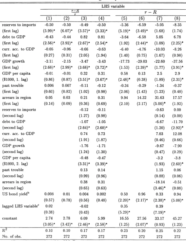
1000 USD), an indicator of total past repayment troubles (arrears, relieves and reschedulings since 1970), the percentage of countries in the region with arrears (a special form of regional effects, being surprisingly powerful in diagnostic regressions). These regressions simply try to explain (in fact: they capture quite a large part of) the interest surcharge (the risk premium) faced by a country. The results are contained in Table 1.1.

The overall fit of the R specification is around an R2 of 0.1, it goes up to 0.2 for the more linear r - R case. These are not extremely good fits, but we see that these variables do have reasonable explanatory power. One main reason for the low R2 is that many

observations correspond to multiple bond spreads in the same country-year cell, and none

of the within-cell variation can be captured by the explanatory variables. If one regressed

the average values on the same right hand side,l7 the point estimates would be very similar

and the fit would improve significantly (to .22 in the rR case and .52 in the r-R case). This

first fact also supports the initial hypothesis that the within-cell variations are orthogonal

to the right hand side variables.

We see that the lagged dependent variable is not significant in the rR specification, but

it is in the r - R case. This means that there is some effect of past private information on the

current spread, but not with the other functional form choice. It is even possible, however,

to have a variable (say v) insignificant in the reduced form and still cause a rejection of the overidentification test:: if the event at hand is such that v is highly correlated with it, then this variable has an indirect effect A72v y- 0 on the spread, so the residual will contain

(74 - Ay2)v 0 0, and it might be not offset by the other variables. And as we will see, this

lagged value will play an important role in forthcoming estimations.

The inclusion of further lags helps in both cases, but does not improve the fit meaning-fully. Nevertheless, it shakes the point estimates (and the standard errors) substantially: as most of the variables are highly correlated with past values, this symptom of multicollinear-ity is not surprising. It also legitimates the choice of not using both lags as instruments, but only the first one.

Apart from these, I do not want to read any strong stories from these descriptive results: first, some multicollinearity might be present even within the first lags of the variables; and

1774 observations and 10 explanatory variables: US bond rate, lagged dependent variable, constant and

Table 1.1: Describing bond yieldsa LHS variable

r-K

r-R

T reserves to imports (first lag) debt to GDP (first lag) curr. acc. to GDP (first lag) GDP growth (first lag) GDP per capita ($1000, 1. lag) past trouble (first lag) arrears in region (first lag) reserves to imports (second lag) debt to GDP (second lag) curr. acc. to GDP (second lag) GDP growth (second lag) GDP per capita ($1000, 2. lag) past trouble (second lag) arrears in region (second lag) US bond yieldb lagged LHS variablec constant R2 No. of obs.

a All equations are e

(1) (2) (3) -0.50 -0.50 -0.49 (5.99:* (6.07)* (3.57)* -0.43 -0.44 0.82 (2.56:* (2.92)* (2.67)* -O.O05 -0.06 -0.66 (0.27) (0.31) (2.05) -2.11]. -2.15 -3.47 (2.68:1* (2.99)* (3.68)* -0.01. -0.01 0.32 (0.86) (0.87) (3.51)* 0.006 0.007 -0.11 (0.60) (0.82) (1.02) 0.05 0.03 0.21 (0.14) (0.09) (0.36) -0.12 (1.27) -1.07 (2.64)* 0.74 (1.91) -1.76 (1.24) -0.48 (3.31)* 0.13 (0.99) 0.38 (0.65) 0.008 0.01 0.004 (0.57) (0.78) (0.56) 0.02 -0.02 (0.38) (0.43) 2.74 2.78 6.09 (3.05 * (3.42)* (2.46)* 0.10 0.10 0.17 272 272 272 stimated by OLS. T (4) -0.50 (3.33)* 0.81 (2.54)* -0.63 (1.94) -3.43 (3.72)* 0.31. (3.67)* -0.12 (0.98) 0.31 (0.69) -0.11 (0.98) -1.05 (2.60)* 0.73 (1.87) -1.71 (1.30) -0.47 (3.39)* 0.14 (0.96) 0.31 (0.63) 0.002 (0.48) 5.99 (2.58)* 0.17 272 (5) -5.36 (5.19)* -3.64 (1.92) -6.40 (1.40) -17.73 (1.53) 0.58 (2.48)* -0.34 (2.06) 9.94 (2.10) 0.50 (2.20)* 0.35 (5.29)* 16.55 (1.25) 0.23 272 (6) (7) -6.59 -5.05 (3.49)* (1.68) -6.58 5.05 (2.44)* (1.09) -4.76 -10.03 (0.75) (1.67) -29.03 -22.60 (2.39)* (1.77) 0.13 2.5 (0.38) (1.89) -0.29 -1.34 (1.43) (1.23) 14.32 31.63 (2.17) (5.00)* -0.63 (0.14) -6.67 (1.20) 7.03 (0.46) -9.67 (0.47) -3.2 (1.93) 1.15 (0.88) -18.14 (3.46)* 0.96 0.33 (2.17)* (2.38)* 0.39 (7.19)* 27.56 33.17 (2.07)* (0.93) 0.20 0.25 272 272 (8) -8.35 (1.74) 6.78 (2.25)* -8.26 (0.98) -37.56 (3.91)* 2.9 (2.31)* -0.37 (0.40) 17.57 (1.92) 0.00 (0.00) -11.70 (2.92)* 12.08 (0.66) -7.90 (0.29) -3.8 (2.60)* 0.06 (0.06) -0.51 (0.08) 0.94 (5.08)* 45.27 (1.23) 0.22 272

statistics are in parentheses. They are robust to clustering at the country level. * denotes significance at the 95% level..

b US bond yield is the yield on long-term (10 years) US government bonds.

c Lagged LHS variable is calculated as the average of all bonds of the same country one year ago; or two years

ago if no data for previous year.

-second, many further variables can be included on the right hand side (in a very extreme

rational expectations approach: all information available at the time of price formation),

causing a missing variable bias in the reduced form estimates.

I still point out some counter-intuitive signs among the estimates: for example, a higher

debt to GDP ratio seems to decrease spreads, and a higher GDP per capita tends to increase

spreads. Though it may be due to some data problems (sample, multicollinearity, missing

variables), but we will get some further interpretation from the prediction equations later

on.

As all the future results will be a refinement of these reduced forms, their overall fit can be at most as good as these fits.l8 The refinements are obtained in the following manner:

when replacing the right hand side with a +

/dit,

I force a

4

,

64, r4

and 64 to be such that

C4 +

4

Rt + r4'Zit + 6

4

Hit = a +

A

(a2 + P

2

Rt + r2Zit + 6

2

Hit) + 6Hit

holds. The overidentification will reject exactly when this interpretation of the reduced form is not acceptable. Such a rejection tells us that the premium is coming from a different source of risk: maybe only the choice of my event indicator is off from the right one, or maybe the "true" event is completely different.l9

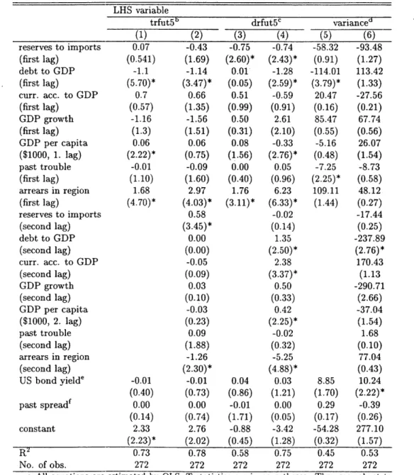
Before actually switching to the structural form, I need to discuss briefly the first stages of all structural form estimations: the linear probability equations (Table 1.2) - which are in fact measuring how correlated the instruments are with the right hand side events.

One feature of the results is the surprisingly high R2: 0.6-0.7 for the different default

indicators, and around 0.5, for price volatility. This means that the set of instruments I am

working with is highly correlated with the variables for which they are instrumenting.

There is a saddle issue here: in order to interpret the high R2 as high correlation of the instruments and the events, I kept the same multiple country-year cells (the number of observations stayed 272). However, this means that I am simply using some observations

more than once (the only variable in which they are different is the bond yield). To check

18I will not, in general, report any R2 values from the forthcoming two-stage estimations, as the R2does not correctly measure the fit of a two-stage procedure. Instead, I will use the value and the p-value of the

F test of joint significance.

'90ne can also say that maybe the spread has components completely unrelated to any particular risky

events - my goal is, however, to see how far I can get in identifying certain risks as being the main source

Table 1.2: The prediction equationsa

LHS variable

trfut5b drfut5c varianced

(1) (2) (3) (4) (5) (6) reserves to imports 0.07 -0.43 -0.75 -0.74 -58.32 -93.48 (first lag) (0.541) (1.69) (2.60)* (2.43)* (0.91) (1.27) debt to GDP -1.1 -1.14 0.01 -1.28 -114.01 113.42 (first lag) (5.70)* (3.47)* (0.05) (2.59)* (3.79)* (1.33) curr. acc. to GDP 0.7 0.66 0.51 -0.59 20.47 -27.56 (first lag) (0.57) (1.35) (0.99) (0.91) (0.16) (0.21) GDP growth -1.16 -1.56 0.50 2.61 85.47 67.74 (first lag) (1.3) (1.51) (0.31) (2.10) (0.55) (0.56) GDP per capita 0.06 0.06 0.08 -0.33 -5.16 26.07 ($1000, 1. lag) (2.22)* (0.75) (1.56) (2.76)* (0.48) (1.54) past trouble -0.01 -0.09 0.00 0.05 -7.25 -8.73 (first lag) (1.10) (1.60) (0.40) (0.96) (2.25)* (0.58) arrears in region 1.68 2.97 1.76 6.23 109.11 48.12 (first lag) (4.70)* (4.03)* (3.11)* (6.33)* (1.44) (0.27) reserves to imports 0.58 -0.02 -17.44 (second lag) (3.45)* (0.14) (0.25) debt to GDP 0.00 1.35 -237.89 (second lag) (0.00) (2.50)* (2.76)* curr. acc. to GDP -0.05 2.38 170.43 (second lag) (0.09) (3.37)* (1.13 GDP growth 0.03 0.50 -290.71 (second lag) (0.10) (0.33) (2.66) GDP per capita -0.03 0.42 -37.04 ($1000, 2. lag) (0.23) (2.25)* (1.54) past trouble 0.09 -0.02 1.68 (second lag) (1.88) (0.32) (0.10) arrears in region -1.26 -5.25 77.04 (second lag) (2.30)* (4.88)* (0.43) US bond yielde -0.01 -0.01 0.04 0.03 8.85 10.24 (0.40) (0.73) (0.86) (1.21) (1.70) (2.22)* past spreadf 0.00 0.00 -0.01 0.00 0.29 -0.39 (0.14) (0.74) (1.71) (0.05) (0.17) (0.26) constant 2.33 2.76 -0.88 -3.42 -54.28 277.10 (2.23)* (2.02) (0.45) (1.28) (0.32) (1.57) R2 0.73 0.78 0.58 0.75 0.45 0.53 No. of obs. 272 272 272 272 272 272

a All equations are estimated by OLS. T statistics are in parentheses. They are robust to clustering at the country level. * denotes significance at the 95% level. The results for "relpdf5" - the sum of the relief to debt stock ratios in the next five years (including the current one) - are not reported, but quite similar.

b The variable "trfut5" is an indicator of debt relief, rescheduling or arrears in the next 5 years (including the current one).

c "drfut5" is similar to "trfut5" but does not include arrears.

d Variance is 5-year the empirical variance of all bond spreads of the country starting from next year.

e The lagged spread is calculated as the average of all spreads one or two years ago.

how much difference it makes, I reran the same linear probability models with country-year averages. The results are quite similar, there are no large and significant changes in the estimates.2 0 The R2 changes to around 0.6 for the default indicators, and reduces to 0.4 in the variance case (using single lags for all three).

The second lags increase the R2 by 0.05-0.18, so they do improve the fit, but the fit is already acceptable with only the first lags. We see the multicollinearity of the lags again, which shows that using the second lags as additional instruments might even cause imprecise

2SLS estimates.2 1

Returning to the counter-intuitive signs from the reduced form, we can see that a higher

debt to GDP ratio decreases the predicted variance of the spread, and it has a negative

sign in general whenever it is significant (at least the first lag). Past repayment trouble does not influence risk predictions, but it lowers the variance significantly. So if these risk predictions have a positive effect on the spread (and this is the case, as we will see soon), then a higher debt to GDP ratio can in fact lower spreads, by making bond markets more liquid, prices less volatile and hence decreasing the illiquidity risk by more than increasing the default risk (if increasing at all).

The yield on US bonds is marginally significant for the variance term. The past value of r - R is insignificant in all cases (all conclusions remain true for the country-year average estimation). Since the lagged value was significant in the spread specifications of Table 1.1, these two findings together suggest that there is extra information incorporated to the

spreads, but it is not related directly to repayment troubles or liquidity shocks of the bonds.

Having checked our instruments in terms of being or not correlated with dit and lit, we

can turn to estimating (1.7) now. The question is whether we can attribute the fit of the

reduced form entirely to (2 +2Rt + /2Rt + r2Zit) or not. Since the R specification seems

much less appropriate, I will focus on r - R, and report some ---R results only as robustness

checks.

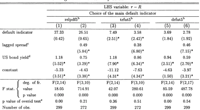
Table 1.3 reports the results for only with default risk included on the right hand side. In columns 1 and 2, the choice of the default indicator is the ratio of debt forgiven (in the

20

The only major change is that the sign of GDP per capita changes in the "trfut5" specification, it stays

small but significant.

21In general, using more good instruments reduces the standard errors, but due to small sample properties of 2SLS, it might also produce a higher bias. I chose these particular variables since they are reasonably correlated with the event indicators, and also as a tradeoff between a larger and an even smaller set. I will

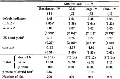
next 5 years) to current debt stock; in 3 and 4, debt relief, rescheduling or arrears in the next 5 years; finally, 5 and 6 uses only relieves and reschedulings. The coefficient on the default risk indicator is always at least marginally significant and large: a 1 percent relief increases the spread by 26-27 basis points; a 10 percent increase in all predicted repayment troubles adds 35-74 basis points, and 27-36 if it is only predicted relief or rescheduling.

Table 1.3: Regression results: only default risk considereda LHS variable: r - R

Choice of the main default indicator

relpdf5b trfut5b drfut5b

(1) (2) (3) (4) (5) (6) default indicator 27.33 26.51 7.49 3.58 3.69 2.78 (0.42) (0.65) (2-.51)* (2.42)* (1.84) (1.92) lagged spread' 0.49 0.38 0.46 (5.84)* (6.80)* (7.15)* US bond yieldd 1.18 0.75 1.18 0.86 0.94 0.59 (I5.52)* (3.29)* (7.90* (6.34)* (2.51)* (2.70)* constant -5.23 -4.43 -11.12 -7.63 -4.63 -3.97 (3.51)* (3.38)* (4.31* (4.34)* (1.50) (3.21)* deg. of fr. F(2,14) F(3,10) F(2,14) F(3,10) F(2,14) F(2,17) F stat. value :18.05 714.91 42.07 280.61 85.59 487.78 p value 0.000 0.000 0.000 0.000 0.000 0.000 p value of overid teste 0.00 0.21 0.36 0.51 0.00 0.54 Number of obs. 299 272 299 272 299 299

a All estimations are IV, using lagged values of reserves to imports, debt to GDP, current account balance to GDP, GDP growth, GDP per capita, past repayment troubles, arrears in region and US government bond yields as instruments. T statistics are in parentheses. They are robust to clustering at the country level. * denotes

significance at the 95% level.

b "relpdf5" is the sum of the relief to debt stock ratios in the next five years (including the current one). "trfut5" is an indicator of debt relief, rescheduling or arrears in the next 5 years (including the current one). "drfut5" is similar to "trfut5" but does not include arrears.

c The lagged spread is calculated as the average of all spreads one or two years ago. d US bond yield is the yield on long-term (10 years) US government bonds.

e The overidentification test regresses the residuals on the right hand side variables and instruments.

The fit always increases when the lagged spread is included, its coefficient is stable around 0.4-0.5, highly significant. This may indicate country-specific fixed effects, or, as I will argue later, some adjustments to the risk events (the difference between my choice and the "true" choice). For overidentification to pass, we almost always need to include the lagged value (with the exception of column 3). Column 3 indicates that the chance of any kind of financial trouble is very influential in determining the spreads: in other words, bond spreads do reflect the overall chance of repayment problems, but those problems, for some reasons, ended up not leading to bond defaults. Once including more than one event

at the same time, the more restrictive default indicator and the price volatility term will

yield a more substantive risk decomposition (into default and liquidity risk), so I will use

that as the main specification later on.

The last important feature of the results is the surprisingly stable (0.6-1.18) and

sig-nificant coefficient of the US interest rates. This implies that spreads increase nearly one in one with the US interest rate, above any potential effect through increased default risk. This can indicate important aggregate liquidity effects, or investors may be less eager to hold risky bonds when even safe bonds offer high returns. Once I include the price volatility term, most of the effect of US rates will go through that term; so US interest rates will have a much smaller effect above their influence over default and liquidity risk.

1.4.2 Identification and generalization of the method

There is a very important and general interpretation of the entire approach I am using.

Certain variables Zit and some others have explanatory power in an asset pricing (bond spread) equation:

ritj

-

Rt = a + Rt +

rZit +

Eitj

This is the standard approach in the literature (though usually with logistic probability

models or some other variations). However, to understand where these relationships are coming from, one needs a structural approach. Assume that the spread reflects some mea-sure of the risk of a certain event (this might be a zero-one, or a continuous variable). Use a rational expectations (linear) prediction of that event of the form

eit =

a'

+ 3'Rt + r'Zit + eit.

If the spread is coming from the risk of this event, then

ritj - Rt =

("

+

A"E[eitlRt,

Zit] + sit

j

should describe the spread. Using the best linear prediction of the conditional expectation (or, in a more robust sense, doing the IV process mentioned in the introduction and discussed

in more details later in the subsection), one gets

rit -Rt = cr" +

A"

(aI

+

8'Rt +

rZit)

+ E.. = a" + A"eit + itj

This means that one tries to attribute the fit and explanatory power of R and Z to their

predictive power for (correlation with) the event e. Then a rejection of the overidentification

means that either the choice of the event is not perfectly right (or at least, there is something

else also playing a role), or that expectations are not fully rational.

Unless one has a very strong case for a particular choice of a (default or any other) event,

it is impossible to distinguish the rejection of rational expectations from the rejection of the

choice of the event. I will maintain rational expectations, and at the same time, introduce

different choices of the event e - maybe even more than one event at a time.

For foreign-currency denominated sovereign bonds, the two major choices will be a repayment difficulty ("default") variable, and an illiquid markets indicator.2 2 Once I have

both of these probabilities incorporated into the interest rate equation, I can check whether

one or the other is enough to explain the country-time variation of bond spreads.

The treatment of the illiquidity event is the same as earlier: one specifies a linear

prediction model for actual future illiquidity shocks

lit =

₃

+

f

3

Rt + r

3

Zit + E3it,

(1.9)

and then add

E[litIRt,

Zit] = a3 + /3Rt + r3Zit to

(1.7A):

rit - Rt = a + fRt + A

1

(a2 +

2

Rt + r

2

zit) +

2

(a

3

+ 3

3

Rt + r

3

Zit) +

+ itj

(1.7B)

What is this event lit?' One proxy could be the following: whenever the current rR or

r - R is high, it means that the current price is much lower than what a safe and liquid

bond would have. If I assume that this movement does not entirely reflect a sudden increase

in the default risk of the bond, then it is a time when the market for these bonds "dries

out". So one can define an event indicator for r-R or r - R being above certain thresholds at least once in the next (say) 2 years.

2 2_{With local-currency denominated bonds, a devaluation risk event could and should be introduced in a}

I experimented with many choices of this indicator: different threshold levels and

differ-ent time windows. In general, it turns out not to be a very successful choice for disdiffer-entangling illiquidity from default risk: if low future prices are mostly reflecting higher perceived de-fault risk, then this illiquidity variable might not be distinguishable enough from dede-fault risk - and this is what the results show. So instead, the (sample) variance o