Fuzzy Bilevel Optimization
By the Faculty of Mathematik und Informatik
of the Technische Universität Bergakademie Freiberg
approved
Thesis
to attain the academic degree of doctor rerum naturalium
(Dr.-rer. nat.)
submitted by
Dipl.-math. Alina Ruziyeva
born on the 8. Mai 1986 in Almaty (Kazakhstan) Assessor: Prof. Dr. Stephan DempeProf. Dr. Andreas Fischer
Versicherung
Hiermit versichere ich, dass ich die vorliegende Arbeit ohne unzulässige Hilfe Dritter und ohne Benutzung anderer als der angegebenen Hilfsmittel angefertigt habe; die aus fremden Quellen direkt oder indirekt übernommenen Gedanken sind als solche kenntlich gemacht. Die Hilfe eines Promotionsberaters habe ich nicht in Anspruch genommen. Weitere Personen haben von mir keine geldwerten Leistungen für Arbeiten erhalten, die nicht als solche kenntlich gemacht worden sind. Die Arbeit wurde bisher weder im Inland noch im Ausland in gleicher oder ähnlicher Form einer anderen Prüfungsbehörde vorgelegt.
I hereby declare that I completed this work without any improper help from a third party and without using any aids other than those cited. All ideas derived directly or indirectly from other sources are identied as such.
I did not seek the help of a professional doctorate-consultant. Only those persons identied as having done so received any nancial payment from me for any work done for me. This thesis has not previously been published in the same or a similar form in Germany or abroad.
v
Acknowledgement
First of all I would like to express my deepest gratitude to my supervisor Prof. Dr. Stephan Dempe for giving me the opportunity to pursue my PhD studies at TU Bergakademie Freiberg and for his continuing support over the years.
All the colleagues and sta members of the Department of Mathematics and Computer Science of TU Bergakademie Freiberg deserve my special thanks for providing me with a pleasant working environment.
Last but not least, I would like to sincerely thank my ancé Michael and my mother Raisa for their support and trust.
vii
Contents
1 Introduction 1 1.1 Why optimization . . . 1 1.2 Fuzziness as a concept . . . 2 1.3 Bilevel problems . . . 6 2 Preliminaries 11 2.1 Fuzzy sets and fuzzy numbers . . . 112.2 Operations . . . 15
2.3 Fuzzy order . . . 16
2.4 Fuzzy functions . . . 17
3 Optimization problem with fuzzy objective 19 3.1 Formulation . . . 19
3.2 Solution method . . . 20
3.3 Local optimality . . . 24
3.4 Existence of an optimal solution . . . 25
4 Linear optimization with fuzzy objective 27 4.1 Main approach . . . 28
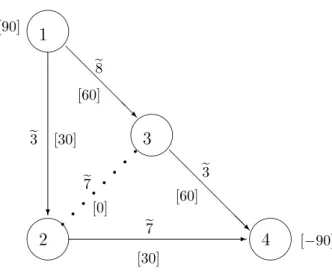
4.2 Example . . . 30
4.3 Optimality conditions . . . 33
4.4 Membership function value . . . 34
4.4.1 Special case of triangular fuzzy numbers . . . 36
4.4.2 Example . . . 39
5 Optimality conditions 47 5.1 Dierentiable fuzzy optimization problem . . . 48
5.1.1 Basic notions . . . 48
5.1.2 Necessary optimality conditions . . . 49
5.1.3 Sucient optimality conditions . . . 49
5.2 Nondierentiable fuzzy optimization problem . . . 51
5.2.1 Basic notions . . . 51
5.2.2 Necessary optimality conditions . . . 52
5.2.3 Sucient optimality conditions . . . 54
5.2.4 Example . . . 55
6 Fuzzy linear optimization problem over fuzzy polytope 59 6.1 Basic notions . . . 60
6.3 Formulation and solution method . . . 65
6.4 Example . . . 69
7 Bilevel optimization with fuzzy objectives 73 7.1 General formulation . . . 74
7.2 Solution approaches . . . 74
7.3 Yager index approach . . . 76
7.4 Algorithm I . . . 77
7.5 Membership function approach . . . 78
7.6 Algorithm II . . . 80
7.7 Example . . . 81
8 Linear fuzzy bilevel optimization (with fuzzy objectives and constraints) 87 8.1 Formulation . . . 87 8.2 Solution approach . . . 88 8.3 Algorithm . . . 90 8.4 Example . . . 91 9 Conclusions 95 Bibliography 97
1
1 Introduction
1.1 Why optimization
The mathematical area of optimization plays a very important role in our modern life. In our age of scarce natural resources such as oil and gas, it is particularly important not to waste. This requires an optimal use of these supplies. The same applies to other limited resources as well a time. This strive for optimal solutions is not limited to industrial applications but has long reached our daily life.
Our quest is complicated by the fact that we - more often than not - have to make decisions without being able to rely on precise information. We have to deal with an amount of uncertainty every single day. Moreover, our understanding of linguistic variables often depends on e.g. mood. Let us consider the phrase "The shop is near the house". In terms of fuzzy logic we understand word "near" dierently. It strongly depends on the age of the decision making person (or decision-maker for short). Thus, the young decision-maker can say that the phrase is true, even if the distance from the house to the shop exceeds 2 km. For the old person, the phrase holds true only if the distance is less than, say, 800 m. Of course, in this example we have to dene what words "young" and "old" mean. However, it becomes now clear that dierent persons dene usual things dierently. Thus, it makes perfect sense to speak about fuzzy optimization problems from a vague predicate approach, as it is understood that this vagueness arises from the way we express the decision-makers' (i.e. our) knowledge and not from any random event. In short, it is supposed that the nature of the data dening the problem is fuzzy.
In practical situations, the problem of optimization is even more complicated, since it involves conict resolution. Each partly involved decision-makers try to maximize their own benets. Such an optimization problem can be illustrated with the following example of gas use: The government tries to maximize prot with its tax-policy for private gas companies. In turn, those companies try to maximize their prot by setting a price for gas. Consumers decide on which company to choose by comparing prices. They try to minimize costs by choosing the company that oers a smallest gas price. The easiest way for the government is to prescribe innitely large taxes. But with such a policy it will loose all the companies and a region (e.g. a city) can be left without any gas. Therefore, the government has to establish taxes wisely. Each company, in turn, has to x prices which are acceptable for the clients. Otherwise, the clients choose another corporation. Multilevel optimization problems are important for decentralized organizations and sys-tems, where each unit (or department) seeks its own interest. Carefully dened multilevel mathematical programming problems can also serve as useful tools in modelling structured economic units.
In the present work we focus our attention on a special case of multilevel optimization, namely bilevel optimization. We discuss hierarchical problems of two decision makers,
in which one - the called leader - has the rst choice and the other one - the so-called follower - reacts optimally on the leader's selection. It is important to note, that each decision-maker maximizes his / her own benets independently, but is aected by actions of the other decision-maker (through externalities). The formulation of the bilevel programming problem for crisp (i.e. with exactly known and xed) data can be found e.g. in the book of Dempe (2002).
1.2 Fuzziness as a concept
In crisp optimization problems it is assumed that the decision-maker has exact and full information on the data entering the problem. Even when this is the case, the decision-maker usually nds it more convenient to express his / her knowledge in linguistic terms, i.e. through conventional linguistic variables (see e.g. Zadeh (1975a,b,c)), rather than by using high precision numerical data.
One commonly used approach to deal with these problems is to model them as fuzzy optimization problems, see e.g. Zadeh (1965). This approach proved to be very useful in many applied sciences, such as engineering, economics, applied mathematics, physics, as well as in other disciplines: Buckley and Feuring (2000); Chanas and Kuchta (1996a); Jiménez et al. (2006); Kasperski and Zieli«ski (2006); Peidro et al. (2010); Weber et al. (1990); Wu and Xu (2008); Wu et al. (1997); Zimmermann (1978); Zhang et al. (2010); Zimmermann (1976). Among linear programming problems, the so-called transportation problem is very popular, see e.g. Chanas and Kuchta (1996a); Shih and Lee (1999). The model which customarily has been referred to as transportation problem represents not only delivery planning problem with given supplies and demands and with a criterion of minimizing the total transportation cost. Many other decision-making problems, whose motivation is quite dierent from that of the delivery planning, have the same mathe-matical structure. For example, this is the case for the periodical production planning problem with given demands for the product in consecutive periods and with the criterion of minimizing the total production and storage cost.
There exist eective algorithms solving the transportation problem in the case when all coecients in the model, i.e. supply and demand values as well as the unit transportation costs, are given in a crisp way. In practice, however, this condition may not be fullled. For example, the unit transportation costs are rarely constant and predictable. Therefore, the ability to dene and to determine the optimal solution of the transportation problem with fuzzy costs coecients is important. This is exactly the topic of most examples presented in the present work.
In the thesis the following (nonlinear) fuzzy optimization problem is investigated, where the objective function has fuzzy values and the constraint function is a crisp one, i.e.:
e
f(x)→min
g(x)≤0. (1.1)
Here g = (g1, . . . , gk) : Rn → Rk is a crisp function and fe:Rn → F is a fuzzy function,
whereF is a set of fuzzy numbers over R and 1≤ k <∞, 1≤n <∞. The investigated problem can be transformed into a more general problem where the constraint function
1.2 Fuzziness as a concept 3
is fuzzy. The formulation of fuzzy optimization problems with crisp objective and fuzzy constraints can be found in Delgado et al. (1989) and Tanaka et al. (1984).
An early approach for solving a fuzzy optimization problem is the extension principle of Bellman and Zadeh (1970). Even nowadays many authors base their solution algorithms on this approach (see e.g. Ekel et al. (1998)). In the present work fuzzy optimization problem (1.1) is solved with modern solution algorithms based on the minimization of a certain α-cut on the feasible set (see e.g. Chanas and Kuchta (1994, 1996b); Dempe and Ruziyeva (2011); Rommelfanger et al. (1989); Zimmermann (1991)).
In this approach fuzzy optimization problem (1.1) is reformulated into an interval op-timization problem
[fL(x, α), fR(x, α)]→min
g(x)≤0 (1.2)
for a certain level-cut α (0 ≤ α ≤ 1) of the fuzzy function f(x)e . Through the agency
of a special order for the intervals dened later, both of the left- and right-side functions fL(x, α)and fR(x, α)have to be minimized simultaneously.
Thus, a crisp biobjective optimization problem arises fL(x, α)→min
fR(x, α)→min
g(x)≤0,
(1.3)
that is solved, in turn, with application of methods of the multiobjective optimization problem's scalarization technique (see e.g.Ehrgott (2005)). Elements of the Pareto set of each biobjective optimization problem are interpreted as solutions of the initial fuzzy optimization problem on a certain level-cut. Thus, we reect incomparability (and vari-ability) of the solutions of the fuzzy optimization problem. This discussion is presented for the general case in Chapter 3.
The problems usually considered in optimization are mathematical models and, thus, idealizations of real world problems. Therefore, the classical "achieve the best value of the objective function" approach may be too restrictive. Often a set of alternative solutions is more valuable to the decision-maker.
Many authors (see e.g. Jiménez et al. (2006); Verdegay (1982)) try to nd a single best solution of the fuzzy optimization problem in the linear case
e
c>x→min Ax≤b
x≥0,
(1.4)
where the fuzzy vectorec, the constraint matrix A∈R
m×n and the right-hand side vector
b ∈ Rm are given. These approaches are based on the extension principle of Bellman and Zadeh (1970). We suggest to reect the uncertainty in fuzzy optimization problems through (the existence of) a set of optimal solutions, i.e. a set of Pareto optimal solutions of corresponding biobjective optimization problem. Under the assumption that this set consists of more than one element, the decision-maker can improve the choice relying on some criteria that are not a priory considered in the optimization problem.
Therefore, it is natural to consider the solutions of a fuzzy optimization problem as fuzzy. Hence, a criterion for comparing the elements of the fuzzy set of optimal solutions is required. As soon as this fuzzy set has membership function, the possible criteria for comparison the elements of the fuzzy solution can be the values of the membership function. For this it is necessary to compute the values of the membership function exactly. An approach to calculate such membership function values is suggested by Chanas and Kuchta (1994, 1996a,b) and further developed by Dempe and Ruziyeva (2012).
The approach to determine the membership function values is based on calculating the sum of lengths of certain intervals. One of the purposes of the present work is to realize this idea based on modern solution algorithms (see e.g. Cadenas and Verdegay (2009); Chanas (1983); Chanas and Kuchta (1994, 1996b); Jiménez et al. (2006); Rommelfanger et al. (1989); Zimmermann (1978)). Our solution approach for fuzzy linear optimization problem (1.4) is based on the reformulation of the well-known optimality conditions for the crisp linear optimization problem (see e.g. Bertsimas and Tsitsiklis (1997)).
With this innovative approach, published in Dempe and Ruziyeva (2012), the decision-maker obtains a collection of some basic solutions, each accompanied by a measure of the extent to which it is the optimal solution of fuzzy optimization problem (1.4). It is up to the decision-maker to make the nal choice - the decision-maker can restrict himself / herself to the solutions which are equal to a degree greater than a xed value, or the solutions which have membership function values greater than a xed value, or equal to one, etc. In any case our fuzzy solution will constitute an important support and source of information for the decision-maker.
In Chapter 4 we discuss the fuzzy linear optimization problem and derive explicit formu-las for the calculation the membership function value of the elements of the fuzzy solution in the case of triangular fuzzy numbers and show that only one certain interval needs to be considered.
Generalizing our approach to nonlinear fuzzy optimization problem (1.1), the question of optimality of a feasible solution arises, which is very important and essential in opti-mization. In the nonlinear case of the fuzzy optimization problem, using basic methods of convex multiobjective optimization, necessary and sucient conditions for an optimal solution of the dierentiable fuzzy optimization problem are derived e.g. in a form of Karush-Kuhn-Tucker optimality conditions.
Wu (2004) gave sucient optimality conditions for a solution of fuzzy optimization problem (1.1) under convexity assumptions. In Wu (2008) integrals in the Karush-Kuhn-Tucker conditions were used for sucient optimality conditions of fuzzy optimization problem (1.1). This means, the author used a certain average value of the level sets of the fuzzy objective function. In distinction, in Wu (2004) only one α-cut was used. Left-and right-hLeft-and side functions were used by Wu (2004, 2008) to describe the level-cuts of the fuzzy objective function which then appear in the Karush-Kuhn-Tucker optimality conditions.
For the dierentiable case of fuzzy optimization problem (1.1) we present sucient optimality conditions by using the Karush-Kuhn-Tucker conditions. It turns out that these conditions are similar to the sucient optimality conditions used in the works of Wu (2004, 2008). The distinction is the use of weighting coecients in the objective. Further, we derive necessary optimality conditions.
1.2 Fuzziness as a concept 5
In the dierentiable fuzzy case necessary and sucient optimality conditions are given by Dempe and Ruziyeva (2011) and in the nondierentiable crisp case by Bomze et al. (2010). If the fuzzy objective function f(x)e is nondierentiable, it requires some
modi-cations in the standard approach.
Adapting the notions of the tangent cone, the directional derivative and Hadamard derivatives to the fuzzy case permits us to derive necessary and sucient optimality con-ditions for a (global / local) optimal solution of the nondierentiable fuzzy optimization problem.
As soon as we dene a set of optimal solutions of fuzzy optimization problem (1.1) on some xed α-cut through the set of Pareto optimal solutions of biobjective optimization problem (1.3), we can derive necessary and sucient optimality conditions (for both dif-ferentiable and nondierentiable fuzzy optimization problems) to guarantee that a feasible point belongs to the fuzzy solution set. This result generalizes one obtained in Panigrahi et al. (2008); Wu (2007) in four important aspects:
1. The derivative of the fuzzy functionfe(x)is dened as a pair of functions which need
not to be an interval as it was supposed in the paper of Panigrahi et al. (2008). This assumption is unnecessary restrictive.
2. Not only sucient but also necessary optimality conditions are derived.
3. An optimality condition which is valid for all level-cuts at the same time is derived. 4. Nondierentiable (and nonconvex) problems are discussed.
Optimality conditions of the nonlinear fuzzy optimization problem are examined in Chapter 5 in detail.
The next interesting question is the generalization of the fuzzy optimization problem to a fuzzy optimization problem with fuzzy constraints. An evolutionary algorithm based on multi-objective approach was presented by Jiménez et al. (2006). A so-called interactive approach is developed by Ammar (2000). A shortcoming of this approach is predetermined level-cut.
A fuzzy optimization problem with fuzzy constraints have been examined for the linear case e.g. by Chanas (1983); Ekel et al. (1998); Werners (1987) using the min-max approach and Buckley (1995) using the possibilistic approach.
We present a solution algorithm for the linear case of fuzzy optimization problem dened as
F(ec, x) = d>ec→min s.t. ec∈P,
(1.5) whereP is a fuzzy polytope, d is a known crisp vector andecis a fuzzy variable.
Because of the vagueness, the decision-maker prefers to have not just one solution but a set of them, so that the most suitable solution can be applied according to his / her judgement.
Fuzzy optimization problem (1.5) is solved by taking level-cuts of the fuzzy polytope P
for all α∈[0,1]. Each α-cut, in turn, provides two crisp optimization problems F(cL(α)) = d>cL(α)→min
and
F(cR(α)) =d>cR(α)→min
s.t. cR(α)∈PR(α), (1.7)
where[cL(α), cR(α)] denotes theα-cut of fuzzy variableec. Let us denote the solution sets
of problems (1.6) and (1.7) are c∗L(α) and c∗R(α), respectively. Then, an optimal solution of the fuzzy optimization problem on the xedα-cut is a convex hull ofc∗L(α)and c∗R(α). The fuzzy solution of initial problem (1.5) is the union of these convex hulls for all level-cuts, i.e.
e
c∗ = [
α∈[0,1]
(conv{c∗L(α), c∗(1)} ∪conv{c∗R(α), c∗(1)}), (1.8) wherec∗(1) is an optimal solution of problem
F(c1) =d>c1 →min
s.t. c1 ∈P(1) (1.9)
for α = 1 under assumption that we operate with triangular fuzzy numbers. Ideas are investigated in Chapter 6.
1.3 Bilevel problems
Bilevel programming problems are challenging problems of mathematical optimization, which are interesting from the theoretical point-of-view (as special case in nonsmooth optimization) and have a variety of applications. Problems with a predominantly hierar-chical structure are often found in government policy, economic systems, nance and are especially suitable for conict resolutions.
Since its rst formulation by Heinrich von Stackelberg (1934) in market economy (in the context of unbalanced economic markets), bilevel optimization has successfully been applied to many real world problems: Bard et al. (1998); Bjørndal and Jørnsten (2005); Camacho (2006); Candler et al. (1981); Cassidy et al. (1971); Dempe (2002); Fortuny-Amat and McCarl (1981); Hobbs and Nelson (1992); Marcotte and Savard (2001); Parraga (1981). For the past twenty years transportation problems have been beneting from the formulation of advances in bilevel programming: Ben-Ayed (1988); Ben-Ayed et al. (1992); Dempe et al. (2009); Kim and Suh (1988); Labbè et al. (1998); Migdalas (1995), which cover issues like network design, revenue management and other trac control problems (where the transportation problem is on the lower level, depending on the parameter selected from the upper level).
Considering the inherently dicult nature of bilevel problems due to their nonconvexity, nonsmoothness and implicitly determined feasible set, it is dicult to design convergent algorithms, and the few algorithms that converge appear to be very slow most of the time. Even in the simplest case, i.e. when the upper and lower level problems are crisp and linear, the bilevel programming problem has been shown to be N P-hard (see Ben-Ayed
and Blair (1990); Blair (1992)).
One approach to solving bilevel optimization problems in the crisp case is based on its transformation into a one-level optimization problem using e.g. Karush-Kuhn-Tucker
1.3 Bilevel problems 7
optimality conditions. S. Dempe and co-workers investigated this problem as well as its optimality conditions, see e.g. Bialas et al. (1980); Dempe (1987, 2000, 2002); Dempe et al. (2006). However, this approach can not been shown to give a global optimal solution.
To solve crisp multilevel linear programming problems (bilevel programming problems are a special case) Shih et al. (1996) presented the so-called fuzzy approach. The authors allege that the solution of a multilevel linear optimization problem over a polytope is not necessarily situated at a vertex. This approach is based on predetermined tolerance limits as well as Bellman and Zadeh (1970) max-min approach. But this method has the vice that for some articially introduced membership function the hierarchical order can become redundant, i.e. the inclusion of other levels into the system will not aect the solution. Later Sinha (2003) showed that another technique based on fuzzy mathematical programming gives better solutions than that proposed by Shih et al. (1996). In this algorithm the author uses a payo matrix consisting in ideal solutions and the same tolerance limits as in Shih et al. (1996). However, the question of the existence of a feasible solution that is located in such a strongly restricted interval is not addressed.
Recently, numerous algorithmic approaches have been proposed for the special case of the linear bilevel optimization problem (also known as two-level linear sourse control prob-lem) by Bard and Moore (1990); Bialas and Karwan (1984); Dempe (1987). Using duality theory Shi et al. (2007) applied the k-th best algorithm to linear bilevel optimization problem in the case of multiple followers.
Several works tried to establish a relationship between multilevel and multicriterion programming problems (see e.g. Bard (1983); Wen and Hsu (1989)). Bialas and Karwan (1978); Marcotte and Savard (1991) have shown that Pareto and bilevel optimality are distinct concepts. Further evidence can be found in e.g. Candler (1988); Haurie et al. (1990). It should be noted that bilevel and bicriterial problems are often confused in literature (see e.g. Arora and Gupta (2009)).
All the aforesaid can be combined to the more complicated problem of fuzzy bilevel op-timization (also called fuzzy bilevel decision making in the literature), if the data involved in the bilevel optimization problem are only approximately known. While very important for number of applications, this problem is poorly investigated. A number of fuzzy bilevel programming problems can be found in Dempe et al. (2009); Dempe and Starostina (2006) and references therein. While some convergent algorithms for crisp bilevel problems al-ready exist in the literature (see e.g. Bard (1982); Bard and Moore (1990); Dempe (1987); Ishizuka and Aiyoshi (1992); Önal (1993); Tuy and Ghannadan (1998); Wen and Huang (1996); White and Anandalingam (1993); Wu et al. (1998)), solution strategies for fuzzy bilevel programming problems are an emerging new eld with a wide range of practical applicability.
In the case of crisp bilevel optimization problems many authors consider that the opti-mal solution is over polytope (see e.g. Calvete et al. (2011)), analogously we assume that we have fuzzy bilevel optimization problem over fuzzy polytope. Thus, we suppose that the optimal solution (and later we would be interested in best optimal solution) is located in one of the extreme points of the corresponding polytope. Strict denitions are given further in the work. At the moment the fuzzy bilevel optimization problem with fuzzy objective function is formulated as follows.
respect to x over a crisp polytope X. The leader, in turn, minimizes his / her objective function F(ec, x) over the given fuzzy polytope Ce. We assume that the fuzzy function
F(ec, x) is also bilinear. More formally, the fuzzy bilevel optimization problem can be formulated as F(ec, x)→min e c∈Ce s.t. x∈arg min x {f(ec, x) :x∈X}. (1.10) Let us denote the set of optimal solutions of lower-level optimization problem through Ψ(ec); that is to say
Ψ(ec) = arg min
x {f(ec, x) :x∈X}. (1.11)
In general, the problem of determining the best solution ec
∗ for the leader can be de-scribed as that of nding a vector of parameters for the fuzzy parametric optimization problem, which together with the response of the follower x(ec)∈ Ψ(ec)proves to give the best possible function value for the upper level objective functionF(ec, x). That is
” min e
c∈Ce
”{F(ec, x) :x∈Ψ(ec)}. (1.12) Strictly speaking, this denition of the fuzzy bilevel programming problem is valid only in the case of a uniquely determined lower level solution for each possibleec. The quotation
marks in (1.12) have been used to express this uncertainty in case of non-uniquely set of optimal solutions on the lower level. From now onwards those marks would be dropped.
As soon as we apply the approach presented in Chapter 4 to the lower level problem f(ec, x)→min
x∈X, (1.13)
more than one optimal solution can be obtained, i.e. in this case there can be multiple optima. That means, thatΨ(ec)not necessarily is a singleton for some permissibleec. If the upper level objective function is sensitive to dierent values of x ∈ Ψ(ec), it is necessary to give a rule of selection of an optimal x∗ ∈Ψ(ec) in order to evaluateF(ec, x).
Notice that there is no reason why both decision-makers should collaborate, i.e. it is not certain that the upper level decision-maker can enforce a particular choice of the lower level decision-maker.
There exist only few possibilities to deal with this problem of non-uniqueness. Namely, 1. Assume that the follower always selects the optimal decisions which give the worst values of F(ec, x). This is the pessimistic or strong approach (Lohse (2011)), which is used when the leader is not able to inuence the follower and is forced to choose an approach bounding the damage resulting from an unfavourable selection by the follower. The resulting problem is:
min ec∈Ce
φp(ec),
where φp(ec) = max
x∈Ψ(ec)F(ec, x).
2. Assume that the leader is able to inuence the follower, so that the last one always selects the variables x to provide the best value of F(ec, x). This results in the
1.3 Bilevel problems 9
so-called optimistic or weak approach (Dempe and Starostina (2007)), where the resulting problem is stated as
min e c∈Ce φo(ec), whereφo(ec) = min x∈Ψ(ec)F(ec, x).
3. In the case when none of the assumptions described earlier can be conceded, selection function approach (Dempe and Starostina (2006)) can be applied to the initial fuzzy bilevel optimization problem.
The selection approach 3. is quite new and it seems to be more appropriate for our needs. The aim of this approach is to compute a selection function x(ec)∈Ψ(ec).
In the present work two dierent algorithms for the solution of fuzzy bilevel optimization problem (1.10) are presented in Chapter 7. Those algorithms are based on the selection function approach and a switch between upper- and lower-level problems.
One possibility to compute a selection function x(ec) ∈ Ψ(ec) is to use Yager ranking indices to avoid the incomparability of the fuzzy vectors. As shown by Liu and Kao (2004), the Yager ranking indices approach can be very useful in solving (single level) fuzzy optimization problems. Then, the fuzzy bilevel optimization problem can easily be reformulated into a crisp bilevel optimization problem (see Yager (1981)). According to Liu and Kao (2004), an optimal solution for xed parameter is then taken as an optimal solution of the initial follower's fuzzy optimization problem. This approach can easily be extended to nonlinear convex fuzzy optimization problems.
Another approach is based on the calculation of membership functions values of the elements of the fuzzy solution on the lower level. The preferable optimal solution is supposed to have a maximal membership function value, i.e. according to Chanas and Kuchta (1994), the solution has the highest potential being realized by the follower. An algorithm for computation of a value of the membership function of the elements of the fuzzy solution is presented in Dempe and Ruziyeva (2012).
Using of stability regions and a switch between two problems it is possible to nd an optimal vector of coecients at the upper level of the fuzzy bilevel optimization problem such that the chosen solution on the lower level stays optimal in the fuzzy bilevel pro-gramming problem. By examining all possible regions of stability, we obtain the global optimal solution.
The fuzzy bilevel optimization problem with fuzzy objectives and fuzzy constraints leads to further increase in complexity. The aim is to investigate this problem for the linear case. The optimization problem is formulated as follows.
On the lower level the follower attempts to solve a fuzzy optimization problem f(ec, x) = p>1ec+p>2x→min
x (1.14)
subject to (ec, x)∈P:=P×P for the xed fuzzy vectorec. Here Pis a fuzzy polytope in
the space of fuzzy vectors Fn and P is a polytope in the space of real vectors Rm. Crisp coecientsp1 andp2 are supposed to be known. Here the set of optimal solutions of fuzzy optimization problem (1.14) is
Ψ(ec) = arg min
In turn, the leader minimizes his / her own linear objective function F(ec, x) = d>1ec+d>2x→min
e
c (1.16)
subject to(ec, x)∈P with known coecientsd1andd2. Then, a fuzzy bilevel optimizaiton problem is formulated as F(ec, x) = d>1ec+d>2x→min e c s.t. (ec, x)∈P x∈Ψ(ec). (1.17) For the linear case of the fuzzy bilevel optimization problems solution procedures have been proposed by Zhang et al. (2006) and Zhang and Lu (2010). The authors assumed that we are dealing with the fuzzy variables and fuzzy constants that have trapezoidal membership functions. The authors reformulate fuzzy bilevel optimization into a crisp optimization problem for the xed level-cut using the proposition that the weights of all the left- and right-hand side functions are given. This conicts with idea of bicriteria optimization. The same is done with the constraints on the both levels. After all branch and bound andk-th best algorithms are applied to the crisp bilevel optimization problem. Dempe and Starostina (2007) considered the fuzzy bilevel optimization problem with linear constraints. The authors followed Zimmermann (1978) and reformulated the fuzzy bilevel optimization problem into a crisp bilevel optimization problem, where the opti-mization task of both decision-makers is replaced by maximizing the minimum value of all the membership functions in the respective problems, i.e. the max-min approach was used.
Zhang et al. (2008) reformulated the fuzzy linear bilevel optimization problem into a linear bilevel biobjective optimization problem and then applied the Karush-Kuhn-Tucker approach to this crisp bilevel optimization problem.
In the thesis the selection function approach is applied to solve linear fuzzy bilevel opti-mization problem (1.17). The adoptedk-th best algorithm is based on takingα-cuts of the fuzzy polytope P and applying methods described in Chapter 6. It is proved that with
the solution algorithm the global optimal solution is obtained. Moreover, membership function values are calculated. Thus, it is possible to provide the leader with quantita-tive information concerning the superiority of one optimal solution over others. These derivations can be found in Chapter 8.
11
2 Preliminaries
In this Chapter we give denitions of fundamental concepts such as fuzzy set and its level-cut, fuzzy number and its level-level-cut, the space of fuzzy numbers and fuzzy vectors. This is presented in Section 2.1. Further we dene operations with fuzzy (and crisp) numbers in Section 2.2. We introduce a fuzzy order in Section 2.3, respectively. Denition of a fuzzy function is given in Section 2.4. These are the prerequisites required to discuss fuzzy (bilevel) optimization problems.
2.1 Fuzzy sets and fuzzy numbers
Let us begin with a general denition of a fuzzy set. Fuzzy sets are sets whose elements have degrees of membership. The concept was introduced by Lot A. Zadeh (1965) as an extension of the classical notion of a set. In classical set theory, the membership of elements in a set is assessed in binary terms according to a bivalent condition an element either belongs or does not belong to the set. By contrast, fuzzy set theory permits the gradual assessment of the membership of elements in a set. This is described with the aid of a membership function valued in the real unit interval [0,1]. Fuzzy sets generalize classical sets, since the indicator functions of classical sets are special cases of the membership functions of fuzzy sets, which only take values0or1. In fuzzy set theory classical bivalent sets are usually called crisp sets.
Denition 2.1. A fuzzy setCeis dened as a pair(C, µCe), whereC is a crisp set (C ⊂Rn)
andµCe :C →[0,1]is the membership function of the fuzzy setCe. For each elementx∈C,
the value of µCe(x) is called the grade of membership of x in Ce.
Corollary 2.1. The empty fuzzy setDe is dened with its membership functionµDe(x)≡0
for all x∈D, i.e. is the same as a crisp empty set.
Denition 2.2. The α-level set Ceα of the fuzzy set Ce is dened for a xed α ∈[0,1] as
the crisp set for which the degree of membership function exceeds or is equal to the level α:
e
Cα ={x|µCe(x)≥α}.
Corollary 2.2. It is obvious that forα, α0 ∈[0,1]such thatα≤α0, an inclusionCeα ⊇Ceα0
holds true.
Denition 2.3. A fuzzy set Ce is convex if and only if (i) for all x, y ∈ C and for all
λ∈[0,1] the following inequality holds true:
µ˜n ( x x 0 c 1 a b d
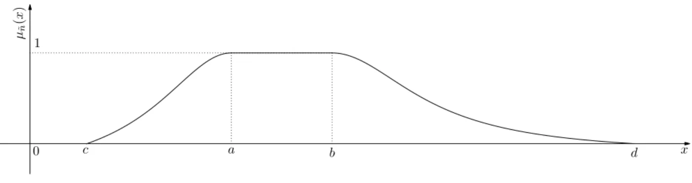
Fig. 2.1: A membership function of fuzzy numberne.
A fuzzy number is an extension of a regular number in the sense that it does not represent one single value but rather a connected set of possible values, where each possible value has its own "weight" between 0 and 1. This "weight" is called the membership function. A fuzzy number is thus a special case of a convex fuzzy set. A fuzzy numberecis
an element of the nonempty fuzzy setCeenriched with the nontrivial membership function
µec. In other words, a real fuzzy number is a convex continuous fuzzy subset of a real line.
More precisely, a fuzzy number was dened by Dubois and Prade (1978) as follows: Denition 2.4. A real fuzzy number en is a convex continuous fuzzy subset of the real
line, whose membership function µ˜n is
• a continuous mapping from R to the closed interval [0,1];
• constant on (−∞, c] :µn˜(x) = 0∀x∈(−∞, c];
• strictly increasing on [c, a];
• constant on [a, b]: µ˜n(x) = 1∀x∈[a, b];
• strictly decreasing on [b, d];
• constant on [d,+∞): µn˜(x) = 0∀x∈[d,+∞).
Herea, b, c and d are real numbers.
Within this Denition we say that µn˜(x) is the so-called truth value of the assertion
"the value of en is x". The membership function µn˜(x)can be seen in Fig. 2.1.
Remark 2.1. In general we can havec=−∞, ora=b, or c=a, or b=d, ord = +∞. Remark 2.2. If a = c = b = d, it is a crisp real number. If a = c and b = d, it is a representation of the tolerance interval [a, b] of the measurement of a quantity. If a =b, it is a representation of a fuzzy number, the value of which is "approximatelya".
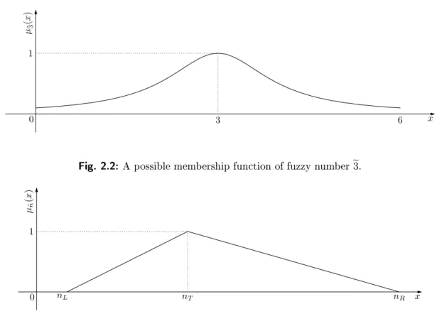
Example 2.1. A linguistic variable can be described as a fuzzy number. For instance, we say "about 3". That means, that the number is not well-dened. Thus, it can be represented as a fuzzy numbere3 with a membership function equal to
µ˜3(x) =
1
(x−3)2+ 1. (2.1)
2.1 Fuzzy sets and fuzzy numbers 13 µ˜ 3 ( x ) x 0 1 3 6
Fig. 2.2: A possible membership function of fuzzy numbere3.
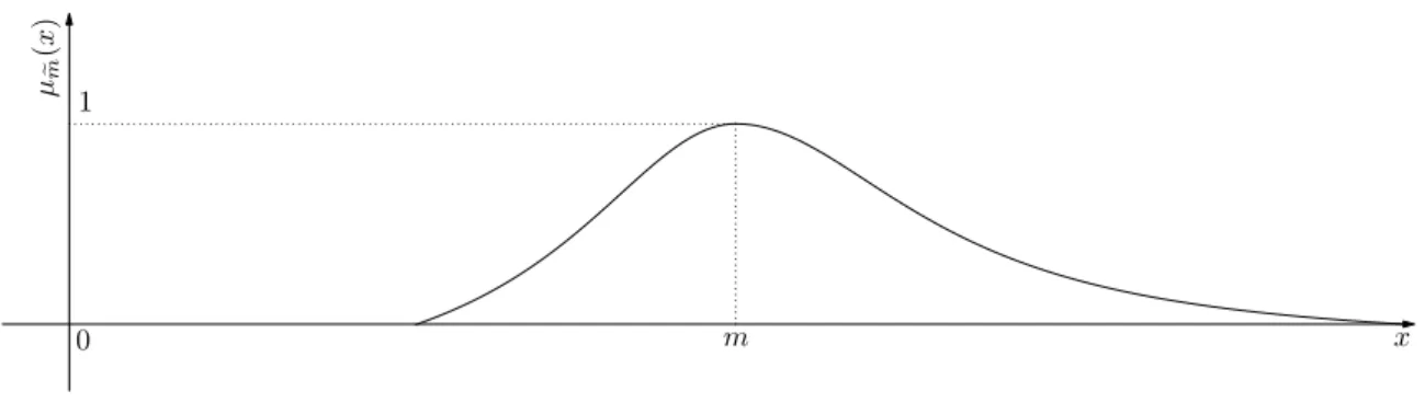
µ˜n ( x ) x 0 nL 1 nT nR
Fig. 2.3: A membership function of triangular fuzzy number en.
The simplest way to dene a fuzzy number en is presented by e.g. Buckley (1995) as
follows.
Denition 2.5. A continuous triangular fuzzy number ne is represented with a triple
(nL, nT, nR), where nL< nT < nR and the membership function µen is piecewise-linear.
A possible membership function of triangular fuzzy number en can be seen in Fig. 2.3.
Example 2.2. The fuzzy number e2 can be represented as a triple (0,2,6), i.e. its
mem-bership function is equal to
µ˜2(x) = ( 1 2x, x∈[0,2]; −1 4x+ 3 2, x∈[2,6]. (2.2) In the majority of examples presented in the present work we use triangular fuzzy numbers. The main reason is the straight forward interpretation of the triple(nL, nT, nR):
nT is the best estimate, nL is the minimum possible and nR is the maximum possible
values. There exist a generalization to Denition 2.5. It was shown by Dubois and Prade (1978), that a convenient representation for a fuzzy numberme is another triple (m, β, γ)
of parameters of its membership functionµme.
µem ( x x 0 1 m
Fig. 2.4: A membership function of the fuzzy LR-number me.
function µ(x) = L m−x β , if x≤m; Rx−γm, if x≥m. Here L and R are symmetric bell-shaped functions such that
L(0) =R(0) = 1.
m is called the mean value; β and γ are respectively named left and right spreads.
The example for a membership function of the fuzzy LR-number me can be seen in
Fig. 2.4.
Denition 2.7. A normalized fuzzy numberec is a fuzzy number with a membership
func-tion, that reaches value equal to 1:
maxµec(x) = 1 ∀x∈R.
In the present work it is assumed that all fuzzy numbers are normalized.
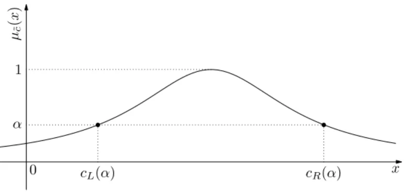
Denition 2.8 (Sakawa and Yano (1989)). The α-cut of a fuzzy number ea is dened as the ordinary set eaα for which its degree of membership function exceeds the level α
(α∈[0,1]):
e
aα ={a|µa˜(a)≥α}. (2.3)
An alternative denition is the following.
Denition 2.9. A level-cut (also called α-cut, α-level) of a fuzzy number ec is a special threshold described as an interval[cL(α), cR(α)]⊂Rfor some xedα ∈[0,1](see Fig. 2.5). HerecL(α) and cR(α) represent left- and right-hand side bounds of the fuzzy number econ
this certain α-cut.
Assumption 2.1. Without loss of generality, from now on we assume thate0 = 0, i.e.
µ˜0(x) =
(
1, x= 0; 0, x6= 0.
2.2 Operations 15 µ˜c ( x ) x 0 1 α cR(α) cL(α)
Fig. 2.5:α-cut of fuzzy numberec.
Let us extend the concept of a fuzzy set to a space of fuzzy numbers and a fuzzy number to a fuzzy vector.
Denition 2.10. A space of fuzzy vectors Fn is dened as a pair (Rn, µFn), where µFn :
Rn→[0,1] is a membership function of the elements of the fuzzy space Fn.
Remark 2.3. In the thesis we denote a space of fuzzy numbers through F, where µF :
R→[0,1].
Denition 2.11. A fuzzy vector ec is an element of the fuzzy space F
n enriched with a
nontrivial membership function µec.
2.2 Operations
Now we give some propositions concerning operations on fuzzy vectors. Operations on fuzzy numbers obviously are corollaries.
Proposition 2.1. Two fuzzy vectors are equal i they have the same membership func-tions, i.e. for ea, eb∈F
n
e
a=eb i µ˜a(x) = µ˜b(x) ∀x∈Rn.
Corollary 2.3. A fuzzy vector ea ∈ F
n is equal to a crisp vector a ∈
Rn i ea has the
following membership function:
µ˜a(x) =
(
1, x=a; 0, x6=a. Denition 2.12. Let ea,eb ∈ F
n. Then the sum of two fuzzy vectors
ea+eb is dened as a
fuzzy vector de∈Fn with the following property
dL(α) = aL(α) +bL(α) and dR(α) =aR(α) +bR(α) for all α ∈[0,1].
Here aL(α) and aR(α) are left- and right-side values of the fuzzy vector ea on a certain
Let A and B be two compact and convex subsets of Rn. If there exists a compact and convex subset C of Rn, such that A = B +C = {b+c : b ∈ B and c ∈ C}, then C is called the Hakuhara dierence of A and B. According to Banks and Jacobs (1970) we also writeC =AH B. Inspired by this concept, Wu (2008, 2009) dened the Hakuhara
dierence between two fuzzy vectors as following.
Denition 2.13. Let ea and eb be two fuzzy vectors in F
n. If there exists a fuzzy vector
ec ∈ F
n, such that
e
c+eb = ea (note that fuzzy addition is commutative) and ec is unique,
thenec is called the Hakuhara dierence of ea andeb and is denoted byeaHeb.
The following proposition follows from Denition 2.12 immediately, and is very useful for the future considerations of the dierentiation of fuzzy-valued functions.
Proposition 2.2. Letea,eb∈F
n. If the Hakuhara dierence
ec=eaHeb ∈F
n exists, then
cL(α) =aL(α)−bL(α) and cR(α) =aR(α)−bR(α) for all α∈[0,1].
Here[cL(α), cR(α)] is an α-cut of the fuzzy number ec.
A sum and a dierence of a fuzzy vector and a crisp vector are corollaries of Deni-tion 2.12 and ProposiDeni-tion 2.2.
Corollary 2.4. Let ea ∈ F
n and b ∈
Rn. Then the sum ea+b (= b +ea) is dened as a
fuzzy vector de∈Fn
dL(α) =aL(α) +b and dR(α) =aR(α) +b for all α ∈[0,1].
Corollary 2.5. Let ea ∈ F
n and b ∈
Rn. If the Hakuhara dierence ec = eaH b ∈ F
n
exists, then
cL(α) = aL(α)−b and cR(α) = aR(α)−b for all α∈[0,1]. If there exist vector de∈Fn with the following property
dL(α) = b−aL(α) and dR(α) =b−aR(α) for all α∈[0,1], the we say thatdeis the Hakuhara dierence de=bH
e
a.
2.3 Fuzzy order
With aforesaid notions we are ready to talk about an order on fuzzy sets. An order for fuzzy numbers can not be properly dened, if we talk about full order (that exist for real numbers). Thus, we suggest to use the following order relations between two fuzzy numbersea andeb:
Proposition 2.3. A fuzzy numberea is smaller than a fuzzy numbereb i for all α∈[0,1]
the α-levels of ea are smaller than the α-levels ofeb, i.e.
2.4 Fuzzy functions 17
For the comparison of two intervals [a, b] and [c, d] in R the denition of Chanas and Kuchta (1996b) is adopted:
Denition 2.14. An interval [a, b] is smaller than an interval [c, d], i.e. [a, b] ≺[c, d], if a≤c and b≤d (with at least one strong inequality) for a, b, c, d∈R.
For two fuzzy numbers ea and eb and two crisp numbers a and b the following two
corollaries hold true.
Corollary 2.6. ea ≺b⇔aR(0)< b.
Proof. When at the right side of the fuzzy relation is a crisp number b we obviously have that
ea≺b⇔aL(α)< b and aR(α)< b∀α ∈[0,1].
Thus, as soon asaL(α)< aR(α)for allα∈[0,1], it is enough to write only one inequality
at the right side
e
a≺b ⇔aR(α)< b∀α∈[0,1].
According to Denition 2.4, a maximum of aR(α) is obtained for α = 0. Thus, the
corollary is proved.
Corollary 2.7. a ≺eb⇔a < bL(0).
Proof. The case when at the left side of the fuzzy relation is a crisp number a is proved analogously.
Analogously, for the non-strong relations we obtain the following.
Proposition 2.4. A fuzzy number ea is not greater than a fuzzy number eb i for all
α∈[0,1]the α-levels of ea do not exceed the α-levels of eb, i.e.
eaeb⇔[aL(α), aR(α)][bL(α), bR(α)]∀α∈[0,1].
Denition 2.15. The relation[a, b][c, d]holds true ifa ≤candb ≤dfora, b, c, d∈R. For fuzzy numbers ea and eb and crisp numbers a and b the Corollaries 2.6 and 2.7 are
transformed into
Corollary 2.8. ea b⇔aR(0)≤b.
Corollary 2.9. a eb⇔a≤bL(0).
2.4 Fuzzy functions
To investigate fuzzy nonlinear problems we have to dene the notions of a fuzzy function and itsα-cut.
Denition 2.16. A fuzzy functionfeis an image, such that for every real number / vector
Denition 2.17. An α-cut of a fuzzy function f(x)e is dened as an interval f(x)[α] :=e
[fL(x, α), fR(x, α)].
Thus, the fuzzy functionf(x)e is fully described using the functionsfL(x, α)andfR(x, α),
which are called the left- and right-hand side functions for the certainα-level of the fuzzy functionfe(x). Following Panigrahi et al. (2008) it is assumed that fL(x, α) is a bounded
increasing and fR(x, α) is a bounded decreasing function of α. Moreover, it is obvious
that fL(x0, α)≤fR(x0, α) for all α ∈[0,1] and xedx0 ∈D(fe).
Denition 2.18 (Wu (2007)). The fuzzy functionf(x)e is called convex i for allα∈[0,1]
the functions fL(·, α) and fR(·, α) are convex.
Recall that
Denition 2.19. A crisp functionϕ:Rn→R is called convex on Rn if for all x, y ∈Rn and all γ ∈[0,1] we have
ϕ(γx+ (1−γ)y)≤γϕ(x) + (1−γ)ϕ(y).
Continuity and dierentiability of the fuzzy function fe(x) can also be dened through
continuity and dierentiability of the left- and right-hand side functions for xed aspiration levelα.
In the whole dissertation we assume that the fuzzy function is continuous and its mem-bership function is properly dened.
19
3 Optimization problem with fuzzy
objective
In the dissertation the optimization problem with fuzzy objective function is solved by its reformulation into the biobjective optimization problem and application of methods of the scalarization technique, where minimization of theα-cut on the feasible set is used Dempe and Ruziyeva (2011). Elements of the Pareto set of each biobjective optimization problem are interpreted as optimal solutions of the fuzzy optimization problem on certain level-cuts. The solution algorithm and the problem itself are well-described for the linear case e.g. in Chanas (1983); Chanas and Kuchta (1996b); Rommelfanger et al. (1989); Zimmermann (1978). For nonlinear fuzzy optimization problems the interested reader is referred to Panigrahi et al. (2008); Wu (2004, 2007, 2008). The problem itself is stated in Section 3.1.
In Section 3.2 using some convexity assumptions it is obtained that an optimal solution of the fuzzy optimization problem is an optimal solution of some nonlinear optimiza-tion problem obtained via scalarizaoptimiza-tion of the objective funcoptimiza-tions of the corresponding bicriterial optimization problem.
Section 3.3 is devoted to a question of local optimality of the optimal solution of fuzzy optimization problem.
In Section 3.4 a question of existence of an optimal solution is considered.
3.1 Formulation
In many situations optimization problems with unknown or only approximately known data need to be solved, e.g. the fuzzy ow problem (compute optimal ows in a trac network with fuzzy costs for passing streets, see e.g. Dempe et al. (2009)) or problems of optimal planning, see e.g. Orlovski (1985). It seems reasonable to approach these problems within the framework of fuzzy set theory because, according to Zadeh (1965), continuous fuzzy numbers are particularly suited for describing such kind of ambiguities.
In this Chapter we investigate the nonlinear fuzzy optimization problem
e
f(x)→min
g(x)≤0. (3.1)
Here
• fe:Rn→F is a fuzzy function,
• g = (g1, . . . , gk) :Rn→Rk is a crisp vector-valued function and
It is assumed that the functions f(x)e and g(x)are always convex and continuous.
Let us denote through
X :={x: g(x)≤0} (3.2)
the feasible set of fuzzy optimization problem (3.1). Let us assume henceforth that the setX is convex and closed.
Fuzzy optimization problem (3.1) is solved, according to Dempe and Ruziyeva (2011): Theα-cuts are used to describe the objective function and it is assumed that its left- and right-hand sides values are given by functions fL(x, α) and fR(x, α) for α ∈ [0,1]. Using
a suitable ordering of the intervals f(x)[α] = [fe L(x, α), fR(x, α)] for the xed α the task
of the fuzzy function minimization over a feasible set X is transformed into a bicriterial optimization problem. Application of methods of the scalarization technique allows to solve such a problem with conicting objectives (see e.g. Ehrgott (2005)). This solution approach is described in the present Chapter.
If more than one α is used at the same time as e.g. in Rommelfanger et al. (1989) this would lead to a multiobjective optimization problem. The generalization to this case is straightforward.
3.2 Solution method
In this Section fuzzy convex optimization problem
e
f(x)→min
x∈X (3.3)
is considered. Here X is the feasible set dened by (3.2) and fe: Rn → F is a fuzzy
function.
This problem (3.3) is replaced with the minimization of its α-cut (for some xed α ∈ [0,1])f(x)[α] = [fe L(x, α), fR(x, α)]on the feasible set X as it was done for the linear case
(see e.g. Chanas and Kuchta (1996b); Rommelfanger et al. (1989); Zimmermann (1991)). The interval optimization problem
e
f(x)[α] = [fL(x, α), fR(x, α)]→min
x∈X (3.4)
is obtained. Assume thatfL(x, α)andfR(x, α)are continuous convex functions with nite
values. To nd an optimal solution of problem (3.4) it is necessary to compare intervals in the objective for dierent values ofx for xed α∈(0,1).
Applying Denition 2.14 to interval optimization problem (3.4) with the xed α it is easy to see thatfe(x1)[α]≺fe(x2)[α], i.e.
[fL(x1, α), fR(x1, α)]≺[fL(x2, α), fR(x2, α)]
i fL(x1, α) ≤ fL(x2, α) and fR(x1, α) ≤ fR(x2, α) (with at least one strong inequality)
forx1, x2 ∈X. Then, a value of the fuzzy functionfe(x) at thisα-level at the pointx1 is
3.2 Solution method 21
Using this ordering of intervals, the task of nding an optimal solution of interval optimization problem (3.4) reduces to nding a solution of the following biobjective opti-mization problem with the xed α-cut:
fL(x, α)→min fR(x, α)→min
x∈X.
(3.5) It is well-known that in multiobjective optimization problems objective functions often conict with each other. In general, no single solution will simultaneously minimize all scalar objective functions. Therefore, solutions of problem (3.5) are dened by means of the Pareto optimality concept (Ehrgott (2005)).
Denition 3.1. A feasible point bx∈X is called Pareto optimal for biobjective
optimiza-tion problem (3.5) for some α ∈[0,1] if there does not exist another feasible point xˇ∈X such that fL(ˇx, α)≤fL(x, α)b and fR(ˇx, α)≤fR(x, α)b with at least one strong inequality.
Denition 3.2. A feasible point xb ∈ X is called weakly Pareto optimal if there is no
ˇ
x∈X such that fL(ˇx, α)< fL(x, α)b and fR(ˇx, α)< fR(bx, α).
Let us denote the set of weakly Pareto optimal solutions of problem (3.5) through Ψw(α).
To tie fuzzy optimization problem (3.3) and biobjective optimization problem (3.5) together, we use the following denition.
Denition 3.3 (Dempe and Ruziyeva (2011)). A feasible solution xb is optimal for fuzzy
optimization problem (3.3) if there exist some α-cut such that bx is a Pareto optimal solu-tion for corresponding biobjective optimizasolu-tion problem (3.5).
Let Ψ(α) denote the set of Pareto optimal solutions (for short, the Pareto set) of problem (3.5) for a xed α-cut. Now it is possible to rewrite Denition 3.3 as
Denition 3.4. A point xb∈X is called an optimal solution of fuzzy optimization
prob-lem (3.3) provided that for some α-cut bx∈Ψ(α).
Note that, in general, using this approach an optimal solution of the fuzzy optimization problem turns out ambiguity since the Pareto optimal solutions of biobjective optimization problem (3.5) form a certain set Ψ(α) in Rn. This is related to the idea of Chanas and Kuchta (1994, 1996b). One general approach to compute the set of Pareto optimal solutions of biobjective optimization problem (3.5) is to replace this problem with the following scalarized optimization problem (Ehrgott (2005); Zadeh (1963))
f(x, λ)[α] :=λfL(x, α) + (1−λ)fR(x, α)→min
x∈X (3.6)
and to compute optimal solutions for this problem for0≤λ≤ 1, whereλ is the so-called coecient of scalarization.
Optimal points of this problem for the xedα ∈[0,1]form the sets of optimal solutions Ψα(λ). Observe that a point x ∈ Ψα(0) (or x ∈ Ψα(1)) is a Pareto optimal solution
provided that this set reduces to a singleton (see e.g. Ehrgott (2005)). In general, it can only be shown that this set contains at least one Pareto optimal solution if it is bounded. Ideas to compute the set of Pareto optimal solutions of the biobjective optimization problem can also be found e.g. in Audet et al. (2008); Fliege (2004); Li et al. (2003).
The following two theorems, connecting sets of optimal solutions of biobjective op-timization problem (3.5) and its scalarized problem (3.6), are well-known (see Ehrgott (2005)).
Theorem 3.1. LetX be a convex set and fL(·, α)andfR(·, α)are convex functions. Then
the following statements hold.
1. For each x∈Ψ(α) there exists 0≤λ≤1 such that x∈Ψα(λ).
2. For each x∈Ψw(α) there exists 0≤λ≤1 such that x∈Ψα(λ).
This Theorem says that for the xed α ∈ [0,1] every optimal solution of biobjective optimization problem (3.5) is obligatorily an optimal solution of scalarized optimization problem (3.6) for the sameαand someλ ∈[0,1]. For the weakly Pareto optimal solution λ can be chosen from closed interval[0,1].
For the next Remark we recall
Denition 3.5 (Libor et al. (2003)). A real functionhdened on Rn(or, more generally, on a convex subset of Rn) is called a d.c.-function if it is a dierence of two convex
functions.
In the literature such functions are sometimes labeled as δ-convex, ∆-convex (or delta-convex) functions.
Remark 3.1. Some authors use other ordering (see e.g. Ishibuchi and Tanaka (1990); Sengupta and Pal (2000, 2006); Wu (2007)) distinct from ours (see Denition 2.14). The mid-point and half-width ordering is not necessarily convex (in this case mid-point function is convex, however half-width is a d.c.-function). Therefore, in general, Theorem 3.1 does not hold true. Then we recommend using Benson's approach or the parametric approach (Ehrgott (2005)) to derive an optimization problem for computing all Pareto optimal so-lutions of biobjective optimization problem (3.5).
Converse of Theorem 3.1 is formulated for the xed α-cut as Theorem 3.2. Let x∈Ψα(λ). The following statements hold.
1. If 0< λ <1 then x∈Ψ(α). 2. If 0≤λ≤1 then x∈Ψw(α).
That means, that forλ ∈(0,1) every solution of scalarized optimization problem (3.6) is necessarily an optimal solution of corresponding biobjective optimization problem (3.5). And for λ ∈ [0,1] an optimal solution of problem (3.6) is only weakly Pareto optimal of corresponding biobjective optimization problem.
Remark 3.2. Note that Theorem 3.2 holds true without convexity assumption and the solution x is a global optimal solution.
3.2 Solution method 23
fL
fR
Fig. 3.1: Solutions are weak Pareto.
Remark 3.3. Note that problem (3.6) was used by several authors to compute solutions of the fuzzy optimization problem, see e.g. Chanas and Kuchta (1996b) for fuzzy linear opti-mization problems. This approach is also called determination of a compromise solution by means of a compromise objective function. However, other authors as e.g. Rommelfanger et al. (1989) consider also the following problem
max{fL(x, α), fR(x, α)} →min
x∈X. (3.7)
This approach is called determination of a compromise solution by progressive reduction. Using this approach just a weak Pareto optimal solution of problem (3.5) could be com-puted.
It is clear, that according to the min-max approach, one function has unreasonable preference over other. Fig. 3.1 demonstrates this: If maximum between left- and right-hand side functions isfR, then left-hand side functionfL is irrelevant. Thus, in min-max approach the decision-maker loses his availability to choose, because the choice is already done. Moreover, in general case if one function is more valuable for the decision-maker, the min-max approach cannot reect the importance of one function over the other. Example 3.1. Let us consider following fuzzy optimization problem
e
f(x) = (x+e1)2 → min
x∈[−4,0], (3.8)
where e1 = (0,1,2). Taking an α-cut for α = 0.5, after all derivations, we obtain this
biobjective optimization problem
fL(x, α) = (x+ 1/2)2 →min
fR(x, α) = (x+ 3/2)2 →min. (3.9)
With scalarization approach the set of Pareto optimal solutions Ψ(α) = [−3/2,−1/2]
is obtained. However the min-max approach provides us with a single solution x0 = −1 and thus, the fuzzy nature in formulation of problem (3.8) cannot be reected.
3.3 Local optimality
In this section we introduce denitions of local optimality for future consideration. A local optimum of an optimization problem is a solution that is optimal (either maximal or minimal) within a neighbouring set of solutions. Let S be a subset of Rn.
Denition 3.6. xb is a local minimizer of a crisp function f(x) : S → R, if there exist
δ >0 such that Bδ(x)b ⊂S,
f(x)b ≤f(x) ∀x∈Bδ(bx), (3.10)
where Bδ(x) =b {x| |x−xb|≤δ}.
If
f(bx)< f(x) ∀x∈Bδ(x),b x6=x,b (3.11) thenxb is a strict local minimizer of function f.
This is in contrast to a global optimum, which is the optimal solution among all possible solutions.
Denition 3.7. If (3.10) holds for all x∈S, then xb is a global minimizer of function f on S.
If (3.11) holds for all x ∈ S, x 6= xb, then xb is a strict global minimizer of function f on S.
We adopt this concept for fuzzy optimization problem (3.3) in following denitions. Denition 3.8. bx is a local minimizer of a fuzzy function fe:S →F, if there exist δ >0
such that and there does not exist x∈Bδ(x)b ∩S: e
f(x)≺f(e b
x), (3.12)
where Bδ(x) =b {x| |x−xb|≤δ}.
Global optimal solution of the fuzzy optimization problem is dened earlier in Deni-tion 3.3.
For biobjective optimization problem (3.5) we formulate following
Denition 3.9. A feasible point bx is called a local Pareto optimal solution for
prob-lem (3.5) for some xed α ∈ [0,1] if there exist δ > 0 such that there does not exist x∈Bδ(x)b ∩S:
fL(x, α)≤fL(x, α)b and fR(x, α)≤fR(x, α)b (3.13) with at least one strong inequality.
With the use of Section 2.3, Denition 3.8 can be equivalently rewritten:
Corollary 3.1. bx is local minimizer of fuzzy optimization problem (3.3) i there exist
α∈[0,1] such that bx is a local Pareto optimal solution for problem (3.5).
Let us formulate a relationship between sets of local optimal solutions of problems (3.5) and (3.6) for the some xedα-cut.
3.4 Existence of an optimal solution 25
Theorem 3.3. LetS be a convex set andfL(·, α)andfR(·, α) are convex functions. Then
for each local Pareto optimal solution xb of problem (3.5) there exists 0≤λ≤1 such that b
x is a local optimal solution of problem (3.6).
The converse of Theorem 3.3 is formulated for the xed α-cut as follows.
Theorem 3.4. Let xb be a local optimal solution of problem (3.6) for some 0 < λ < 1.
Then xb is a local optimal solution of problem (3.5).
Proofs of the last two Theorems are based on Separation Theorem (see Ehrgott (2005)).
3.4 Existence of an optimal solution
Let us consider fuzzy optimization problem
e
f(x)→min
x∈X (3.14)
Denition 3.10. A fuzzy functionfe(x)has nite value, if functions|fL(x, α)|<∞ and |fR(x, α)|<∞ simultaneously for all α∈[0,1].
Theorem 3.5. An optimal solution of problem (3.14) exists if X 6= ∅, X is a compact and f(x)e is continuous fuzzy function with nite values.
Proof. Existence of an optimal solution of problem (3.14) means, that for someα∈[0,1] there exist Pareto optimal solutionxb∈X of problem (3.5) (see Denition 3.3). Let us take
λ ∈ (0,1) and solve scalarized problem (3.6). Due to continuity of fL(·, α) and fR(·, α),
this is the problem of minimizing continuous function over a compact set. Weierstrass Theorem guaranties the existence of the optimal solution xb of problem (3.6). Due to
Theorem 3.2 xb is Pareto optimal solution of problem (3.5). According to Denition 3.3, b
27
4 Linear optimization with fuzzy
objective
In Chapter 3 we have considered a solution of the fuzzy optimization problem as an element of the Pareto set of the corresponding biobjective optimization problem. However, when the fuzzy optimization problem is solved it is natural to consider its solutions to be fuzzy. The fuzzy solution consist of all solutions, given in Denition 3.3.
Hence, a criterion for comparison the elements of the fuzzy optimal solution is required. As soon as the fuzzy solution has a membership function, a possible opportunity to choose an appropriate for the decision-maker element of the fuzzy solution - the so-called best solution - is to compare values of the membership function of these elements. The cri-teria allows to see a correlation among all the solutions and quantitatively measure the advantage of one choice over others.
The main aim of this Chapter is to nd the best realization of this idea based on modern solution algorithms Cadenas and Verdegay (2009); Chanas and Kuchta (1994, 1996b); Dempe and Ruziyeva (2012); Jiménez et al. (2006).
Let us consider the fuzzy linear optimization problem, where a fuzzy objective function is fe(x) =
e
cx and a feasible set is X. It is assumed that left- and right-hand side values of the objective function coecients are given by continuous functions cL(α) and cR(α)
for all α ∈ [0,1]. (Remember that cL(α) is increasing and cR(α) is decreasing functions
on α). Using a suitable ordering of the intervals [cL(α)x, cR(α)x] for xed level-cut, the task of the fuzzy function minimization over the set X is transformed into a bicriterial optimization problem, which is solved by means of the scalarization technique. This is described in Section 4.1.
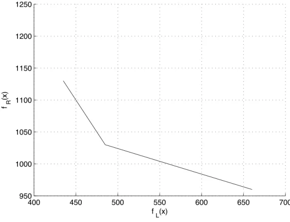
As soon as a solution of the scalarized problem (with a xed α-cut) depends on a parameter λ, a variation of λ ∈ [0,1] gives the optimal solution points. The set of those points then represents a subset of a Pareto set. This is explained with the illustrative example, given in Section 4.2.
Clearly, the approach of partial ordering the intervals may lead to situations of inde-cisiveness (Sengupta and Pal (2000)). This reects the incomparability of the elements of the set of Pareto optimal solutions of the biobjective optimization problem. The com-putation of all such solutions is the basis of our approach to compute the membership function values of the solutions of the initial fuzzy optimization problem. For this, we have to compute the membership function values for all feasible points with the presented in this Chapter method.
As soon as our method is based on optimality conditions for the fuzzy linear optimization problem, we derive them in Section 4.3.
A procedure of computation the membership function value of each element of the fuzzy solution is based on these optimality conditions and is described in Section 4.4. For brevity, the discussions are limited to one element of the set of fuzzy optimal solutions,
but can easily be extended.
The procedure is numerically solved for the wide class of triangular fuzzy numbers (that can be extended to the class of LR-numbers) in Subsection 4.4.1.
This Chapter is concluded with a numerical example where the crucial elements of the fuzzy optimal solution are compared with respect to the membership function values and to objective function value, as well. Of course, the method provides the decision-maker with important quantitative information. These discussions are presented in Subsection 4.4.2.
4.1 Main approach
The linear case of fuzzy optimization problem (3.3) is represented by the following pro-gramming problem with fuzzy coecients in the objective function:
ec >x →min Ax≤b x≥0 (4.1) with ann-dimensional vector of decision variables x.
Here
• ec∈F
n is a vector of fuzzy numbers;
• A ∈Rm×n is the constraint matrix;
• b ∈Rm is the right-hand side vector.
For simplicity instead of problem (4.1) we investigate the fuzzy linear optimization problem ec >x→min Ax=b x≥0. (4.2) Adding slack variables, the investigation of this special problem is of no loss of generality. This problem is replaced with the minimization of the α-cut on the feasible set (see e.g. Chanas and Kuchta (1994, 1996b); Rommelfanger et al. (1989); Zimmermann (1991)).
Thereby, the interval optimization problem is obtained: [c>L(α)x, c>R(α)x]→min
Ax=b x≥0.
(4.3) Using Denition 2.14, the task of nding an optimal solution of interval optimization problem (4.3) reduces to the search of a solution of the following biobjective optimization problem with a xed α-cut:
c>L(α)x→min c>R(α)x→min
Ax=b x≥0.
(4.4)
Optimal solutions of problem (4.4) are dened by means of the Pareto optimality con-cept:
4.1 Main approach 29
Denition 4.1. A feasible point bx ∈X := {x: Ax = b, x ≥ 0} is called Pareto optimal
for linear biobjective optimization problem (4.4) if there does not exist another feasible point xˇ ∈ X such that c>L(α)ˇx ≤ c>L(α)xb and c>R(α)ˇx ≤ c>R(α)bx with at least one strong inequality.
Let Ψ(α) denote the set of Pareto optimal solutions of biobjective optimization prob-lem (4.4) for a certain α-cut.
Such an approach gives no unique optimal solution of the fuzzy optimization problem, since the Pareto optimal solutions of problem (4.4) form a certain set in Rn. According
to Ehrgott (2005) and Zadeh (1963), to compute all Pareto optimal solutions of linear biobjective optimization problem (4.4) it is sucient to compute all optimal points of the linear scalarized problem
λc>L(α)x+ (1−λ)c>R(α)x→min Ax =b
x≥0
(4.5) with 0 < λ < 1. For a xed α-cut the optimal points of problem (4.5) form the sets of optimal solutionsΨα(λ).
This λ can be explained referring to the decision rule of Hurwicz. The optimism / pes-simism parameterλreects the attitude of the decision-maker. Because of this restriction for λ, the weighted sum λc>L(α)x+ (1−λ)c>R(α)x is a convex combination of the objec-tive functions c>L(α)x and c>R(α)x. Therefore, the weighting factor λ can be interpreted as the relative importance between two objective functions of biobjective optimization problem (4.4).
In general, each single optimization problem (4.5) for some xed α and λ determines an optimal solution set. The weighted sum method changes weights among the objective functions c>L(α)x and c>R(α)x systematically (e.g. by a predetermined step size in the hyper-ellipse approximation of Fadel and Li (2002); Li e