Sentiment Analysis on Twitter
by
Rocco Proscia
Supervised by
Jose Luis Balcazar , Marta Arias (LARCA Research Group) Company: ServiZurich
Master in Innovation and Research in Informatics Specialization in Data Mining and Business Intelligence
Facultat d’Informatica de Barcelona (FIB)
Abstract
Master in Innovation and Research in Informatics Specialization in Data Mining and Business Intelligence
Facultat d’Informatica de Barcelona (FIB)
In recent years more and more people have been connecting with Social Networks. One of the most used is Twitter. This huge amount of information is attracting the interest of companies. One reason is that this huge source of information can be used to detect public opinion about their brands and thus improve their business values.
In order to transform the information present in the Social Networks into knowledge several steps are required. This project aim to describe them and provide tools that are able to perform this task.
The first problem is how to retrieve the data. Several ways are available, each one with its own pros and cons. After that it is necessary to study and define proper queries in order to retrieve the information needed.
Once the data is retrieved you may need to filter and explore your data. For this task a Topic Model Algorithm ( LDA ) has been studied and analyzed. LDA has shown positive results when it is tuned in the proper way and it is combined with appropriate visualization techniques. The difference between a Topic Model Algorithm and other Clustering/Segmentation techniques is that Topic Models allows each ”document” ( instance ) to belong to more than one topic ( cluster ).
LDA doesn’t natively work well on Twitter due to the very short length of the tweets. An investigation in the literature has revealed a solution to this problem. Another problem that is common in clustering is how to validate the Algorithm and how to choose the proper number of topics ( clusters), for this problem several metrics in the literature have been explored.
Afterwards, Sentiment Analysis techniques can be applied in order to measure the opin-ion of the users . The literature presents several approaches and ways to solving this problem. This work is focused in solving the Polarity Detection task, with three classes , so, classify if a tweet express a positive , a negative or a neutral sentiment. Here reach accurate results can be challenging, due to the messy nature of the twitter posts. Several approaches have been tested and compared. The baseline method tested is the use of sentiment dictionaries, after that , since the real sentiment of the twitter posts is not available, a sample has been manually labeled and several Supervised approaches combined with various Feature Selection/Transformation techniques have been tested. Finally, a totally new experimental approach, inspired from the Soft Labeling technique present in the literature, has been defined and tested. This method try to avoid the costly task to manually label a sample in order to validate a model. In the literature this problem is solved for the two-class problem, so by considering only positive and negative tweets. This work try to extend the soft-labeling approach to the three class problem.
Alla fine questo Master ´e giunto al termine. Due anni passati in un batter d’occhio in cui ho imparato tantissimo e vissuto le pi´u assurde esperienze, ho avuto la possibilit´a di frequentare un Universit´a fantastica, piena di studenti e professori validi e motivati, in una citt´a folle e meravigliosa come Barcellona.
Vorrei ringraziare inanzitutto i miei genitori per aver permesso ( finanziato ) questa esperienza e i miei due supervisori di tesi Prof. Jose Balcazar e Marta Arias ( ancora auguri per la piccola! ) per avermi sopportato in questi ultimi mesi.
Grazie anche a tutta la gente che , anche solo di passaggio, ho avuto modo di incontrare e passare dei bei momenti, un ringraziamento e saluto , in particolare , anche a chi ´e lontano, ma resta ancora vicino.
E poi basta fare gli sdolcinati che ´e gi´a assai, andiamo a presentare st´o progetto v´a!
Abstract i
Acknowledgements iii
List of Figures vi
List of Tables vii
1 Introduction 1
2 Background Theory 3
2.1 Retrieving Data from the Web . . . 3
2.1.1 API . . . 4
2.1.2 Web Scraping . . . 4
2.1.3 Discussion: Legitimacy of Web Scraping . . . 4
2.2 Storing The Data . . . 8
2.2.1 MongoDB . . . 8
2.3 Information Filtering . . . 9
2.3.1 Topic Modeling . . . 9
2.3.1.1 LDA. . . 10
2.4 Natural Language Processing . . . 13
2.4.1 Structure Analysis and Tokenization . . . 13
2.4.2 Stopwords removal . . . 13
2.4.3 Stemming and Lemmatization . . . 13
2.4.4 Parts of Speech . . . 14
2.4.5 Dependency Parsing . . . 14
2.5 Feature Selection . . . 15
2.5.1 Theχ2 test . . . 16
2.5.2 Information Gain . . . 16
2.6 Supervised Machine Learning . . . 17
2.6.1 The Naive Bayes Classifier . . . 18
3 State of the Art 20 3.1 Topic Modelling on Microblogs . . . 20
3.2 Validation of Topic Models . . . 22
3.3 Visualization of Topic Models . . . 25
3.4 Sentiment Analysis on Microblogs . . . 29 iv
3.5 Lexicons for Sentiment Analysis. . . 30
3.6 Soft Labeling on Microblogs . . . 31
3.7 Probability Calibration of Machine Learning Models . . . 31
4 First Experiment - Information Retrieval 35 4.1 Retrieve the data from Twitter . . . 35
4.2 Information Filtering . . . 35
4.2.1 Exploratory Analysis of The Specific Corpus . . . 36
4.2.2 Application of the LDA . . . 38
4.2.3 Tuning LDA hyperparameters. . . 41
4.2.4 Interpretation of the topics obtained . . . 43
4.2.5 Final Filter . . . 46
5 Second Experiment - Sentiment Analysis 47 5.1 Experiment with Sentiment dictionaries . . . 47
5.2 Negation Detection . . . 48
5.3 Experiment with manually annotated training . . . 48
5.4 Experiment with Soft Labeling . . . 51
5.4.1 Computational Limits . . . 51
5.4.2 Pre-processing . . . 52
5.4.3 Experimental Setup and Results . . . 52
6 Business Insights and Data Visualization 55 6.1 Customers Opinion . . . 55
6.2 Comparison with competitors and future works . . . 57
7 Conclusions 59 7.1 Future Works . . . 60
A Sentiment Analysis - Validation Results 61
B Sentiment Analysis with Soft Labeling - Full Results 64
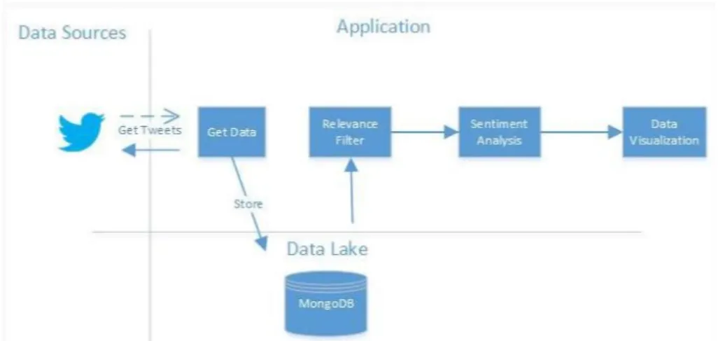
1.1 Project overview . . . 2
2.1 Web Crawling - History of Court Cases . . . 8
2.2 The intuition behind LDA . . . 10
2.3 A Graphical Model representation of the LDA. . . 11
2.4 The role of the αparameter in LDA . . . 12
2.5 A Dependency Tree . . . 15
3.1 Comparison of metrics for LDA . . . 23
3.2 Another comparison of metrics for LDA . . . 25
3.3 Output of LDA, an example . . . 25
3.4 Example of Stacked Bar Chart . . . 26
3.5 Example of Heatmap . . . 27
3.6 Example of Topic-words Association . . . 27
3.7 Example of LDAvis. . . 28
3.8 Another example of LDAvis . . . 29
3.9 Performance of Several Lexicon methods for Sentiment Analysis . . . 30
3.10 Performance of Supervised methods for Sentiment Analysis . . . 30
3.11 Comparison of Probabilistic Predictions . . . 32
3.12 SVM with probability calibration . . . 33
3.13 Gaussian Naive Bayes with probability calibration . . . 34
4.1 Relevant Corpus - Distribution over time . . . 37
4.2 Most Frequent authors in the Relevant Corpus . . . 38
4.3 LDA model Validation - n of topics . . . 40
4.4 LDA model Validation - α and η parameters . . . 41
4.5 Comparison of Two LDA Models . . . 42
4.6 Final LDA Model visualized . . . 43
5.1 Negation Detection with Stanford Dependency Parser . . . 48
5.2 Sentiment Analysis - Class Distribution . . . 49
5.3 The intuition behind soft-label for a 3 classes problem . . . 51
5.4 Soft Labeling approach - results . . . 53
5.5 Calibration Results . . . 54
6.1 Distribution of the customers tweets over time . . . 55
6.2 Sentiment Pie charts and WordClouds . . . 56
6.3 Comparison of the presence of different companies on Twitter . . . 57
6.4 Who talk about insurance companies? . . . 58 vi
2.1 Example of POS tags . . . 14
4.1 Queries Performed on Twitter . . . 36
4.2 A sample of the tweets included in the ’Relevant’ Corpus . . . 38
4.3 Example of the pre-processing used for LDA. . . 39
4.4 First attempts with LDA . . . 39
4.5 Validation for the Final Relevance-Filter Model . . . 46
5.1 Sentiment Analysis with Dictionaries - Results . . . 47
5.2 Sentiment Analysis with manually annotated corpus - polynomial models results . . . 49
5.3 Sentiment Analysis with manually annotated corpus - best models . . . . 50
5.4 Confusion Matrix of the best model. . . 50
5.5 Queries Performed for the Soft-Labeling approach . . . 51
5.6 Some of the negation tokens for Soft Labeling . . . 52
A.1 Sentiment Analysis with manually annotated corpus - results . . . 63
B.1 Models performed on the corpus ”product OR service” - unigrams . . . . 64
B.2 Models performed on the corpus ”product OR service” - bigrams . . . 65
B.3 Models performed on the generic corpus - unigrams. . . 65
B.4 Models performed on the generic corpus - bigrams . . . 65
Introduction
This work is organized as follows. Chapter 2 outlines a theoretical baseline necessary for understanding the following chapters. It describe how to retrieve and store data from Twitter or other Social Networks ( the approach can also be applied to other domains ). After retrieving the information you may need to clean and explore it. For this reason I describe some fundamental Natural Language Processing concepts and Topic Models algorithms. After that, for performing Sentiment Analysis you may need to apply Supervised Algorithms. A brief description of that is proposed with one example: The Naive Bayes Classifier. Before applying any Machine Learning Methods is important to follow the Natural Language pre-processing steps already described, but also apply Feature Selection Techniques, they are briefly described with a couple of examples: the χ2 test and Information Gain.
Chapter 3 represents the theoretical research for this project. The state of the art solutions to the two main problems of the project are described: Topic Model Algorithm and Sentiment Analysis. Both are specific to the Microblogs Environment since our work is based on Twitter and in Twitter the posts are expressed in 140 characters or less. A deep search in the literature has been performed in order to describe the actual state of the art of this area. The length is not the only problem, in fact a tweet is usually messy, with a lot of slang expressions and misspelled words. All these aspects can make life difficult to a Data Scientist and make works terribly techniques that are known to perform well on more ”clean” and ”long” documents. For this reason this Chapter focus on the State of the Art techniques that aims to deal with this domain.
Then Chapter 4 and 5 are dedicated to the experimental part. The first experiment regards Information Retrieval. For this Topic Model Algorithms have shown good results when they are tuned in the proper way, validated with the proper metrics, and visualized with appropriate techniques.
The second experiment deals with Sentiment Analysis, in particular it focuses on the polarity detection task. Here Several approaches have been compared. The most simple just make use of sentiment dictionaries, it represents the baseline for more sophisticated methods. After that a training set is manually labeled and several approaches are performed on it. Finally a new approach has been tested. It is inspired from the techniques of Soft-Labeling, that has shown positive results in several examples in the literature. This experiment try to extend this approach to the three class problem. Finally on the Chapter 6 there are some visualization and insights obtained from the analysis , plus several ideas for future works.
Below is shown an overview of the macro-components of the project.
Background Theory
2.1
Retrieving Data from the Web
The Web is a huge repository of data. It is estimated that the 90% of the worlds data has been generated in the past 2 years. 1 This is a huge opportunity for researchers. Data can be obtained without the cost of performing questionnaires, surveys , interviews or other traditional ways of collecting data .
But the data on the Web is not ready to be analyzed. It is important to know how to extract and clean it. Furthermore not all the data sources can be used without limits. Some companies are not happy to share their data with everyone. In other cases your data may contain sensitive information ( for example in the medical domain ). So in order to respect privacy it is important to anonymize [1] the data before performing any kind of analysis.
So it is important to know which data you are allowed to extract and what you are allowed to do with them.
You can extract data in several ways, they can be placed into three categories:
• Get the data trough an API .
• Use a Web Scraper to crawl the Web.
• Buy the data from a reseller.
The first two approaches are described in the following sections. Nevertheless it is not always possible to retrieve the data trough these techniques. Sometimes the data owners
1
https://www.sciencedaily.com/releases/2013/05/130522085217.htm
can be very conservative and the only way to retrieve your data would be to buy them through an official reseller.
2.1.1 API
Although various APIs exist for a variety of different software applications, in recent times API has been commonly understood as meaning web application API. Typically, a programmer will make a request to an API via HTTP for some type of data, and the API will return this data in the form of XML or JSON. Although most APIs still support XML, JSON is quickly becoming the encoding protocol of choice.
Sometimes the amount of information that you can retrieve with API is limited. Twitter for example limits the number of queries you can perform in a window of 15 minutes 2. Not only the bandwidth is limited but also the amount of information that you can retrieve. The API.search for example, allows to search tweet by a keyword. The problem is that the results are limited to the last 7 days. 3
2.1.2 Web Scraping
In theory, web scraping is the practice of gathering data through any means other than a program interacting with an API (or, obviously, through a human using a web browser). This is most commonly accomplished by writing an automated program that queries a web server, requests data (usually in the form of the HTML and other files that comprise web pages), and then parses that data to extract needed information. In practice, web scraping encompasses a wide variety of programming techniques and technologies, such as data analysis and information security . These books are very exhaustive guides on the topic [2] [3] .
There are several real-world use cases in the market where Web Scraping is used right now. For example e-commerce sites use it to identify best-selling products , job-search sites scrape job listings from several sources, as well as flight-comparison websites search the best flight option through a huge number of airlines and the list can continue.
2.1.3 Discussion: Legitimacy of Web Scraping
Web Scraping is a very powerful technique in order to obtain information at a low cost . However it is important to use it in a conscious way. Most of the times Web Scraping is
2
https://dev.twitter.com/rest/public/rate-limiting
perfectly legal, but there are some cases where it is not. Big companies use web scrapers for their own gain but don’t want others to use bots against them. It is difficult to define precisely what is allowed and what is not because there are several factors to consider. From the law of a specific state , to the Terms of Service (ToS) of a specific Web-Service, if the ToS can be applied to your scraper or not, the type of business you want to perform with the data extracted and so on.
Several article on the web have dealed about the legality of web-scraping4 ,5 ,6 ,7 ,8 ,9. Below some interesting lawsuits are showed.
• Facebook v. Power.com - 2009
Power.com tried to aggregate various social networking accounts in a single place, so you could manage them all at once through a single interface. Yet Facebook charged the company with all sorts of complaints, including copyright and trade-mark infringement, unlawful competition and violation of the computer fraud and abuse act. Power.com asked for the case to be dismissed, but at the end the judge sided with Facebook, but did so in a troubling way, by basically suggesting that since Facebook’s terms of service prohibited these uses, it made it copyright infringement.
The court found that even though the data being used by Power.com isn’t owned by Facebook (it’s the users’) the scraping was still copyright infringement, because in order to scrape the non-infringing content, Power.com had to first ”scrape” the whole page .
This lawsuit has sparked a lot of discussions on the Web. First of all: just because the terms of service said you can’t do any automated scraping of the site, the scrape becomes illicit? Also, they have stated the scrape as copyright infringement just because the scraper had to first read through copyrighted content to get to the non-infringing stuff. But, that seems to go against the entire purpose of copyright law. The fact that the scraper reads copyrighted content shouldn’t mean that it’s infringement. It’s not doing anything with that content other than using it to find the content it can make use of.
• QVC v. Resultly - 2014 4http://www.integrity-research.com/mitigating-risks-associated-with-web-crawling/ 5 http://www.bna.com/legal-issues-raised-by-the-use-of-web-crawling-and-scraping-tools-for-analytics-purposes 6 http://blog.icreon.us/advise/web-scraping-legality 7https://www.techdirt.com/articles/20090605/2228205147.shtml 8 http://www.forbes.com/sites/ericgoldman/2015/03/24/qvc-cant-stop-web-scraping/ #7f2a198c4403 9 http://www.law360.com/articles/389930/collegesource-s-ip-contract-suit-against-rival-tossed
QVC is a well-known TV retailer. Resultly is a start-up shopping app self-described as ”Your stylist, personal shopper and inspiration board” Resultly builds a catalog of items for sale by scraping many online retailers, including QVC. Scraping of retailers websites isn’t unusual; as the court say, ”QVC allows many of Resultlys competitors, e.g., Google, Pinterest, The Find, and Wanelo, to crawl its website.” Resultly cashes in when users click on affiliate links to QVC products .
In May 2014, Resultly’s automated scraper overloaded QVC’s servers, causing outages that allegedly cost QVC $2M in revenue. QVC eventually blocked access to Resultly’s scraper. Subsequent discussions were irresolute, and QVC sought a preliminary injunction based on the Computer Fraud & Abuse Act . The court concludes that QVC hasn’t shown a likelihood of success because Resultly lacked the required intent to damage QVCs system
The outcome of this lawsuit is completely different from the previous one. In this case, even a massive activity of Scraping that has caused the cessation of a service ( not that far from a Denial of Service attack ) has been considered completely legal.
• Collegesource v. AcademyOne - 2015
CollegeSource and AcademyOne are competitors in the market that helps prospec-tive students with the college transfer process. CollegeSource maintain its principal place of business in California, while AcademyOne maintained its principal place of business in Pennsylvania. However, both companies seek to serve the transfer market online not bound by state or region. Important to the appeal, AcademyOne targeted prospective transfer students by state through use of Google AdWords, so-licited California colleges and state educational agencies through phone and email, and sponsored the keynote speaker at a conference held for the benefit of higher education executive officers meeting in San Diego.
CollegeSource claimed to own and copyright a digital collection of 44,000 course catalogs from 3,000 colleges, worth allegedly $10 million. The complete digital col-lection was available through subscription as .pdf files on CollegeSource’s websites. Known to CollegeSource, many of the .pdf files were also individually distributed across thousands of institutional websites. AcademyOne, a few months after its founding, made several attempts to inquire about CollegeSource’s collection of course catalogs as it researched how to compile a nationwide database of college and university level courses to support its college transfer websites. At least three employees registered for trial membership with CollegeSource that allowed them to download three sample catalogs each. CollegeSource declined AcademyOne’s early attempts to partner to keep its competitive advantage in the market place.
Therefore, AcademyOne decided to collect and build its own collection of college and university catalogs to harvest the course information. AcademyOne hired a China-based contractor to collect the catalogs and mine the course descriptions from the files or web pages. The contractor collected over 18,000 .pdf files and thousands of html pages containing course descriptions from a list of schools web-sites that AcademyOne had provided. During this process, the contractor collected roughly 680 .pdf files that contained CollegeSources splash page and copyright page. CollegeSource also claimed some courses descriptions displayed on Acade-myOne’s websites were mined and traceable to CollegeSource’s electronic catalog versions because they supposedly contained typographical errors and ”seeds” intro-duced by the digitization and conversion effort from years prior. Moreover, some of the course catalog pdf files included a page terms prohibiting redistribution, mod-ification, or commercial use of the catalogs ( without consent of CollegeSource) on the second page of the pdf.
The federal judge dismissed claims against AcademyOne by rival CollegeSource over republishing course catalogs and course information digitized and maintained by the latter company, finding that the usage violated neither trademarks nor contracts governing AcademyOne’s subscription service. The judge emphasized that AcademyOnes efforts to collect the information did not run afoul of any contracts established between the two.
• Final Considerations
These lawsuits show that the threshold between allowed and not allowed is very tiny and fragile. The Facebook case shows that scraping by using a user credential is not allowed if the term of service of the platform forbids it.
The second case shows that as long as you allow Web Scraping on your Website, even a heavy scrape that could potentially cause the interruption of your service is not considered as harmful ( as long as it is non intentional ).
Finally the third case show that even a heavy scrape activity that aim to obtain a huge amount of information is not considered illegal as long as there is no agreement between the two counterparts that explicitly forbids it.
If you are interested in going deeper in the argument, this infographic show a wide historical picture of past Court Cases. This section should not be taken as legal council. If you are interested in doing business that involves Web Scraping you should seek for legal advice in order to be sure what you are allowed to do.
Figure 2.1: Web Crawling - History of Court Cases , source: http://www.integrity-research.com/
2.2
Storing The Data
In the Information Retrieval phase, the data needs to be stored somewhere in order to be analyzed later. In this project we have choosen a NoSQL Database for this task. The reason is that we were not aware of the size of the data that we were going to analyze. Thus NoSQL engines provides more scalability in case the size of the data would be very big.
2.2.1 MongoDB
MongoDB is One of the most popular document stores. It is a document oriented database. All data in mongodb is treated in JSON/BSON format. It is a schema less database which goes over tera bytes of data in database. It also supports master slave replication methods for making multiple copies of data over servers making the integration of data in certain types of applications easier and faster. MongoDB combines the best of relational databases with the innovations of NoSQL technologies, enabling engineers to build modern applications. MongoDB maintains the most valuable features of relational databases: strong consistency, expressive query language and secondary indexes. As a result, developers can build highly functional applications faster than NoSQL databases. MongoDB provides the data model flexibility, elastic scalability and
high performance of NoSQL databases. As a result, engineers can continuously enhance applications, and deliver them at almost unlimited scale on commodity hardware. 10
2.3
Information Filtering
Once the data is retrieved, it is a good idea to start exploring the data, in order to check the quality of your data and eventually filter the one that is non relevant for the analysis. If the data is numerical or categorical, traditional techniques from the Multivariate Analysis are suitable for the task. However these techniques could be unsuitable for contents expressed in natural language. Topic Model algorithms can help in this case.
2.3.1 Topic Modeling
Topic models are algorithms for discovering the main themes that pervade a large and otherwise unstructured collection of documents. Topic models can organize the collection according to the discovered themes. Topic modeling algorithms can be applied to massive collections of documents.Recent advances in this field allow us to analyze streaming collections, like you might find from a Web API. Topic modeling algorithms can be adapted to many kinds of data. Among other applications, they have been used to find patterns in genetic data, images,and social networks. [4]
Some general but useful suggestions from [5]:
• Work preferably on a large Corpus.
Topic modeling is built for large collections of texts. In general is recommended to have at least 1,000 items in the collection to model. The question of ”how big” or ”how small” is ultimately subjective.
• Familiarity with the corpus.
This may seem counter intuitive when is planned to use topic modeling to help find out more about a large corpus, and yet it is very important to have at least an idea of what should be there. Topic modeling is not an exact science by any means. The only way to know if the results are useful or wildly off the mark is to have a general idea of what should be there. Most people would probably spot the outlier in a topic of ”tobacco, farm, crops, navy” but more complex topics might be less obvious.
10
https://www.linkedin.com/pulse/real-comparison-nosql-databases-hbase-cassandra-mongodb-sahu
• A way to understand the results.
Topic modeling output is not entirely human readable. One way to understand what the program is telling you is through a visualization, but is important to know how to understand the visualization. Topic modeling tools are fallible, and if the algorithm isn’t right, they can return some bizarre results.
2.3.1.1 LDA
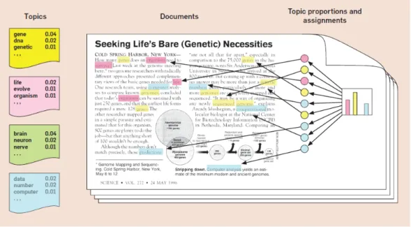
Latent Dirichlet allocation (LDA) is a generative probabilistic model for collections of discrete data such as text corpora. The intuitive idea behind it is the following [6] :
Figure 2.2: The intuition behind LDA , source : www.cs.princeton.edu/~blei/ kdd-tutorial.pdf
In the picture are described the three fundamental components of LDA:
• Each Topicis a distribution over words.
• Each Documentis a mixture of corpus-wide topics.
• Each Word is drawn from one of those topics.
In LDA, the observed data are the words of each document and the hidden variables rep-resent the latent topical structure, i.e., the topics themselves and how each document exhibits them. Given a collection, the posterior distribution of the hidden variables given the observed documents determines a hidden topical decomposition of the collec-tion. Applications of topic modeling use posterior estimates of these hidden variables to perform tasks such as information retrieval and document browsing.
The interaction between the observed documents and hidden topic structure is manifest in the probabilistic generative process associated with LDA, the imaginary random pro-cess that is assumed to have produced the observed data. LetKbe a specified number of topics, V the size of the vocabulary, Dthe number of documents,~αa positive K-vector and η a scalar. Let Dirk(η) denote a K dimensional symmetric Dirichlet with scalar
parameterη .
1. For each topic,
(a) Draw a distribution over words β~k∼Dirv(η) .
2. For each document,
(a) Draw a vector of topic proportions~θd∼Dir(α) .
(b) For each word,
i. Draw a topic assignmentZd,n∼M ult(~θd), Zd,n∈ {1, .., K}
Figure 2.3: A Graphical Model representation of the LDA. Nodes denote random
variables; edges denote dependence between random variables. Shaded nodes denote observed random variables; unshaded nodes denote hidden random variables. The
rectangular boxes are plate notation, which denote replication.
The parameters of the prior are called hyperparameters. So, in LDA, both topic dis-tributions, over documents and over words have also correspondent priors, which are denoted usually withα andη, also because are the parameters of the prior distributions are called hyperparameters.
For the symmetric distribution, a high α value means that each document is likely to contain a mixture of most of the topics, and not any single topic specifically. A low α value puts less such constraints on documents and means that it is more likely that a document may contain mixture of just a few, or even only one, of the topics. Likewise, a highη value means that each topic is likely to contain a mixture of most of the words, and not any word specifically, while a low value means that a topic may contain a mixture of just a few of the words.
Figure 2.4: The role of theαparameter for the symmetric distribution. Each triangle
represent an example of a 3 dimensional topic space. In the first triangle the points represents documents: the red one is 100% of topic C and the blue one is made of 50% of the topic A and 50% of the topic C. The second triangle represent a situation where there is an high value ofα, the documents will be more concentrated on the center so, they will be a mixture of most of the topics. In the last figure is represented a value of
alpha very low, this will bring the documents to began to few topics or only one.
If, on the other hand, the distribution is asymmetric, a highαvalue means that a specific topic distribution (depending on the base measure) is more likely for each document. Similarly, high η values means each topic is more likely to contain a specific word mix defined by the base measure.
In practice, a high α value will lead to documents being more similar in terms of what topics they contain. A high beta-value will similarly lead to topics being more similar in terms of what words they contain.
2.4
Natural Language Processing
Once the data is retrieved and cleaned, is ready to be analyzed. Dealing with document in natural language require specific techniques. Here are defined some concepts that will be useful for understand the next chapters. Some definitions are taken from [7] and [8] which I suggest the reading if interested in knowing more.
2.4.1 Structure Analysis and Tokenization
In this first step, documents are parsed so as to recognize their structure (title, abstract, section, paragraphs). For each relevant logical structure, the system then segments sentences into word tokens (hence the term tokenization). This procedure seems rela-tively easy but (a) the use of abbreviations may prompt the system to detect a sentence boundary where there is none, and (b) decisions must be made regarding numbers, special characters, hyphenation, and capitalization. In the expressions dont, Id, Johns do we have one, two or three tokens? In tokenizing the expression Afro-American, do we include the hyphen, or do we consider this expression as one or two tokens? For numbers, no definite rule can be found. We can simply ignore them or include them as indexing units. An alternative is to index such entities by their type, i.e., to use the tags date, currency, etc. in lieu of a particular date or amount of money. Finally, uppercase letters are lowercased. Thus, the title Export of cars from France is viewed as the word sequence export, of, cars, from, and france.
2.4.2 Stopwords removal
Very frequent word forms (such as determiners the, prepositions from, conjunctions and, pronouns you and some verbal forms is, etc.) appearing in a Stopword list are usually removed. Stopwords, also called empty words as they usually do not bear much meaning, represent noise in the retrieval process and actually damage retrieval performance, since they do not discriminate between relevant and non-relevant documents. Secondly be-cause removing Stopwords allows one to reduce the storage size of the indexed collection, hopefully within the range of 30% to 50%.
2.4.3 Stemming and Lemmatization
Stemming and Lemmatization are the basic text processing methods for English text. The goal of both stemming and Lemmatization is to reduce inflectional forms and some-times derivationally related forms of a word to a common base form.
However, the two words differ in their flavor. Stemming usually refers to a crude heuristic process that chops off the ends of words in the hope of achieving this goal correctly most of the time, and often includes the removal of derivational affixes. Lemmatization usually refers to doing things properly with the use of a vocabulary and morphological analysis of words, normally aiming to remove inflectional endings only and to return the base or dictionary form of a word, which is known as the lemma . If confronted with the token saw, stemming might return just s, whereas Lemmatization would attempt to return either see or saw depending on whether the use of the token was as a verb or a noun. The two may also differ in that stemming most commonly collapses derivationally related words, whereas Lemmatization commonly only collapses the different inflectional forms of a lemma. 11
2.4.4 Parts of Speech
Part-of-speech (POS) tagging is normally a sentence based approach . Given a sentence formed of a sequence of words, POS tagging tries to label (tag) each word with its correct part of speech (also named word category, word class, or lexical category).
Tag Description JJ Adjective RB Adverb
VB Verb, base form
IN Preposition or subordinating conjunction NN Noun, singular or mass
Table 2.1: Some Part-of-speech tags used in the Penn Treebank Project. The full list is available here: https://www.ling.upenn.edu/courses/Fall_2003/ling001/
penn_treebank_pos.html
For example the sentence ”I like potatoes” tagged with POS become : ”I / PRPlike / VBP potatoes /NNS” .
2.4.5 Dependency Parsing
Syntactic dependency representations of sentences have a long history in theoretical linguistics. Recently, they have found renewed interest in the computational parsing community due to their efficient computational properties and their ability to naturally model non-nested constructions, which is important in freer-word order languages such as Czech, Dutch, and German. This interest has led to a rapid growth in multilingual data sets and new parsing techniques. [9]
11
Figure 2.5: A Dependency Tree
The fundamental notion of dependency is based on the idea that the syntactic structure of a sentence consists of binary asymmetrical relations between the words of the sentence. The idea is expressed in the following way in the opening chapters of Tesnire [1959] :
The sentence is an organized whole, the constituent elements of which are words. [1.2] Every word that belongs to a sentence ceases by itself to be isolated as in the dictionary. Between the word and its neighbors, the mind perceives connections, the totality of which forms the structure of the sentence. [1.3] The structural connections establish dependency relations between the words. Each connection in principle unites a superior term and an inferior term. [2.1] The superior term receives the name governor. The inferior term receives the name subordinate. Thus, in the sentence Alfred parle [. . . ], parle is the governor and Alfred the subordinate. [2.2]
2.5
Feature Selection
Feature selection is also called variable selection or attribute selection.
It is the automatic selection of attributes in your data (such as columns in tabular data) that are most relevant to the predictive modeling problem you are working on.
Feature selection is different from dimensionality reduction. Both methods seek to reduce the number of attributes in the dataset, but a dimensionality reduction method do so by creating new combinations of attributes, where as feature selection methods include and exclude attributes present in the data without changing them.
Examples of dimensionality reduction methods include Principal Component Analysis, Singular Value Decomposition and Sammons Mapping.
Feature selection is itself useful, but it mostly acts as a filter, muting out features that arent useful in addition to your existing features. [10]
2.5.1 The χ2 test
Definition: The Chi-Square Test is the widely used non-parametric statistical test that describes the magnitude of discrepancy between the observed data and the data expected to be obtained with a specific hypothesis.
The observed and expected frequencies are said to be completely coinciding when theχ2 = 0 and as the value ofχ2 increases the discrepancy between the observed and expected data becomes significant. The following formula is used to calculate Chi-square:
χ2 =P(O−E)2 E
Where:
O = Observed Frequency
E = Expected or Theoretical Frequency
The computed value of χ2 is compared with the table value of χ2 for a given degree of
freedom and at a given significance level. If the calculated value exceeds the table value, then the difference between the observed frequencies and expected frequencies is said to be significant, i.e. it could not have arisen due to the fluctuations in simple sampling. The following five basic conditions should be met before applying the chi-square test:
• The observation data must be independent of each other.
• The data should be expressed in original units and not in percentage or ratio form so that it can be easily compared.
• The data must be drawn randomly from the target population.
• The sample should include at least 50 observations.
• Every cell must have five or more observations. Each data entry is called a cell. In case, the observations are less than 5, then the value of χ2 shall be overestimated and will result in the rejection of several Null Hypothesis. 12
2.5.2 Information Gain
Information Gain is frequently employed as a term-goodness criterion in the field of Machine Learning. It measures the number of of bits of information obtained for category prediction by knowing the presence or absence of a term in a document. Letcmi=1 denote
12
the set of categories in the target space. The information gain of term t is defined to be :
G(t) =−Pm
i=1P(ci)log(P(ci))
+P(t)Pm
i=1P(ci|t)log(P(ci|t) +P(¯t))Pmi=1P(ci|¯t)log(P(ci|¯t))
This definition is more general than the one employed in binary classification models. A more general form is used because text categorization problems usually have a m-ary category space( where m may be up to tens of thousands) , and we need to measure to goodness of a term globally with respect to all categories on average. [11]
2.6
Supervised Machine Learning
The aim of supervised, machine learning is to build a model that makes predictions based on evidence in the presence of uncertainty. As adaptive algorithms identify patterns in data, a computer ”learns” from the observations. When exposed to more observations, the computer improves its predictive performance.
Specifically, a supervised learning algorithm takes a known set of input data and known responses to the data (output), and trains a model to generate reasonable predictions for the response to new data.
For example, suppose you want to predict whether someone will have a heart attack within a year. You have a set of data on previous patients, including age, weight, height, blood pressure, etc. You know whether the previous patients had heart attacks within a year of their measurements. So, the problem is combining all the existing data into a model that can predict whether a new person will have a heart attack within a year.
You can think of the entire set of input data as a heterogeneous matrix. Rows of the matrix are called observations, examples, or instances, and each contain a set of measurements for a subject (patients in the example). Columns of the matrix are called predictors, attributes, or features, and each are variables representing a measurement taken on every subject (age, weight, height, etc. in the example). You can think of the response data as a column vector where each row contains the output of the corresponding observation in the input data (whether the patient had a heart attack). To fit or train a supervised learning model, choose an appropriate algorithm, and then pass the input and response data to it.
• In classification, the goal is to assign a class (or label) from a finite set of classes to an observation. That is, responses are categorical variables. Applications in-clude spam filters, advertisement recommendation systems, and image and speech recognition. Predicting whether a patient will have a heart attack within a year is a classification problem, and the possible classes are true and false. Classification algorithms usually apply to nominal response values. However, some algorithms can accommodate ordinal classes.
• In regression, the goal is to predict a continuous measurement for an observation. That is, the responses variables are real numbers. Applications include forecasting stock prices, energy consumption, or disease incidence. 13
2.6.1 The Naive Bayes Classifier
It is a classification technique based on Bayes Theorem with an assumption of inde-pendence among predictors. In simple terms, a Naive Bayes classifier assumes that the presence of a particular feature in a class is unrelated to the presence of any other fea-ture. For example, a fruit may be considered to be an apple if it is red, round, and about 3 inches in diameter. Even if these features depend on each other or upon the existence of the other features, all of these properties independently contribute to the probability that this fruit is an apple and that is why it is known as ’Naive’.
Naive Bayes model is easy to build and particularly useful for very large data sets. Along with simplicity, Naive Bayes is known to outperform even highly sophisticated classification methods. 14
Given a class variableyand a dependent feature vectorx1, ..., xn . Bayes theorem states
the following relationship: P(y|x1, ..., xn) =
P(y)P(x1, ..., xn|y)
P(x1, ..., xn)
Using the naive independence assumption that: P(xi|y, x1, ..., xi−1, xi+1, ..., xn) =P(xi)|y
For allithis relation is simplified to: P(y|x1, ..., xn) = P(y)Qn i=1P(xi|y) P(x1, ..., xn) 13 https://es.mathworks.com/help/stats/supervised-learning-machine-learning-workflow-and-algorithms.html 14 https://www.analyticsvidhya.com/blog/2015/09/naive-bayes-explained/
Since P(x1, ..., xn) is constant given the input, we can use the following classification
rule: ˆ
y=argmaxP(y)Qn
i=1P(xi|y)
And we can use Maximum A Posteriori (MAP) estimation to estimateP(y) andP(xi|
y); the former is then the relative frequency of class y in the training set. 15
15
State of the Art
This Chapter extend the previous one by going deep in several topics. First of all are described the State of the Art techniques that needs to be applied to Topic Model Algorithms for reach satisfactive results.
After that are discussed the state of the art techniques for Sentiment Analysis. The last paragraph, deals about an argument that is used in the last experiment: Probability Calibration. Not all Machine Learning methods offer good probability estimations for their predictions, are discussed methodologies that can help improve the probability estimations.
3.1
Topic Modelling on Microblogs
Twitter, or the world of 140 characters poses serious challenges to the efficacy of topic models on short , messy text. While topic models such as Latent Dirichlet Alloca-tion (LDA) have a long history of successful applicaAlloca-tion to news articles and academic abstracts, they are often less coherent when applied to Microblog contents like Twitter. Several papers are dedicated to this problem and propose various solutions to this. Mehrotra et al. [12] try to obtain better LDA topics without modifying the basic ma-chinery of LDA, in particular they present various pooling schemes to aggregate tweets into ”macro-documents” for use as a training data to build LDA models. The motivation behind tweet pooling is that individual tweets are very short (<= 140 characters) and hence treating each tweet as an individual document does not present adequate term co-occurrence data within documents. Aggregating tweets which are similar in some sense (semantically, temporally, etc.) enriches the content present in a single document from which the LDA can learn a better topic model:
• Author-wise Pooling: Pooling tweets according to author.This method show to be superior to unpooled Tweets. For this method, document for each author is built, which combines all tweets they have posted.
• Burst-score wise PoolingA trend on Twitter (sometimes referred to as a trend-ing topic) consists of one or more terms and a time period, such that the volume of messages posted for the terms in the time period exceeds some expected level of activity. In order to identify trends in Twitter posts, unusual bursts” of term frequency can be detected in the data.We run a simple burst detection algorithm to detect such trending terms and aggregate tweets containing those terms having high burst scores. To identify terms that appear more frequently than expected, we will assign a score to terms according to their deviation from an expected fre-quency. Assume that M is the set of all messages in our tweets dataset, R is a set of one or more terms (a potential trending topic) to which we wish to as-sign a score, and d ∈ D represents one day in a set D of days.We then define M(R;d) as the subset of Twitter messages in M such that (1) the message con-tains all the terms in R and (2) the message was posted during day d. With this information, we can compare the volume in a specific day to the other days. Let M ean(R) = |D1|P
d∈DM(R, d) over the days d∈D. The burst-score is then
defined as:
burst-score(R, d) = |M(R,d)SD(R)−M ean(R)|
• Temporal Pooling: When a major event occurs, a large number of users often start tweeting about the event within a short period of time. To capture such temporal coherence of tweets, the fourth scheme and our second novel pooling proposal is known as Temporal Pooling, where we pool all tweets posted within the same hour.
• Hashtag-based Pooling: A Twitter hashtag is a string of characters preceded by the hash (#) character. In many cases hashtags can be viewed as topical markers, an indication to the context of the tweet or as the core idea expressed in the tweet, therefore hashtags are adopted by other users that contribute similar content or express a related idea. One example of the use of hashtags is ”ask GAGA anything using the tag #GoogleGoesGaga for her interview! RT so every monster learns about it!! ” referring to an exclusive interview for Google by Lady Gaga (singer). For the hashtag-based pooling scheme, we create pooled documents for each hashtag. If any tweet has more than one hashtag, this tweet gets added to the tweet-pool of each of those hashtags.
Ramage et al. [13] use a partially supervised learning model (Labeled LDA) that maps the content of the Twitter feed into dimensions. These dimensions correspond roughly to substance, style, status, and social characteristics of posts. So while the latent dimen-sions in twitter can help identify broad trends, several classes of tweets specific labels are applied to subsets of the posts. For example hashtags ,emoticons and social signals such as replies, mentions ( @user) , questions( ? ) .
3.2
Validation of Topic Models
The validation of the topics obtained with Topic Model can be performed in several ways, by using metrics or by human judgment.
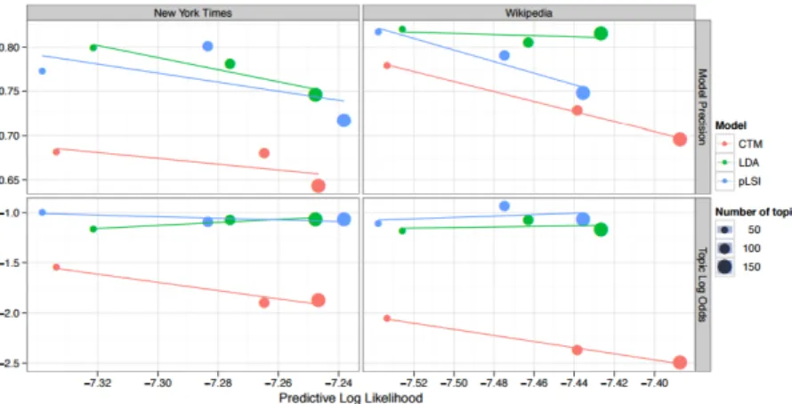
Chang et al. [14] have compared several metrics with human judging techniques. The techniques analyzed are the following:
• Word intrusion: For each trained topic, take the six most probable words, sub-stitute one of them with another, randomly chosen word ( an intruder ) and see whether a human can reliably tell which one it was. If so, the trained topic is topically coherent if not, the topic has no discernible theme . For example, most people readily identify apple as the intruding word in the set {dog, cat, horse, apple, pig, cow}because the remaining words make sense together. While for the set{car, teacher, platypus, agile, blue, Zaire} identifying the intruder is more dif-ficult. This will bring people to choose the intruder at random, implying a topic with poor coherence.
Let wkm be the index of the intruding word generated from the k topic inferred by model m. Let imk,s be the intruder selected by the subject s generated from the topic k inferred by the model s. Be S the total number of subjects. The model precision is defined by the fraction of subjects agreeing with the model: M Pkm =P
s1(imk,s =wmk)/S
• Topic intrusion: Subjects are shown the title and a snippet from a document. Along with the document they are presented with four topics. Three of those topics are the highest probability topics assigned to that document. The remaining intruder topic is chosen randomly from the other low-probability topics in the model. The subject is instructed to choose the topic which does not belong with the document. As before, if the topic assignment to documents were relevant and intuitive, we would expect that subjects would select the topic we randomly added as the topic that did not belong. The topic log odds is defined as a quantitative
measure of the agreement between the model and human judgments on this task. Letdm denote model m’s point estimate of the topic proportions vector associated with document d. Further let jd,sm be the intruding topic selected by subjectsfor documentdon modelmand letjmd denote the ”true” intruder. In other words the topic log odds is the log ratio of the probability mass assigned to the true intruder to the probability mass assigned to the intruder selected by the subject:
T LOdm= (P sθd,jmm d,∗−θ m d,jm d,s)/S
• Log-Likelihood: A predictive metrics. The dataset need to be splitted in training and test. Let bewd the documents in the test set and be the model described by
the topic matrix Φ . The log-likelihood is defined as: L(w) = log p(w|Φ) = P
dlog p(wd|Φ)
• Perplexity It make use of the log-likelihood. Is defined as : perplexity(test set w) = exp−
L(w) PD d=1 PV v=1njv
Which is a decreasing function of the log-likelihood. The lower the perplexity, the better the model.
The paper shows that log-likelihood ( and consequently perplexity ) and human judg-ment is not correlated. Sometimes are also slightly uncorrelated.
Figure 3.1: Comparison of metrics for LDA from Chang et al. . Comparison between
Word Intrusion ( top row ), Topic Intrusion ( bottom row) and the log likelihood. Each point is colored by model and sized according to the number of topics used to fit the model. Each model is accompanied by a regression line. Increasing likelihood does not increase the agreement between human subjects and the model for either task (as
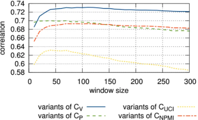
Roder et al. [15] compare other metrics with human judging and some of them seems to be very promising:
• UMass Coherence : Is an asymmetrical confirmation measure between top word pairs ( smoothed conditional probability ). The summation of UMass coher-ence accounts for the ordering among the top words of a topic:
CU M ass= n·(N2−1)PNi=2Pj=1i−1logP(wP(wi,wjj))+
Word probabilities are estimated based on document frequencies of the original documents used for learning the topics.
The main idea of this coherence is that the occurrence of every top word should be supported by every top preceding top word. Thus, the probability of a top word to occur should be higher if a document already contains a higher order top word of the same topic. Therefore, for every word the logarithm of its conditional probability is calculated using every other top word that has a higher order in the ranking of top words as condition. The probabilities are derived using document co-occurrence counts. The single conditional probabilities are summarized using the arithmetic mean.
• UCI Coherence : based on pointwise mutual information, the formula is: CU CI = 2 N ·(N −1) PN−1 i=1 PN j=i+1P M I(wi, wj) P M I(wi, wj) =log P(wi, wj) + P(wi)·P(wj)
The word co-occurrence counts are derived using a sliding window . For every word pair the PMI is calculated. The arithmetic mean of the PMI values is the result of this coherence.
• normalized PMI : vij =N P M I(wi, wj)γ = logP(wi,wj)+ P(wi)·P(wj) −log(P(wi, wj) +) γ
• CV : Is a combination between the indirect cosine measure with the NPMI and the boolean sliding window.
• Direct Coherent Measure ( cp ) : Also this is a combination. It combines
Fitelsons confirmation measure with the boolean sliding window.
The comparison of the metrics is shown in the plot below. The cv metrics is the one
Figure 3.2: Comparison of metrics for LDA from Roder et al.
3.3
Visualization of Topic Models
Interpreting the output of a topic model can be challenging as can be seen in this example.
A huge amount of words concatenated with numbers is not the best way to interpret the results of a model. Below several visualization techniques are proposed in order to improve the interpretability ( They are taken from [16] and [17] ) .
• Stacked Bar Chart
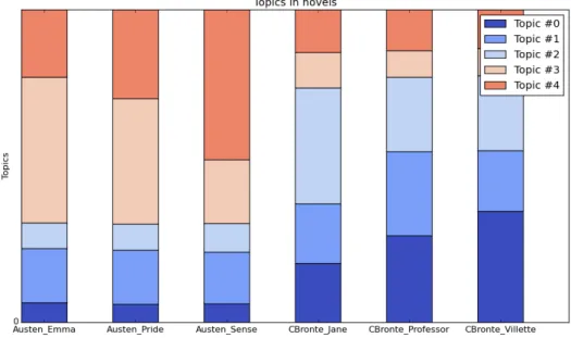
The idea underlying the stacked bar chart is that each text has some proportion of its words associated with each topic. Because the model assumes that every word is associated with some topic, these proportions must add up to one. For example, in a three topic model, text number 1 might have 50% of its words associated with topic 1, 25% with topic 2, and 25% with topic 3. The stacked bar chart represents each document as a bar broken into colored segments matching the associated proportions of each topic. The stacked bar chart below expresses the topic proportions found in the six novels in the austen-bront corpus.
Figure 3.4: A Stacked Bar Chart
• Heatmap
Another useful visualization of topic shares is the heatmap. A heat map (or heatmap) is a graphical representation of data where the individual values con-tained in a matrix are represented as colors.
Figure 3.5: An Example of Heatmap, is visible that topics 3 and 4 are quite correlated with the documents of Austen, while topic 0 and 2 dominates in the CBronte ones
• Topic-words Associations
An alternative to the crude visualization of words and probabilities that is the output of LDA can be to plot the words for each topic . For each topic vary the size of the word based on his weight.
Figure 3.6: Example of Topic-words Association. Is visible that the topic 3 is much
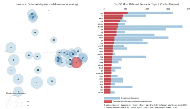
• LDAvis
Last but not the least, a very fascinating library for visualizing topic models. Is available in python 1 and R 2 .
Figure 3.7: Example of LDAvis.
On the left side are represented the first two components of a Principal Compo-nent Analysis performed on the topic space. Each topic is a circle, the biggest is the circle more is representative. On the right side is possible to see the most representative words for this topic. The red bar represent the frequency of the world in the topic while the blue bar represent the frequency of the world in the whole corpus.
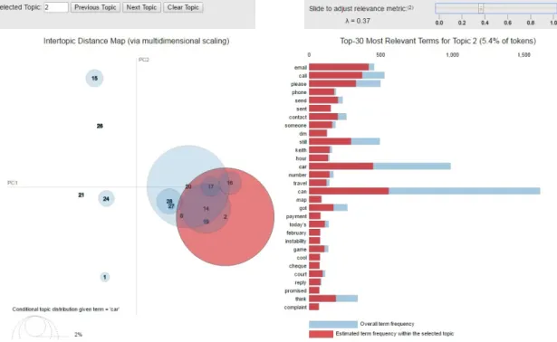
LDAvis allows a very nice interaction with the user, for example in the screen below I have done two things: first I have moved the slide on top and i set λto 0.37, this will makes emerge words that are unique to that specific topic. A too low value forλwill makes emerge stopwords or words that are yes unique for that topic but could be not good for interpreting the topic.
In this second example I have put the mouse on the word”car”. This change the circles area on the map. Now the size of the circle represents how important is the world ”car” for that specific topic.
1
https://pyldavis.readthedocs.io/en/latest/
2
Figure 3.8: Another example of LDAvis.
3.4
Sentiment Analysis on Microblogs
Sentiment analysis is a line of research that combines techniques from various fields such as Natural Language Processing and Machine Learning to extract, from a given piece of text, information on the authors personal impressions.
Several approaches are available, for example Pandey et al [18] divide Sentiment Analysis into two main sub tasks:
• Subjectivity Recognition: which is usually a binary problem that consists in deciding whether a given text contains personal impressions or not.
• Polarity Detection: once obtained the data with personal impressions, try to extract concrete information from the subjective writing.
For the Polarity detection several variants are present in the literature. There is who consider the problem as a binary-problem ( positive or negative ). Some others consider also the neutral class , thus positive , negative and neutral. Some other works ( for example [19] ) try to enlarge the spectrum of the emotions, so not only positive or negative but also happy, unhappy, skeptical and playful.
3.5
Lexicons for Sentiment Analysis
Typically, lexicon-based approaches for sentiment classification are based on the insight that the polarity of a piece of text can be obtained on the ground of the polarity of the words which compose it.
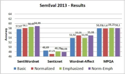
Semeraro et al [20] perform a comparison among several lexicon sources available on the Web. They test the lexicons on Twitter Data. They evaluate four lexicons: Senti-WordNet , Senti-WordNet-Affect , MPQA and SenticNet. They make use of the lexicons in a supervised way. They make use of a labeled training also in order to leverage the weights of the sentiment words. They test several configurations and these are the results.
Figure 3.9: Performance of Several Lexicon methods for Sentiment Analysis from Semeraro et al for the three class problem ( positive , negative and neutral ) performed
on the SemEval 2013 Data [21]
On the same dataset Kolchyna et al [22] perform several approaches. Some includes the use of lexicons and others adopt supervised models. The supervised methods outperform the lexicon ones and their results are the following:
Figure 3.10: Performance of Supervised methods for Sentiment Analysis from Kolchyna et al for the three class problem ( positive , negative and neutral ) performed
on the SemEval 2013 Data
The domain of a lexicon is also important. A word can have a different polarity on different domains. In general statistical and machine
Marquez et al [23] have built a lexicon specific for twitter. They use several seed lexicons in order to extract sentiment words from unlabeled tweets.
3.6
Soft Labeling on Microblogs
Labeling a training set can be costly and time consuming. Thus for the Polarity Detec-tion task on Twitter is common [24] [25] [26] to label the training corpora automatically by using tweets with smileys. So tweets containing happy faces ( :-) , ;) , etc. ) will be used as a positive corpus , while the ones containing sad faces ( :( , :’( , ... ) will constitute the negative corpus.
This approach has shown good results not only in a specific domain but also in the general domain, so even by using a generic domain training corpus is possible to reach good results in a specific domain. However this results are limited to the two class problem. So the sentiment is classified into positive and negative only.
3.7
Probability Calibration of Machine Learning Models
When performing classification you often want not only to predict the class label, but also obtain a probability of the respective label. This probability gives you some kind of confidence on the prediction. Some models gives poor estimates of the class probabil-ities and some even do not not support probability prediction. The calibration module included in the scikit-learn package in Python allows to better calibrate the probabilities of a given model, or to add support for probability prediction.
Below I provide some example of this library in action, everything is taken from the H. Metzen blog [27].
Well calibrated classifiers are probabilistic classifiers for which the output of the pre-dict proba method can be directly interpreted as a confidence level. For instance, a well calibrated (binary) classifier should classify the samples such that among the samples to which it gave a predict proba value close to 0.8, approximately 80% actually belong to the positive class. The following plot compares how well the probabilistic predictions of different classifiers are calibrated:
Logistic Regression returns well calibrated predictions by default as it directly optimizes log-loss. In contrast, the other methods return biased probabilities; with different biases per method:
Figure 3.11: Comparison of Probabilistic Predictions
Naive Bayes (GaussianNB) tends to push probabilities to 0 or 1 (note the counts in the histograms). This is mainly because it makes the assumption that features are conditionally independent given the class, which is not the case in this dataset which contains 2 redundant features.
Linear Support Vector Classification (LinearSVC) shows an even more sigmoid curve as the RandomForest Classifier, which is typical for maximum-margin methods , which focus on hard samples that are close to the decision boundary (the support vectors). Two approaches for performing calibration of probabilistic predictions are provided: a parametric approach based on Platt’s sigmoid model and a non-parametric approach based on isotonic regression (sklearn.isotonic). Probability calibration should be done on new data not used for model fitting. The class CalibratedClassifierCV uses a cross-validation generator and estimates for each split the model parameter on the train samples and the calibration of the test samples. The probabilities predicted for the folds are then averaged. Already fitted classifiers can be calibrated by CalibratedClassifierCV via the parameter cv=”prefit”. In this case, the user has to take care manually that data for model fitting and calibration are disjoint.
The following experiment is performed on an artificial dataset for binary classification with 100.000 samples (1.000 of them are used for model fitting) with 20 features. Of the 20 features, only 2 are informative and 10 are redundant. The figure shows the estimated probabilities obtained with logistic regression, a linear support-vector classifier (SVC), and linear SVC with both Isotonic calibration and Sigmoid calibration. The calibration performance is evaluated with Brier score brier score loss, reported in the legend (the smaller the better).
Figure 3.12: SVM with probability calibration
One can observe here that logistic regression is well calibrated as its curve is nearly diagonal. Linear SVC’s calibration curve has a Sigmoid curve, which is typical for an under-confident classifier. In the case of LinearSVC, this is caused by the margin property of the hinge loss, which lets the model focus on hard samples that are close to the decision boundary (the support vectors). Both kinds of calibration can fix this issue and yield nearly identical results. The next figure shows the calibration curve of Gaussian naive Bayes on the same data, with both kinds of calibration and also without calibration.
Figure 3.13: Gaussian Naive Bayes with probability calibration
One can see that Gaussian naive Bayes performs very badly but does so in an other way than linear SVC: While linear SVC exhibited a Sigmoid calibration curve, Gaussian naive Bayes’ calibration curve has a transposed-Sigmoid shape. This is typical for an over-confident classifier. In this case, the classifier’s overconfidence is caused by the redundant features which violate the naive Bayes assumption of feature-independence. Calibration of the probabilities of Gaussian naive Bayes with Isotonic regression can fix this issue as can be seen from the nearly diagonal calibration curve. Sigmoid calibration also improves the brier score slightly, albeit not as strongly as the non-parametric Iso-tonic calibration. This is an intrinsic limitation of Sigmoid calibration, whose parametric form assumes a Sigmoid rather than a transposed-Sigmoid curve. The non-parametric Isotonic calibration model, however, makes no such strong assumptions and can deal with either shape, provided that there is sufficient calibration data. In general, Sigmoid calibration is preferable if the calibration curve is Sigmoid and when there is few cali-bration data while Isotonic calicali-bration is preferable for non- Sigmoid calicali-bration curves and in situations where many additional data can be used for calibration.
First Experiment - Information
Retrieval
4.1
Retrieve the data from Twitter
The Zurich Insurance Group reside in different country all over the world. Thus different language are used on twitter. This research focus on tweets written in English. When retrieving tweets is possible to filter them by language with the parameter LANG. How-ever still a small subset of tweet written in other languages is retrieved, in particular tweets written in more than one language ( For example : ”Senior Planning Analyst * http:// bit.ly/VmWsX2 * Empresa: Zurich Insurance Company Ltd * Lugar: Zurich #empleo #trabajo #suiza” ) .
Twitter offer an API in order to retrieve information. Several interfaces are available. In order to retrieve tweet by a keyword is possible to use the API.search. In python one way to approach the API is with the Tweepy library1 .
4.2
Information Filtering
The first problem is to formulate proper queries in order to retrieve the data. Intuitively a specific query like ”zurich insurance group” would do the job. However performing a specific query could potentially rule out an important amount of tweet. Twitter is the world where everyone express concepts in 140 characters so it reasonable to think that people would refer to the Zurich group also in other ways. In order to include more cases is possible to make a more generic query like: ”zurich” . The problem of this query is
1
http://www.tweepy.org/
that introduce an enormous amount of noise due to ambiguities. Just think about the city of Zurich, the airport of Zurich and so on . Furthermore Zurich has got several official pages. It is important to individuate them and retrieve the tweets related to them. They are basically of two categories, messages ( @) and hashtags (#).
Finally the following queries has been performed, the results are then combined in order to obtain a ”specific corpus” and a ”generic one”. The tweets obtained below are generated from October 2007 to October 2016
Query Cat. Description Size
1) zurich Gen. tweets that contains
the keyword zurich 1.182.447 2) zurich insurance Spec
tweets that contains the keywords zurich insurance 57.078 3) @zurich OR @zurichinsuk OR @zurichinsider OR @zurichaustralia OR @zurichnanews OR @zurichireland OR @zurichmunicipal OR @zurichcanada
Spec message directed
to the official pages 31.009 4) #zurichinsuk OR
#zurichinsider OR #zurichaustralia OR #zurichnanews OR #zurichireland OR #zurichmunicipal OR #zurichcanada
Spec
tweets that includes the hashtags of the official pages
48
Table 4.1: Queries Performed on Twitter
The corpora obtained are not independent. Most of the tweet obtained in the queries 2, 3 and 4 are subsets of the first one. Also the sets 2 , 3 and 4 are not mutually exclusive and they share several common tweets. Furthermore the the query 4 doesn’t include the hashtag #zurich , because it contains a lot of noise . The first query return as well tweets with the hashtag #zurich .
The size of the first corpus suggest that the generic corpus present an important amount of noise.
4.2.1 Exploratory Analysis of The Specific Corpus
The tweets from the specifics corpora are merged. The redundant tweets are removed. The retweets are also discarded with the following criteria: Consider the following tweets:
• ”I like potatoes”
• ”RT:I like potatoes”
The first retweet doesn’t add any new information, furthermore is just redundant and thus is discarded. The third one add contents to the original tweet, thus is kept. After the merging phase a corpus of 65.504 tweet is obtained. Below the timestamps of the tweets are aggregated by month and the distribution over time is showed. Is visible that until 2012 a very small amount of tweet is published, the trend is growing but very slowly. From 2012 the things start to change. This is because the Zurich Group start join Twitter on this period and begin to create his pages on several countries. The trend keeps growing until the present.
Figure 4.1: Relevant Corpus - Distribution over time
In the histogram are showed the most frequent authors in the relevant corpus. The Zurich pages dominates the rank followed by several news pages and job announces pages. This combined to a quick look on a sample of the corpus suggest that still doesn’t show interesting information. Is true that they deal about the Zurich Group but still doesn’t show the information that interest us. Much effort is required in order to extract relevant information.
Figure 4.2: Most Frequent authors in the Relevant Corpus ’Credit Portfolio Manager: Zurich Insurance Group Location : Milano
LOM IT Zurich is one of the world\xe2\x80\x99s leadin... http:// bit.ly/2dSAgWp’ ’#Jobs #Boston (USA-MA-Boston) Medical Stop Loss Underwriter I:
Zurich Insurance is currently looking for a Me... http:// tinyurl.com/za5bfhf’ ’Zurich Insurance transformation designed from the customer
back #DF16 very #customer -adaptive’
’Great comments from Emma @Zurich at #DF16 about #b2b customers
bringing consumer experience expectations to the workplace. #customerobsessed’ ’Customer stories live at #df16 as #ZurichInsurance transforming
with ZurichFutureYou built on #Salesforce pic.twitter.com/btyfUBl3MH’ ’Cyber security & privacy risks for financial institutions @AccentureSecure @BarclaysUK @CooleyLLP @JonesDay @Zurich http:// bit.ly/2bcsZzo’
’Credit Portfolio Manager: Zurich Insurance Group Location : Milano LOM
IT Zurich is one of the world\xe2\x80\x99s leading... http:// fb.me/47GWKeQt7’
Table 4.2: A sample of the tweets included in the ’Relevant’ Corpus
4.2.2 Application of the LDA
Is difficult to have an idea