CR-LIBM
A library of correctly rounded elementary functions in
double-precision
Catherine Daramy-Loirat, David Defour, Florent de Dinechin,
Matthieu Gallet, Nicolas Gast, Jean-Michel Muller
Important warning
This report describes and proves version 0.10beta of thecrlibmlibrary. It may therefore not correspond to the latest version. An up-to-date version will always be distributed along with the code.
Many thanks to...
• Vincent Lef`evre, from INRIA-Lorraine, without whom this project would’t have started, and who
has since then lended a helpful hand in more than 17 occasions;
• The Ar´enaire project at ´ENS-Lyon, especially Marc Daumas, Sylvie Boldo, Guillaume Melquiond,
Nathalie Revol and Arnaud Tisserand;
• Guillaume Melquiond for Gappa and its first-class hotline; • The MPFR developers, and especially the INRIASPACESproject;
• The Intel Nizhniy-Novgorod Lab, especially Andrey Naraikin, Sergei Maidanov and Evgeny
Gvozdev;
• The contributors of bits and pieces, Phil Defert and Eric McIntosh from CERN, Patrick Pelissier
from INRIA.
• All the people who have reported bugs, hoping that they continue until they have to stop: Evgeny
Gvozdev from Intel with special thanks, Christoph Lauter from TUM ¨unchen, Eric McIntosh from CERN, Patrick Pelissier and Paul Zimmermann from INRIALorraine.
• William Kahan at UCBerkeley, Peter Markstein at HP, Neil Toda at Sun, Shane Story at Intel, and
many others for interesting and sometimes heated discussions.
• Serge Torres for LIPForge
Contents
0 Getting started with crlibm 7
0.1 What iscrlibm? . . . 7
0.2 Compilation and installation . . . 7
0.3 Usingcrlibmfunctions in your program . . . 8
0.4 Currently available functions . . . 8
0.5 Writing portable floating-point programs . . . 8
1 Introduction: Goals and methods 11 1.1 Correct rounding and elementary functions . . . 11
1.2 A methodology for efficient correctly-rounded functions . . . 11
1.2.1 The Table Maker’s Dilemma . . . 11
1.2.2 The onion peeling strategy . . . 12
1.3 The Correctly Rounded Mathematical Library . . . 12
1.3.1 Two steps are enough . . . 12
1.3.2 Portable IEEE-754 FP for a fast first step . . . 13
1.3.3 Software Carry-Save for an accurate second step . . . 13
1.3.4 Proving the correct rounding property . . . 13
1.3.5 Error analysis and the accuracy/performance tradeoff . . . 14
1.3.6 Current state ofcrlibm . . . 15
1.4 An overview of other available mathematical libraries . . . 16
1.5 Various policies incrlibm . . . 17
1.5.1 Naming the functions . . . 17
1.5.2 Policy concerning IEEE-754 flags . . . 17
1.5.3 Policy concerning conflicts between correct rounding and expected mathematical properties 17 1.6 Organization of the source code . . . 17
2 Common notations, theorems and procedures 19 2.1 Notations . . . 19
2.2 Common C procedures for double-precision numbers . . . 19
2.2.1 Sterbenz Lemma . . . 19
2.2.2 Double-precision numbers in memory . . . 19
2.2.3 Conversion from floating-point to integer . . . 20
2.2.4 Conversion from floating-point to 64-bit integer . . . 20
2.2.5 Methods to raise IEEE-754 flags . . . 20
2.3 Common C procedures for double-double arithmetic . . . 21
2.3.1 Exact sum algorithm Add12 . . . 21
2.3.2 Exact product algorithm Mul12 . . . 21
2.3.3 Double-double addition Add22 . . . 22
2.3.4 Double-double multiplication Mul22 . . . 23
2.3.5 Multiplication of a double-double by an integer . . . 23
2.4 Common C procedures for triple-double arithmetic . . . 23
2.4.1 The addition operatorAdd33 . . . 24
2.4.2 The addition operatorAdd233 . . . 24
2.4.4 The multiplication procedureMul233 . . . 26
2.4.5 Final rounding to the nearest even . . . 26
2.4.6 Final rounding for the directed modes . . . 27
2.5 Horner polynomial approximations . . . 27
2.6 Test if rounding is possible . . . 30
2.6.1 Rounding to the nearest . . . 30
2.6.2 Directed rounding modes . . . 32
2.7 The Software Carry Save library . . . 33
2.7.1 The SCS format . . . 33
2.7.2 Arithmetic operations . . . 34
2.8 Common Maple procedures . . . 37
2.8.1 Conversions . . . 37
2.8.2 Procedures for polynomial approximation . . . 38
2.8.3 Accumulated rounding error in Horner evaluation . . . 39
2.8.4 Rounding . . . 40
2.8.5 Using double-extended . . . 40
3 The natural logarithm 41 3.1 General outline of the algorithm . . . 41
3.2 Correctness proof . . . 43
3.2.1 Exactness of the argument reduction . . . 44
3.2.2 Accuracy proof of the quick phase . . . 46
3.2.3 Accuracy proof of the accurate phase . . . 51
3.3 Performance results . . . 57
3.3.1 Memory requirements . . . 57
3.3.2 Timings . . . 57
4 The logarithm in base 2 59 5 The logarithm in base 10 61 6 The exponential 63 6.1 Overview of the algorithm . . . 63
6.2 Quick phase . . . 63
6.2.1 Handling special cases . . . 64
6.2.2 Range reduction . . . 67
6.2.3 Polynomial evaluation . . . 72
6.2.4 Reconstruction . . . 73
6.2.5 Test if correct rounding is possible . . . 78
6.2.6 Rounding to nearest . . . 78
6.2.7 Rounding toward+∞ . . . 81
6.2.8 Rounding toward−∞ . . . 82
6.2.9 Rounding toward 0 . . . 83
6.3 Accurate phase . . . 83
6.3.1 Overview of the algorithm . . . 83
6.3.2 Function’s call . . . 84
6.3.3 Software . . . 85
6.4 Analysis of the exponential . . . 88
6.4.1 Test conditions . . . 88
6.4.2 Results . . . 88
6.4.3 Analysis . . . 89
7 The trigonometric functions 91
7.1 Overview of the algorithms . . . 91
7.1.1 Exceptional cases . . . 91
7.1.2 Range reduction . . . 92
7.1.3 Polynomial evaluation . . . 92
7.1.4 Reconstruction . . . 92
7.1.5 Precision of this scheme . . . 93
7.1.6 Organisation of the code . . . 93
7.2 Details of range reduction . . . 94
7.2.1 Which accuracy do we need for range reduction? . . . 94
7.2.2 Details of the used scheme . . . 94
7.2.3 Structure of the range reduction . . . 95
7.2.4 Cody and Waite range reduction with two constants . . . 97
7.2.5 Cody and Waite range reduction with three constants . . . 98
7.2.6 Cody and Waite range reduction in double-double . . . 98
7.2.7 Payne and Hanek range reduction . . . 99
7.2.8 Maximum error of range reduction . . . 99
7.2.9 Maximum value of the reduced argument . . . 100
7.3 Actual computation of sine and cosine . . . 100
7.3.1 DoSinZero . . . 101
7.3.2 DoSinNotZero and DoCosNotZero . . . 102
7.4 Detailed examination of the sine . . . 106
7.4.1 Exceptional cases in RN mode . . . 106
7.4.2 Exceptional cases in RU mode . . . 106
7.4.3 Exceptional cases in RD mode . . . 106
7.4.4 Exceptional cases in RZ mode . . . 107
7.4.5 Fast approximation of sine for small arguments . . . 107
7.5 Detailed examination of the cosine . . . 108
7.5.1 Round to nearest mode . . . 108
7.5.2 RU mode . . . 109
7.5.3 RD mode . . . 109
7.5.4 RZ mode . . . 110
7.6 Detailed examination of the tangent . . . 111
7.6.1 Total relative error . . . 111
7.6.2 RN mode . . . 111 7.6.3 RU mode . . . 113 7.6.4 RD mode . . . 114 7.6.5 RZ mode . . . 115 7.7 Accurate phase . . . 115 7.8 Performance results . . . 116 8 The arctangent 119 8.1 Overview . . . 119 8.2 Quick phase . . . 119
8.2.1 Overview of the algorithm for the quick phase. . . 119
8.2.2 Error analysis on atan quick . . . 120
8.2.3 Exceptional cases and rounding . . . 123
8.3 Accurate phase . . . 125
8.4 Analysis of the performance . . . 125
8.4.1 Speed . . . 125
8.4.2 Memory requirements . . . 126
9 The hyperbolic sine and cosine 127
9.1 Overview . . . 127
9.1.1 Definition interval and exceptional cases . . . 127
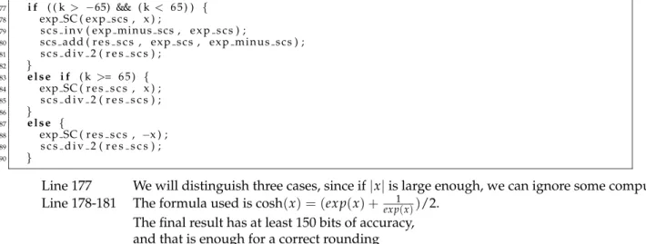
9.1.2 Relation between cosh(x), sinh(x)andex . . . 127
9.1.3 Worst cases for correct rounding . . . 128
9.2 Quick phase . . . 128
9.2.1 Overview of the algorithm . . . 128
9.2.2 Error analysis . . . 129
9.2.3 Details of computer program . . . 131
9.2.4 Rounding . . . 135
9.2.5 Directed rounding . . . 135
9.3 Accurate phase . . . 135
9.4 Analysis of cosh performance . . . 136
Chapter 0
Getting started with crlibm
0.1 What is
crlibm
?
Thecrlibmproject aims at developing a portable, proven, correctly rounded, and efficient mathematical library (libm) for double precision.
correctly rounded Currentlibmimplementation do not always return the floating-point number that is closest to the exact mathematical result. As a consequence, differentlibmimplementation will return different results for the same input, which prevents full portability of floating-point ap-plications. In addition, few libraries support but the round-to-nearest mode of the IEEE754/IEC 60559 standard for floating-point arithmetic (hereafter usually referred to as the IEEE-754 stan-dard).crlibmprovides the four rounding modes: To nearest, to+∞, to−∞and to zero.
portable crlibmis written in C and will be compiled by any compiler fulfilling basic requirements of the ISO/IEC 9899:1999 (hereafter referred to as C99) standard. This is the case ofgccversion 3 and higher which is available on most computer systems. It also requires a floating-point implemen-tation respecting the IEEE-754 standard, which is also available on most modern systems.crlibm has been tested on a large range of systems.
proven Other libraries attempt to provide correctly-rounded result. For theoretical and practical rea-sons, this behaviour is difficult to prove, and in extreme cases termination is not even guaranteed. crlibmintends to provide a comprehensive proof of the theoretical possibility of correct rounding, the algorithms used, and the implementation, assuming C99 and IEEE-754 compliance.
efficient performance and resource usage ofcrlibmshould be comparable to existinglibm implemen-tations, both in average and in the worst case. In contrast, other correctly-rounded libraries have worst case performance and memory consumption several order of magnitude larger than stan-dardlibms.
The ultimate goal of thecrlibmproject is to push towards the standardization of correctly-rounded elementary functions.
0.2 Compilation and installation
See theINSTALLfile in the main directory. This library is developed using the GNU autotools, and can therefore be compiled on most Unix-like systems by./configure; make.
The commandmake checkwill launch the selftest. For more advanced testing you will need to have MPFR installed (seewww.mpfr.org) and to pass the--enable-mpfrflag toconfigure. For other flags, see./configure --help.
0.3 Using
crlibm
functions in your program
Currentlycrlibmfunctions have different names from the standardmath.hfunctions. For example, for the sine function (double sin(double)in the standardmath.h), you have four different functions in crlibmfor the four different rounding modes. These functions are namedsin rn,sin ru,sin rdand sin rzfor round to the nearest, round up, round down and round to zero respectively. These functions are declared in the C header filecrlibm.h.
The crlibm library relies on double-precision IEEE-754 compliant floating-point operations. For some processors and some operating systems (most notably IA32 and IA64 processors under GNU/Linux), the default precision is set to double-extended. On such systems you will need to call thecrlibm init() function before using anycrlibmfunction to ensure such compliance. This has the effect of setting the processor flags to IEEE-754 double-precision with rounding to the nearest mode. This function returns the previous processor status, so that previous mode can be restored using the functioncrlibm exit(). Note that you probably only need one call tocrlibm init()at the beginning of your program, not one call before each call to a mathematical function.
Here’s an example function namedcompare.cusing the cosine function fromcrlibmlibrary. Listing 1: compare.c 1 # include<s t d i o . h> 2 # include<math . h> 3 # include<crlibm . h> 4 5 i n t main (void){
6 double x , res libm , r e s c r l i b m ;
7
8 c r l i b m i n i t ( ) ; /∗ no need h e r e t o s a v e t h e o l d p r o c e s s o r s t a t e r e t u r n e d by c r l i b m i n i t ( ) ∗/
9 p r i n t f ( ” Enter a f l o a t i n g point number : ” ) ; 10 scanf ( ”%l f ” , &x ) ;
11 res libm = cos ( x ) ; 12 r e s c r l i b m = cos rn ( x ) ; 13 p r i n t f ( ”\n x=%.25e \n” , x ) ;
14 p r i n t f ( ”\n cos ( x ) with the system : %.25e \n” , res libm ) ;
15 p r i n t f ( ”\n cos ( x ) with crlibm : %.25e \n” , r e s c r l i b m ) ;
16 return 0 ;
17 }
This example will be compiled withgcc compare.c -lm -lcrlibm -o compare
0.4 Currently available functions
The currently available functions are summarized in the following table, wherexis of typedoubleand every function returns a double-precision number. For trigonometric functions the angles are expressed in radian.
crlibm
C99 to nearest to+∞ to−∞ to zero
cos(x) cos rn(x) cos ru(x) cos rd(x) cos rz(x) sin(x) sin rn(x) sin ru(x) sin rd(x) sin rz(x) tan(x) tan rn(x) tan ru(x) tan rd(x) tan rz(x) cosh(x) cosh rn(x) cosh ru(x) cosh rd(x) cosh rz(x) sinh(x) sinh rn(x) sinh ru(x) sinh rd(x) sinh rz(x) atan(x) atan rn(x) atan ru(x) atan rd(x) atan rz(x) exp(x) exp rn(x) exp ru(x) exp rd(x) exp rz(x)
log(x) log rn(x) log ru(x) log rd(x) log rz(x) log2(x) log2 rn(x) log2 ru(x) log2 rd(x) log2 rz(x) log10(x) log10 rn(x) log10 ru(x) log10 rd(x) log10 rz(x)
0.5 Writing portable floating-point programs
Here are some rules to help you design programs which have to produce exactly the same results on different architectures and different operating systems.
• Try to use the same compiler on all the systems.
• Demand C99 compliance (pass the-C99,-std=c99, or similar flag to the compiler). For Fortran,
demand F90 compliance.
• Callcrlibm init()before you begin floating-point computation. This ensures that the compu-tations will all be done in IEEE-754 double-precision with round to nearest mode, which is the largest precision well supported by most systems. On IA32 processors, problems may still occur for extremely large or extremely small values.
• Do not hesitate to rely heavily on parentheses (the compiler should respect them according to
the standards, although of course some won’t). Many times, wondering where the parentheses should go in an expression likea+b+c+dwill even help you improve the accuracy of your code.
Chapter 1
Introduction: Goals and methods
1.1 Correct rounding and elementary functions
The need for accurate elementary functions is important in many critical programs. Methods for com-puting these functions include table-based methods[17, 34], polynomial approximations and mixed methods[9]. See the books by Muller[31] or Markstein[28] for recent surveys on the subject.
The IEEE-754 standard for floating-point arithmetic[6] defines the usual floating-point formats (sin-gle and double precision). It also specifies the behavior of the four basic operators (+,−,×,÷) and
the square root in four rounding modes (to the nearest, towards+∞, towards−∞and towards 0). Its adoption and widespread use have increased the numerical quality of, and confidence in floating-point code. In particular, it has improvedportabilityof such code and allowed construction of proofson its numerical behavior. Directed rounding modes (towards+∞,−∞and 0) also enabled efficientinterval
arithmetic[29, 21].
However, the IEEE-754 standard specifies nothing about elementary functions, which limits these advances to code excluding such functions. Currently, several options exist: on one hand, one can use today’s mathematical libraries that are efficient but without any warranty on the correctness of the results. To be fair, most modern libraries areaccurate-faithful: trying to round to nearest, they return a number that is one of the two FP numbers surrounding the exact mathematical result, and indeed return the correctly rounded result most of the time. This behaviour is sometimes described using phrases like
99% correct roundingor0.501 ulp accuracy.
When stricter guarantees are needed, some multiple-precision packages like MPFR [30] offer correct rounding in all rounding modes, but are several orders of magnitude slower than the usual mathe-matical libraries for the same precision. Finally, there are are currently three attempts to develop a correctly-rounded libm. The first was IBM’s libultim[27] which is both portable and fast, if bulky, but lacks directed rounding modes needed for interval arithmetic. The second was Ar´enaire’scrlibm, which was first distributed in 2003. The third is Sun correctly-rounded mathematical library called libmcr, whose first beta version appeared in 2004. These libraries are reviewed in 1.4.
The goal of thecrlibmproject is to build on a combination of several recent theoretical and algorith-mic advances to design a proven correctly rounded mathematical library, with an overhead in terms of performance and resources acceptable enough to replace existing libraries transparently.
More generally, the crlibmproject serves as an open-source framework for research on software elementary functions. As a side effect, it may be used as a tutorial on elementary function development.
1.2 A methodology for efficient correctly-rounded functions
1.2.1 The Table Maker’s Dilemma
With a few exceptions, the image ˆy of a floating-point number x by a transcendental function f is a transcendental number, and can therefore not be represented exactly in standard numeration systems. The only hope is to compute the floating-point number that is closest to (resp. immediately above or
immediately below) the mathematical value, which we call the resultcorrectly rounded to the nearest (resp. towards+∞or towards−∞).
It is only possible to compute an approximationyto the real number ˆywith precisionε. This ensures
that the real value ˆy belongs to the interval[y(1−ε),y(1+ε)]. Sometimes however, this information
is not enough to decide correct rounding. For example, if[y(1−ε),y(1+ε)] contains the middle of
two consecutive floating-point numbers, it is impossible to decide which of these two numbers is the correctly rounded to the nearest of ˆy. This is known as the Table Maker’s Dilemma (TMD). For example, if we consider a numeration system in radix 2 withn-bit mantissa floating point number andmthe number of significant bit inysuch thatε≤2m, then the TMD occurs:
• for rounding toward+∞,−∞, 0, when the result is of the form:
m bits z }| { 1.|xxx{z...xx} n bits 111111...11xxx... or: m bits z }| { 1.|xxx{z...xx} n bits 000000...00xxx...
• for rounding to nearest, when the result is of the form:
m bits z }| { 1.|xxx{z...xx} n bits 011111...11xxx... or : m bits z }| { 1.|xxx{z...xx} n bits 100000...00xxx...
1.2.2 The onion peeling strategy
A method described by Ziv [36] is to increase the precisionεof the approximation until the correctly
rounded value can be decided. Given a function f and an argument x, the value of f(x)is first
eval-uated using a quick approximation of precisionε1. Knowing ε1, it is possible to decide if rounding is
possible, or if more precision is required, in which case the computation is restarted using a slower approximation of precisionε2greater thanε1, and so on. This approach makes sense even in terms of
average performance, as the slower steps are rarely taken.
However there was until recently no practical bound on the termination time of such an algorithm. This iteration has been proven to terminate, but the actual maximal precision required in the worst case is unknown. This might prevent using this method in critical application.
1.3 The Correctly Rounded Mathematical Library
Our own library, calledcrlibmforcorrectly rounded mathematical library, is based on the work of Lef`evre and Muller [24, 25] who computed the worst-caseεrequired for correctly rounding several functions
in double-precision over selected intervals in the four IEEE-754 rounding modes. For example, they proved that 157 bits are enough to ensure correct rounding of the exponential function on all of its domain for the four IEEE-754 rounding modes.
1.3.1 Two steps are enough
Thanks to such results, we are able to guarantee correct rounding in two iterations only, which we may then optimize separately. The first of these iterations is relatively fast and provides between 60 and 80 bits of accuracy (depending on the function), which is sufficient in most cases. It will be referred
throughout this document as the quick phase of the algorithm. The second phase, referred to as the accurate phase, is dedicated to challenging cases. It is slower but has a reasonably bounded execution time, tightly targeted at Lef`evre’s worst cases.
Having a proven worst-case execution time lifts the last obstacle to a generalization of correctly rounded transcendentals. Besides, having only two steps allows us to publish, along with each function, a proof of its correctly rounding behavior.
1.3.2 Portable IEEE-754 FP for a fast first step
The computation of a tight bound on the approximation error of the first step (ε1) is crucial for the
efficiency of the onion peeling strategy: overestimatingε1means going more often than needed through
the second step, as will be detailed below in 1.3.5. As we want the proof to be portable as well as the code, our first steps are written in strict IEEE-754 arithmetic. On some systems, this means preventing the compiler/processor combination to use advanced floating-point features such as fused multiply-and-add or extended double precision. It also means that the performance of our portable library will be lower than optimized libraries using these features (see [12] for recent research on processor-specific correct-rounding).
To ease these proofs, our first steps make wide use of classical, well proven results like Sterbenz’ lemma or other floating-point theorems. When a result is needed in a precision higher than double precision (as is the case ofy1, the result of the first step), it is represented as as the sum of two floating-point numbers, also called adouble-doublenumber. There are well-known algorithms for computing on double-doubles, and they are presented in the next chapter. An advantage of properly encapsulating double-double arithmetic is that we can actually exploit fused multiply-and-add operators in a trans-parent manner (this experimental feature is currently available for the Itanium and PowerPC platforms, when using thegcccompiler).
At the end of the quick phase, a sequence of simple tests ony1knowingε1allows to decide whether
to go for the second step. The sequence corresponding to each rounding mode is shared by most func-tions and is also carefully proven in the next chapter.
1.3.3 Software Carry-Save for an accurate second step
For the second step, we designed an ad-hoc multiple-precision library called Software Carry-Save li-brary(scslib)which is lighter and faster than other available libraries for this specific application [14, 10]. This choice is motivated by considerations of code size and performance, but also by the need to be in-dependent of other libraries: Again, we need a library on which we may rely at the proof level. This library is included incrlibm, but also distributed separately [3]. This library is described in more details in 2.7.
1.3.4 Proving the correct rounding property
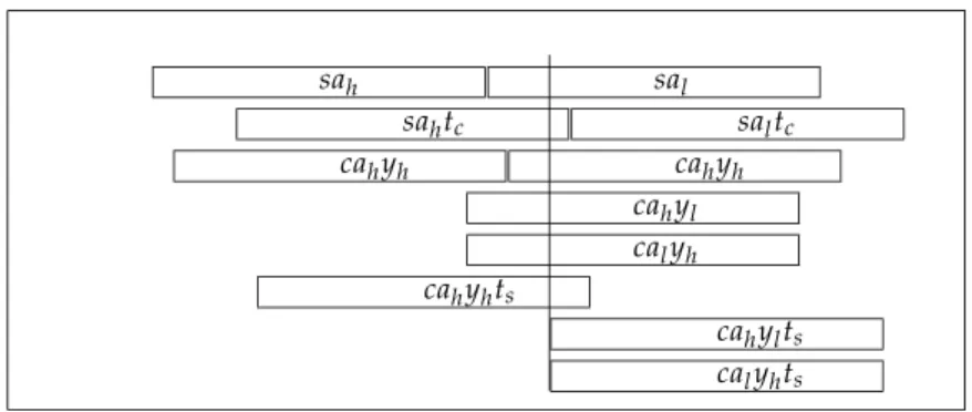
Throughout this document, what we call “proving” a function mostly means proving a tight bound on the total relative error of our evaluation scheme. The actual proof of the correct rounding property is then dependent on the availability of an actual worst-case accuracy for correctly rounding this function, as computed by Lef`evre and Muller. Three cases may happen:
• The worst case have been computed over the whole domain of the function. In this case the
correct rounding property for this function is fully proven. As ofcrlibm0.8, this is the case of the exponential and natural logarithm functions, and for the hyperbolic sine and cosine. The inverse trigonometric functions should follow soon.
• The worst cases have been computed only over a subdomain of the function. Then the correct
rounding property is proven on this subdomain. Outside of this domaincrlibmoffers “astronom-ical confidence” that the function is correctly rounded: to the best of current knowledge [18, 12], the probability of the existence of a misrounded value in the function’s domain is lower than 2−40.
As ofcrlibm0.8, this is the case of the trigonometric functions and the arctangent. The actual do-main on which the proof is complete is mentionned in the respective chapter of this document, and summed up below in 1.3.6.
• The search for worst cases hasn’t begun yet.
We acknowledge that the notion of astronomical confidence breaks the objective of guaranteed cor-rect rounding, and we sidestep this problem by publishing along with the library (in this document) the domain of full confidence, which will only expand as time goes. Such behaviour has been proposed as a standard in [15]. The main advantage of this approach is that it ensures bounded and consistent worst-case execution time (within a factor 100 of that of the best available faithfullibms), which we believe is crucial to the generalization of correctly rounded functions.
The alternative to our approach would be to implement a multi-layer onion-peeling strategy, as do GNU MPFR and Sun’slibmcr. There are however many drawbacks to this approach, too:
• One may argue that, due to the finite nature of computers, it only pushes the bounds of astronomy
a little bit further.
• The multilayer approach is only proven to terminate on elementary functions: the termination
proof needs a theorem stating for example that the image of a rational by the function (with some well-known exceptions) will not be a rational. For other library functions like special functions, we have no such theorem. For these functions, we prefer take the risk of a misrounded value than the risk of an infinite loop.
• Similarly, the multilayer approach has potentially unbounded execution time and memory
con-sumption which make it unsuitable for real-time or safety-critical applications, whereas crlibm will only be unsuitable if the safety depends on correct rounding, which is much less likely.
• Multilayer code is probably much more complex and error prone. One important problem is
that it contains code that, according all probabilities, will never be run. Therefore, testing this code can not be done on the final production executable, but on a different executable in which previous layers have been disabled. This introduces the possibility of undetected bugs in the final production executable.
In the future, we will add, to thosecrlibmfunctions for which the required worst-case accuracy is unknown, a misround detection test at the end of the second step. This test will either print out on standard error a lengthy warning inviting to report this case, or launch MPFR computation, depending on a compilation switch.
1.3.5 Error analysis and the accuracy/performance tradeoff
As there are two steps on the evaluation, the proof also usually consists of two parts. The code of the second, accurate step is usually very simple and straightforward:
• Performance is not that much of an issue, since this step is rarely taken. • All the special cases have already been filtered by the first step.
• Thescsliblibrary provides an overkill of precision.
Therefore, the error analysis of the second step, which ultimately proves the correct rounding prop-erty, is not very difficult.
For the first step, however, things are more complicated:
• We have to handle special cases (infinities, NaNs, signed zeroes, over- and underflows). • Performance is a primary concern, sometimes leading to “dirty tricks” obfuscating the code. • We have to compute atighterror bound, as explained below.
Why do we need a tight error bound? Because the decision to launch the second step is taken by a
rounding testdepending on
• the approximationyh+ylcomputed in the first step, and
The various rounding tests are detailed and proven in 2.6. The important notion here is thatthe probability of launching the second, slower step will be proportional to the error boundε1computed for the first step.
This defines the main performance tradeoff one has to manage when designing a correctly-rounded function: The average evaluation time will be
Tavg=T1+p2T2 (1.1)
whereT1andT2are the execution time of the first and second phase respectively (withT2 ≈100T1in
crlibm), andp2is the probability of launching the second phase (typically we aim atp2 =1/1000 so
that the average cost of the second step is less than 10% of the total.
Asp2is almost proportional toε1, to minimise the average time, we have to
• balanceT1andp2: this is a performance/precision tradeoff (the faster the first step, the less
accu-rate)
• and compute a tight bound on the overall errorε1.
Computing this tight bound is the most time-consuming part in the design of a correctly-rounded elementary function. The proof of the correct rounding property only needs a proven bound, but a loose bound will mean a largerp2than strictly required, which directly impacts average performance. Comparep2=1/1000 andp2 =1/500 forT2 =100T1, for instance. As a consequence, when there are
multiple computation paths in the algorithm, it makes sense to precompute different values ofε1on
these different paths (see for instance the arctangent and the logarithm).
Apart from these considerations, computing the errors is mostly textbook science. Care must be taken that onlyabsoluteerror terms (notedδ) can be added, although some error terms (like the rounding
error of an IEEE operation) are best expressed asrelative(notedε). Remark also that the error needed for
the theorems in 2.6 is arelativeerror. Managing the relative and absolute error terms is very dependent on the function, and usually involves keeping upper and lower bounds on the values manipulated along with the error terms.
Error terms to consider are the following:
• approximation errors (minimax or Taylor), • rounding error, which fall into two categories:
– roundoff errors in values tabulated as doubles or double-doubles (with the exception of roundoff errors on the coefficient of a polynomial, which are counted in the appproxima-tion error),
– roundoff errors in IEEE-compliant operations.
1.3.6 Current state of
crlibm
The crlibm library currently offers accurate parts for the exponential, logarithm in radix 2, 10 and
e, sine, cosine, tangent, arctangent, plus trigonometric argument reduction. The quick part and its proof have been written for the exponential, natural logarithm, sine, cosine tangent, arctangent, and the hyperbolic sine and cosine thus far.
The correct rounding property is fully proven (the worst-case required accuracy has been deter-mined) on the following intervals (Fdenotes the set of IEEE-754 doubles, and indicate a fully proven function):
Function interval exp F log F log 2 F log 10 F cosh F sinh F sin [−π/2,π/2] cos [−2, 2] tan [−2−3, 2−3]
arctan [−tan(2−3), tan(2−3)]
1.4 An overview of other available mathematical libraries
Many high-quality mathematical libraries are freely available and have been a source of inspiration for this work.
Most mathematical libraries do not offer correct rounding. They can be classified as
• portable libraries assuming IEEE-754 arithmetic, likefdlibm, written by Sun[4]; • Processor-specific libraries, by Intel[20, 2] and HP[28, 26] among other.
Operating systems often include several mathematical libraries, some of which are derivatives of one of the previous.
To our knowledge, three libraries currently offer correct rounding:
• Thelibultimlibrary, also called MathLib, is developed at IBM by Ziv and others [27]. It provides
correct rounding, under the assumption that 800 bits are enough in all case. This approach suffers two weaknesses. The first is the absence of proof that 800 bits are enough: all there is is a very high probability. The second is that, as we will see in the sequel, for challenging cases, 800 bits are much of an overkill, which can increase the execution time up to 20,000 times a normal execution. This will prevent such a library from being used in real-time applications. Besides, to prevent this worst case from degrading average performance, there is usually some intermediate levels of precision in MathLib’s elementary functions, which makes the code larger, more complex, and more difficult to prove (and indeed this library is scarcely documented).
In addition this library provides correct rounding only to nearest. This is the most used round-ing mode, but it might not be the most important as far as correct roundround-ing is concerned: correct rounding provides a precision improvement over current mathematical libraries of only a fraction of a unit in the last place(ulp). Conversely, the three other rounding modes are needed to guaran-tee intervals in interval arithmetic. Without correct rounding in these directed rounding modes, interval arithmetic looses up to oneulpof precision in each computation.
• MPFRis a multiprecision package safer thanlibultilmas it uses arbitrary multiprecision. It
pro-vides most of elementary functions for the four rounding modes defined by the IEEE-754 stan-dard. However this library is not optimized for double precision arithmetic. In addition, as its exponent range is much wider than that of IEEE-754, the subtleties of subnormal numbers are difficult to handle properly using such a multiprecision package.
• The libmcr library, by K.C. Ng, Neil Toda and others at Sun Microsystems, had its first beta version published in december 2004. Its purpose is to be a reference implementation for correctly rounded functions in double precision. It has very clean code, offers arbitrary multiple precision unlikelibultim, at the expense of slow performance (due to, for example dynamic allocation of memory). It offers the directed rounding modes, and rounds in the mode read from the processor status flag.
1.5 Various policies in
crlibm
1.5.1 Naming the functions
Currentcrlibmdoesn’t by default replace your existinglibm: the functions incrlibmhave the C99 name, suffixed with rn, ru, rd, and rzfor rounding to the nearest, up, down and to zero respectively. They require the processor to be in round to nearest mode. Starting with version 0.9 we should provide a compile-time flag which will overload the defaultlibmfunctions with the crlibm ones with rounding to nearest.
It is interesting to compare this to the behaviour of Sun’s library: First, Sun’slibmcrprovides only one function for each C99 function instead of four incrlibm, and rounds according to the processor’s current mode. This is probably closer to the expected long-term behaviour of a correctly-rounded math-ematical library, but with current processors it may have a tremendous impact on performance. Besides, the notion of “current processor rounding mode” is no longer relevant on recent processors like the Ita-nium family, which have up to four different modes at the same time. A second feature oflibmcris that it overloads by default the systemlibm.
The policy implemented in currentcrlibmintends to provide best performance to the two classes of users who will be requiring correct rounding: Those who want predictible, portable behaviour of floating-point code, and those who implement interval arithmetic. Of course, we appreciate any feed-back on this subject.
1.5.2 Policy concerning IEEE-754 flags
Currently, thecrlibmfunctions try to raise the Overflow and Underflow flags properly. Raising the other flags (especially the Inexact flag) is possible but considered too costly for the expected use, and will usually not be implemented. We also appreciate feedback on this subject.
1.5.3 Policy concerning conflicts between correct rounding and expected
mathe-matical properties
As remarked in [15], it may happen that the requirement of correct rounding conflicts with a basic math-ematical property of the function, such as its domain and range. A typical example is the arctangent of a very large number which, rounded up, will be a number larger thanπ/2 (fortunately,◦(π/2)<π/2).
The policy that will be implemented incrlibmwill be
• to give priority to the mathematical property in round to nearest mode (so as not to hurt the
innocent user who may expect such a property to be respected), and
• to give priority to correct rounding in the directed rounding modes, in order to provide trustful
bounds to interval arithmetic. Again, this policy is open to discussion.
1.6 Organization of the source code
For each function, the file containing the source code for the accurate phase is named after the function with the accuratesuffix (for instanceexp accurate.c,log accurate.c), and the quick phase, when available, is named with the fastsuffix (for instanceexp fast.c). The names of auxiliary files.cor .hfiles relative to a function are also prefixed with the name of the function.
The accurate phase relies onscslib, thesoftware carry-savemultiple-precision library written for this purpose. This library is contained in a subdirectory calledscs lib.
The common C routines that are detailed in Chapter 2 of this document are defined incrlibm private.c andcrlibm private.h.
Many of the constants used in the C code have been computed thanks to Maple procedures which are contained in themaplesubdirectory. Some of these procedures are explained in Chapter 2. For some functions, a Maple procedure mimicking the C code, and used for debugging or optimization purpose, is also available.
The code also includes programs to test thecrlibmfunctions against MPFR andlibultim, in terms of correctness and performance. They are located in thetestsdirectory.
Chapter 2
Common notations, theorems and
procedures
2.1 Notations
The following notations will be used throughout this document:
• +,−and×denote the usual mathematical operations.
• ⊕,ªand⊗denote the corresponding floating-point operations in IEEE-754 double precision, in
the IEEE-754round to nearestmode.
• ◦(x),4(x)and5(x)denote the value ofxrounded to the nearest, resp. rounded up and down.
• ε(usually with some index) denotes a relative error,δdenotes an absolute error. Upper bounds
on the absolute value of these errors will be denotedεandδ.
• ε−k– with a negative index – represents an erroresuch that|e| ≤2−k.
• For a floating-point number x, the value of the least significant bit of its mantissa is classically
denoted ulp(x).
2.2 Common C procedures for double-precision numbers
2.2.1 Sterbenz Lemma
Theorem 1 (Sterbenz Lemma [33, 19]). If x and y are floating-point numbers, and if y/2 ≤ x ≤ 2y then
xªy is computed exactly, without any rounding error.
2.2.2 Double-precision numbers in memory
A double precision floating-point number uses 64 bits. The unit of memory in most current architectures is a 32-bit word. The order in which the two 32 bits words of a double are stored in memory depends on the architecture. An architecture is saidLittle Endianif the lower part of the number is stored in memory at the smallest address; It is the case of the x86 processors. Conversely, an architecture with the high part of the number stored in memory at the smallest address is saidBig Endian; It is the case of the PowerPC processors.
Incrlibm, we extract the higher and lower parts of a double by using an union in memory: the type db number. The following code extracts the upper and lower part from a double precision numberx.
Listing 2.1: Extract upper and lower part of a double precision numberx
1 /∗ HI and LO a r e d e f i n e d a u t o m a t i c a l l y by a u t o c o n f / automake . ∗/
2
4 i n t x hi , x l o ; 5 xx . d = x ; 6 x h i = xx . i [ HI ] 7 x l o = xx . i [LO]
2.2.3 Conversion from floating-point to integer
Theorem 2 (Conversion floating-point to integer). The following algorithm, taken from [5], converts a double-precision floating-point number d into a 32-bit integer i with rounding to nearest mode.
It works for all the doubles whose nearest integer fits on a 32-bit machine signed integer.
Listing 2.2: Conversion from FP to int
1 # d e f i n e DOUBLE2INT( i , d ) \
2 {double t =( d +6755399441055744.0) ; i =LO( t ) ;}
This algorithm adds the constant 252+251to the floating-point number to put the integer part ofx,
in the lower part of the floating-point number. We use 252+251 and not 252, because the value 251 is
used to contain possible carry propagations with negative numbers.
2.2.4 Conversion from floating-point to 64-bit integer
Theorem 3 (Conversion floating-point to a long long integer). The following algorithm, is derived from the previous.
It works for any double whose nearest integer is smaller than251−1.
Listing 2.3: Conversion from FP to long long int
1 # d e f i n e DOUBLE2LONGINT( i , d ) \ 2 { \ 3 db number t ; \ 4 t . d = ( d +6755399441055744.0) ; \ 5 i f ( d >= 0) /∗ s i g n e x t e n d ∗/ \ 6 i = t . l & 0x0007FFFFFFFFFFFFLL ; \ 7 e l s e \ 8 i = ( t . l & 0x0007FFFFFFFFFFFFLL ) | (0 xFFF8000000000000LL ) ; \ 9 }
2.2.5 Methods to raise IEEE-754 flags
The IEEE standard imposes, in certain cases, to raise flags and/or exceptions for the 4 operators (+,×, ÷,√). Therefore, it is legitimate to require the same for elementary functions.
In ANSI-C99, the following instructions raise exceptions and flags:
• underflow : the multiplication ±smallest×smallest wheresmallest correspond to the smallest
subnormal number,
• overflow: the multiplication±largest×largestwherelargestcorrespond to the largest
normal-ized number,
• division by zero: the division±1.0/0.0,
• inexact : the addition (x+smallest)−smallestwhere x is the result and smallestthe smallest
subnormal number,
2.3 Common C procedures for double-double arithmetic
Hardware operators are usualy limited to double precision. To perform operations with more precision, then software solutions need to be used. One among them is to represent a floating point number as the sum of two non-overlapping floating-point numbers (ordouble-doublenumbers).
The algorithms are given as plain C functions, but it may be preferable, for performance issue, to im-plement them as macros, as inlibultim. The code offers both versions, selected by theDEKKER AS FUNCTIONS constant which is set by default to 1 (functions).
A more recent proof is available in [23].
2.3.1 Exact sum algorithm Add12
This algorithm is also known as the Fast2Sum algorithm in the litterature.
Theorem 4 (Exact sum [22, 7]). Let a and b be floating-point numbers, then the following method computes two floating-point numbers s and r, such that s+r=a+b exactly, and s is the floating-point number which is
closest to a+b.
Listing 2.4: Add12Cond
1 void Add12Cond (double ∗s , double ∗r , a , b )
2 { 3 double z ; 4 s = a + b ; 5 i f (ABS( a ) > ABS( b ) ){ 6 z = s − a ; 7 r = b − z ; 8 }e l s e { 9 z = s − b ; 10 r = a − z ; 11 } 12 }
Here ABS is a macro that returns the absolute value of a floating-point number. This algorithm requires4 floating-point additions and2floating point tests (some of which are hidden in the ABS macro).
Note that if it is more efficient on a given architecture, the test can be replaced with a test on the exponents of a and b.
If we are able to prove that the exponent of ais always greater than that ofb, then the previous algorithm to perform an exact addition of 2 floating-point numbers becomes :
Listing 2.5: Add12
1 void Add12 (double ∗s , double ∗r , a , b )
2 { 3 double z ; 4 s = a + b ; 5 z = s − a ; 6 r = b − z ; 7 }
The cost of this algorithm is 3 floating-point additions.
2.3.2 Exact product algorithm Mul12
This algorithm is sometimes also known as the Dekker algorithm [16]. It was proven by Dekker but the proof predates the IEEE-754 standard and is difficult to read. An easier proof is available in [19] (see Th. 14).
Theorem 5 (Restricted exact product). Let a and b be two double-precision floating-point numbers, with 53 bits of mantissa. Let c=2d532e+1. Assuming that a<2970and b<2970, the following procedure computes the
two floating-point numbers rh and rl such that rh+rl =a+b with rh=a⊗b:
Listing 2.6: Mul12
2 const double c = 1 3 4 2 1 7 7 2 9 . ; /∗ 1+2ˆ27 ∗/ 3 double up , u1 , u2 , vp , v1 , v2 ; 4 5 up = u∗c ; vp = v∗c ; 6 u1 = ( u−up )+up ; v1 = ( v−vp )+vp ; 7 u2 = u−u1 ; v2 = v−v1 ; 8 9 ∗rh = u∗v ; 10 ∗r l = ( ( ( u1∗v1−∗rh ) +( u1∗v2 ) ) +( u2∗v1 ) ) +( u2∗v2 ) ; 11 }
The cost of this algorithm is 10 floating-point additions and 7 floating-point multiplications. The condition a < 2970 and b < 2970 prevents overflows when multiplying by c. If it cannot be
proved statically, then we have to first testaandb, and prescale them so that the condition is true. Theorem 6 (Exact product). Let a and b be two double-precision floating-point numbers, with 53 bits of man-tissa. Let c=2d532e+1. The following procedure computes the two floating-point numbers rh and rl such that rh+rl=a+b with rh=a⊗b:
Listing 2.7: Mul12Cond
1 void Mul12Cond (double ∗rh , double ∗r l , double a , double b ){
2 const double two 970 = 0.997920154767359905828186356518419283 e292 ; 3 const double two em53 = 0.11102230246251565404236316680908203125 e−15; 4 const double two e53 = 9007199254740992.;
5 double u , v ; 6
7 i f ( a>two 970 ) u = a∗two em53 ;
8 e l s e u = a ;
9 i f ( b>two 970 ) v = b∗two em53 ;
10 e l s e v = b ; 11
12 Mul12 ( rh , r l , u , v ) ; 13
14 i f ( a>two 970 ) {∗rh ∗= two e53 ; ∗r l ∗= two e53 ;}
15 i f ( b>two 970 ) {∗rh ∗= two e53 ; ∗r l ∗= two e53 ;}
16 }
The cost in the worst case is then 4 tests over integers, 10 point additions and 13 floating-point multiplications.
Finally, note that a fused multiply-and-add provides the Mul12 and Mul12Cond in only two instruc-tions [8]. Here is the example code for the Itanium processor.
Listing 2.8: Mul12 on the Itanium
1 # define Mul12Cond ( rh , r l , u , v ) \ 2 { \ 3 ∗rh = u∗v ; \ 4 /∗ The f o l l o w i n g means : ∗r l = FMS( u∗v−∗rh ) ∗/ \ 5 asm v o l a t i l e ( ”fms %0 = %1, %2, %3\n ; ;\n” \ 6 : ”= f ” (∗r l ) \ 7 : ” f ” ( u ) , ” f ” ( v ) , ” f ” (∗rh ) \ 8 ) ; \ 9 }
10 # define Mul12 Mul12Cond
Thecrlibmdistribution attempts to use the FMA for systems on which it is availables (currently Itanium and PowerPC).
2.3.3 Double-double addition Add22
This algorithm, also due to Dekker [16], computes the sum of two double numbers as a double-double, with a relative error smaller than 2−103(there is a proof in [16], a more recent one can be found
in in [23]).
Listing 2.9: Add22Cond
1 void Add22Cond (double ∗zh , double ∗zl , double xh , double xl , double yh , double yl )
2 {
4
5 r = xh+yh ;
6 s = (ABS( xh ) > ABS( yh ) ) ? ( xh−r+yh+yl+ x l ) : ( yh−r+xh+ x l +yl ) ;
7 ∗zh = r+s ;
8 ∗z l = r − (∗zh ) + s ;
9 }
Here ABS is a macro that returns the absolute value of a floating-point number. Again, if this test can be resolved at compile-time, we get the fasterAdd22procedure:
Listing 2.10: Add22
1 void Add22 (double ∗zh , double ∗zl , double xh , double xl , double yh , double yl )
2 { 3 double r , s ; 4 5 r = xh+yh ; 6 s = xh−r+yh+yl+ x l ; 7 ∗zh = r+s ; 8 ∗z l = r − (∗zh ) + s ; 9 }
2.3.4 Double-double multiplication Mul22
This algorithm, also due to Dekker [16], computes the product of two double-double numbers as a double-double, with a relative error smaller than 2−102, under the conditionx
h < 2970 andyh < 2970
(there is a proof in [16], a more recent one can be found in in [23]). Listing 2.11: Mul22
1 void Mul22 (double ∗zh , double ∗zl , double xh , double xl , double yh , double yl )
2 {
3 double mh, ml ;
4
5 const double c = 1 3 4 2 1 7 7 2 9 . ; /∗ 0x41A00000 , 0 x02000000 ∗/
6 double up , u1 , u2 , vp , v1 , v2 ; 7 8 up = xh∗c ; vp = yh∗c ; 9 u1 = ( xh−up ) +up ; v1 = ( yh−vp ) +vp ; 10 u2 = xh−u1 ; v2 = yh−v1 ; 11 12 mh = xh∗yh ;
13 ml = ( ( ( u1∗v1−mh) +(u1∗v2 ) ) +(u2∗v1 ) ) +(u2∗v2 ) ;
14
15 ml += xh∗yl + x l∗yh ;
16 ∗zh = mh+ml ;
17 ∗z l = mh− (∗zh ) + ml ;
18 }
Note that the bulk of this algorithm is a Mul12(mh,ml,xh,yh). Of course there is a conditional version of this procedure but we have not needed it so far.
Our algorithms will sometimes need to multiply a double by a double-double. In this case we use Mul22with one of the arguments set to zero, which only performs one useless multiplication by zero and one useless addition: a specific procedure is not needed.
2.3.5 Multiplication of a double-double by an integer
Use Cody and Waite algorithm. See for instance the log and the trigonometric argument reduction (chapter 3, p. 41).
2.4 Common C procedures for triple-double arithmetic
2.4.1 The addition operator Add33
Algorithm 1 (Add33).
In:two triple-double numbers, ah+am+alet bh+bm+bl
Out:a triple-double number rh+rm+rl
Preconditions on the arguments:
|bh| ≤ 34· |ah| |am| ≤ 2−αo· |ah| |al| ≤ 2−αu· |am| |bm| ≤ 2−βo· |bh| |bl| ≤ 2−βu· |bm| αo ≥ 4 αu ≥ 1 βo ≥ 4 βu ≥ 1 Algorithm: (rh,t1)←Add12(ah,bh) (t2,t3)←Add12(am,bm) (t7,t4)←Add12(t1,t2) t6←al⊕bl t5←t3⊕t4 t8←t5⊕t6 (rm,rl)←Add12(t7,t8)
Theorem 7 (Relative error of algorithm 1 Add33).
Let be ah+am+al and bh+bm+bl the triple-double arguments of algorithm 1Add33 verifying the given preconditions.
So the following egality will hold for the returned values rh, rmet rl
rh+rm+rl= ((ah+am+al) + (bh+bm+bl))·(1+ε)
whereεis bounded by:
|ε| ≤2−min(αo+αu,βo+βu)−47+2−min(αo,βo)−98
The returned values rmand rlwill not overlap at all and the overlap of rhand rmwill be bounded by the following expression:
|rm| ≤2−min(αo,βo)+5· |r
h|
2.4.2 The addition operator Add233
Algorithm 2 (Add233).
In:a double-double number ah+aland a triple-double number bh+bm+bl
Out:a triple-double number rh+rm+rl
Preconditions on the arguments:
|bh| ≤ 2−2· |ah| |al| ≤ 2−53· |ah|
|bm| ≤ 2−βo· |bh|
|bl| ≤ 2−βu· |bm|
(rh,t1)←Add12(ah,bh) (t2,t3)←Add12(al,bm) (t4,t5)←Add12(t1,t2) t6←t3⊕bl t7←t6⊕t5 (rm,rl)←Add12(t4,t7)
Theorem 8 (Relative error of algorithm 2 Add233).
Let be ah+aland bh+bm+blthe values taken in argument of algorithm 2Add233. Let the preconditions hold for this values.
So the following holds for the values returned by the algorithm rh, rmet rl
rh+rm+rl= ((ah+am+al) + (bh+bm+bl))·(1+ε) whereεis bounded by
|ε| ≤2−βo−βu−52+2−βo−104+2−153
The values rmand rlwill not overlap at all and the overlap of rhand rmwill be bounded by:
|rm| ≤2−γ· |rh| with
γ≥min(45,βo−4,βo+βu−2)
2.4.3 The multiplication procedure Mul23
Algorithm 3 (Mul23).
In:two double-double numbers ah+aland bh+bl
Out:a triple-double number rh+rm+rl
Preconditions on the arguments:
|al| ≤ 2−53· |ah| |bl| ≤ 2−53· |bh| Algorithm: (rh,t1)←Mul12(ah,bh) (t2,t3)←Mul12(ah,bl) (t4,t5)←Mul12(al,bh) t6←al⊗bl (t7,t8)←Add22(t2,t3,t4,t5) (t9,t10)←Add12(t1,t6) (rm,rl)←Add22(t7,t8,t9,t10)
Theorem 9 (Relative error of algorithm 3 Mul23).
Let be ah+aland bh+blthe values taken by arguments of algorithm 3Mul23
So the following holds for the values returned rh, rmand rl:
rh+rm+rl= ((ah+al)·(bh+bl))·(1+ε)
whereεis bounded as follows:
|ε| ≤2−149
The values returned rmand rlwill not overlap at all and the overlap of rhet rmwill be bounded as follows:
2.4.4 The multiplication procedure Mul233
Algorithm 4 (Mul233).
In:a double-double number ah+aland a triple-double number bh+bm+bl
Out:a triple-double number rh+rm+rl
Preconditions on the arguments:
|al| ≤ 2−53· |ah| |bm| ≤ 2−βo· |bh| |bl| ≤ 2−βu· |bm| with βo ≥ 2 βu ≥ 1 Algorithm: (rh,t1)←Mul12(ah,bh) (t2,t3)←Mul12(ah,bm) (t4,t5)←Mul12(ah,bl) (t6,t7)←Mul12(al,bh) (t8,t9)←Mul12(al,bm) t10 ←al⊗bl (t11,t12)←Add22(t2,t3,t4,t5) (t13,t14)←Add22(t6,t7,t8,t9) (t15,t16)←Add22(t11,t12,t13,t14) (t17,t18)←Add12(t1,t10) (rm,rl)←Add22(t17,t18,t15,t16)
Theorem 10 (Relative error of algorithm 4 Mul233).
Let be ah+aland bh+bm+blthe values in argument of algorithm 4Mul233 such that the given preconditions
hold.
So the following will hold for the values rh, rmand rlreturned
rh+rm+rl= ((ah+al)·(bh+bm+bl))·(1+ε)
whereεis bounded as follows:
|ε| ≤ 2−
99−βo+2−99−βo−βu+2−152
1−2−53−2−βo+1−2−βo−βu+1 ≤2−
97−βo+2−97−βo−βu+2−150
The values rmand rlwill not overlap at all and the following bound will be verified for the overlap of rhand rm:
|rm| ≤2−γ· |rh| where
γ≥min(48,βo−4,βo+βu−4)
2.4.5 Final rounding to the nearest even
Algorithm 5 (Final rounding to the nearest (even)). In:a triple-double number xh+xm+xl
Out:a double precision number x0returned by the algorithm
Preconditions on the arguments:
• xm=◦(xm+xl) • xh6=0, xm6=0et xl6=0 • ◦(xh+xm)6∈©xh−,xh,xh+ª⇒ |(xh+xm)− ◦(xh+xm)| 6=12·ulp(◦(xh+xm)) Algorithm: t1←x−h t2←xhªt1 t3←t2⊗12 t4←x+h t5←t4ªxh t6←t5⊗12 if(xm6=−t3)and(xm6=t6)then return (xh⊕xm) else if(xm⊗xl>0.0)then if(xh⊗xl>0.0)then return x+ h else return x− h end if else return xh end if end if
Theorem 11 (Correctness of the final rounding procedure 5).
Let beAthe algorithm 5 said “ Final rounding to the nearest (even)”. Let be xh+xm+xltriple-double number for which the preconditions of algorithmAhold. Let us notate x0 the double precision number returned by the procedure.
So
x0 =◦(xh+xm+xl)
i.e.Ais a correct rounding procedure for round-to-nearest-ties-to-even mode.
2.4.6 Final rounding for the directed modes
Theorem 12 (Directed final rounding of a triple-double number).
Let be xh+xm+xl∈F+F+Fa non-overlapping triple-double number. Let be¦a directed rounding mode.
Let beAthe following instruction sequence:
(t1,t2)←Add12(xh,xm)
t3←t2⊕xl
return ¦(t1+t3)
SoAis a correct rounding procedure for the rounding mode¦.
2.5 Horner polynomial approximations
Most function evaluation schemes include some kind of polynomial evaluation over a small interval. Classically, we use the Horner scheme, which is the best suited in this case.
For a polynomial of degreed, notingciits coefficients, the Horner scheme consists in computingS0
½
Sd(x) = cd
Sk(x) = ck+xSk+1(x) for 0≤k<d
In the quick phase, the evaluation always begins in precision, but it may end with double-double arithmetic in order to compute the result as a double-double-double-double (from a performance point of view it is a less costly to begin the double-double part with a double-double addition rather than with a double-double multiplication). In this section only, ⊕ and ⊗therefore denote either a double, or a
double-double, or an SCS operation.
For fast and accurate function evaluation, we try to havexsmall with respect to the coefficients. In this case the error in one step is scaled down for the next step by the multiplication byx, allowing for an accumulated overall error which is actually close to that of the last operation.
In addition we note
• δ⊕andδ⊗the absolute error when performing an atomic⊕or⊗, andε⊕andε⊗the corresponding
relative error (we use whichever allows the finer error analysis, as detailed below). It can change during a Horner evaluation, typically if the evaluation begins in double-precision (ε⊕ = ε⊗ =
2−53) and ends in double-double (ε⊕=ε⊗=2−102).
• cj the coefficient of Pof degree j, considered exactly representable (ifcj is an approximation to
some exact value ˆcj, the corresponding error is taken into account in the computation of the
ap-proximation error for this polynomial)
• xthe maximum value of|x|over the considered interval
• εx a bound on the relative error of the input x with respect to the exact mathematical value ˆx
it represents. Note that sometimes argument reduction is exact, and will yield εx = 0 (see for
instance the logarithm). Also note that εx may change during the evaluation: Typically, if ˆx is
approximated as a double-doublexh+xl =xˆ(1+ε), then the first iterations will be computed in
double-precision only, and the error will beεx=2−53if one is able to prove thatxh=◦(xˆ). For the
last steps of the evaluation, using double-double arithmetic onxh+xl, the error will be improved
toεx=ε.
• pk = x⊗sk the result of a multiplication step in the Horner scheme. We recursively evaluate
its relative and absolute errorε×j andδ×j with respect to the exact mathematical value Pj(xˆ) =
xSj+1(xˆ).
• sk =ck⊕pk+1(withsd=cd) the result of an addition step in the Horner scheme. We recursively evaluate its absolute errorε+j with respect to the exact mathematical valueSk(xˆ).
• skthe maximum value thatskmay take for|x| ≤x.
• ||Sk||∞the infinite norm ofSkfor|x| ≤x.
Given|x| ≤x, we want to compute by recurrence
½ p
k =x⊗sk+1 = xSˆ k+1(xˆ)(1+ε×k)
sk =ck⊕pk = Sk(xˆ) +δ+k
The following computes tight bounds onε×k and onδ+k.
• Initialization/degree 0 polynomial: sd = cd sd = sd = |cd| ε+d = 0 • Horner steps:
– multiplication step: pk = x⊗sk+1 = xˆ(1+εx) ⊗ (Sk+1(xˆ) +δk++1) = xSˆ k+1(xˆ)(1+εx)(1+ δ + k+1 Sk+1(xˆ))(1+ε⊗) We therefore get pk = Pk(xˆ)(1+ε×k) (2.1) with ε×k = (1+εx)(1+ε+k+1)(1+ε⊗)−1 (2.2)
Here we will take ε0⊗ =2−53 orε0⊗ =2−102orε0⊗ = 2−205respectively for double,
double-double, or SCS operations. – addition step sk = ck⊕pk = ck+pk+δ⊕ = ck+Pk(xˆ)(1+ε×k) +δ⊕ = ck+Pk(xˆ) +ε×kPk(xˆ) +δ⊕ = Sk(xˆ) + ε×kPk(xˆ) +δ⊕ We therefore get sk = Sk(xˆ) +δk+ (2.3) δ+k = ε×k||Pk||∞+δ⊕ (2.4)
Hereδ⊕will be computed for double-precision operations as
δ⊕= 12ulp(||Sk||∞+ε×k||Pk||∞) .
For double-double or SCS operations,δ⊕will be computed as
δ⊕=2−ν(||Sk||∞+ε×k||Pk||∞)
withν=102 andν=205 respectively.
To compute a relative error out of the absolute errorδ+0, there are two cases to consider.
• Ifc0 6= 0, for small values ofx, a good bound on the overall relative error is to divideδ0by the
minimum of|s0|, which – providedxis sufficiently small compared toc0– is well approximated
by
s0=|c0| −x.s1
wheres1=||S1||∞+δ1. An upper bound on the total relative error is then
ρ= δ
+
0
|c0| −x.s1
When computing on double-precision numbers we want the error bound to be as tight as possible, as it directly impacts the performance as explained in Section 1.3.5. We may therefore check that
ck⊕pkhas a constant exponent for all the values ofpk. In which case, the above approximation
is the tightest possible. If it is not the case (which is unlikely, aspkis small w.r.tck), then the ulp
above may take two different values. We divide the interval ofpkinto two sub-intervals, and we
computeδ+k,s0andρon both to take the max. This is currently not implemented.
• If c0 = 0, then the last addition is exact in double as well as double-double, and an efficient
implementation will skip it anyway. The overall relative error is that of the last multiplication, and is given asε00.
2.6 Test if rounding is possible
We assume here that an evaluation ofy = f(x)has been computed with a total relative error smaller
thanε, and that the result is available as the sum of two non-overlapping floating-point numbersyh
andyl(as is the case if computed by the previous algorithms). This section gives and proves algorithms
for testing ifyhis the correctly rounded value ofyaccording to the relative errorε. This correspond to
detect whether we are in a hard to round case.
2.6.1 Rounding to the nearest
Theorem 13 (Correct rounding of a double-double to the nearest double, avoiding subnormals).
Let y be a real number, andε, e, yhand ylbe floating-point numbers such that
• yh=yh⊕yl(or, non-overlapping mantissas),
• none of yhand ylis a NaN or±∞,
• |yh| ≥2−1022+53(or,0.5ulp(yh)is not subnormal),
• |yh+yl−y|<ε.|y|(or, the total relative error of yh+yl with respect to y is bounded byε), • 0<ε≤2−53−kwith2≤k≤52integer,
• e≥1+ 2
53+k+1ε
(2k−1)(1−2−53).
The following test determines whether yhis the correctly rounded value of y in round to nearest mode.
Listing 2.12: Test for rounding to the nearest
1 i f( yh == ( yh + ( yl∗e ) ) )
2 return yh;
3 e l s e /∗ more a c c u r a c y i s needed , launch a c c u r a t e phase ∗/
Proof. Remark that the condition|yh| ≥2−1022+53implies thatyhis a normal number. We will assume
thaty≥0 (soyh≥0), as the other case is symmetric.
Let us noteu=ulp(yh). By definition of the ulp of a normal number, we haveyh∈[252u,(253−1)u],
which impliesy<253uasy<yh+yl+εy<(253−1)u+1
2u+12u.
What we want