Loss Aversion and Scale Compatibility in Two-Attribute Trade-Offs

⁄

Loss Aversion and Scale Compatibility in

Two-Attribute Trade-Offs

We are grateful to Peter Wakker and two referees for helpful comments on previous drafts of this paper. Han Bleichrodt’s research was made possible by a fellowship from the Royal Netherlands Academy ofArts and Sciences. Financial support for the experiments reported in this paper was obtained from the Direccion General de Ciencia y Tecnologia (DGICYT PB 94-0848/95) and from Merck, Sharp, and Dohme.

Address correspondence and reprint requests to Han Bleichrodt, iMTA, Erasmus University, PO Box 1738, 3000 DR Rotterdam, The Netherlands. E-mail: [email protected].

Han Bleichrodt

Erasmus University

and Jose Luis Pinto

Universitat Pompeu Fabra

This paper studies two important explanations ofwhy people violate pro-cedure invariance: loss aversion and scale compatibility. The paper extends previous research by studying loss aversion and scale compatibility simulta-neously and in a quantitative manner, by looking at a new decision domain, medical decision making, and by using an experimental design that is less conducive to violations of procedure invariance. We find significant evidence both of loss aversion and of scale compatibility. The effects of loss aversion and scale compatibility are not constant but vary over trade-offs and most participants do not behave consistently according to loss aversion or scale compatibility. In particular, the effect of loss aversion in medical trade-offs decreases with life duration. The rejection of constant loss aversion and con-stant scale compatibility is discouraging for attempts to model loss aversion and scale compatibility. The findings are encouraging for utility measurement and prescriptive decision analysis that seeks to avoid the effects of loss aver-sion and scale compatibility. The data suggest that there exist deciaver-sion con-texts in which the effects of loss aversion and scale compatibility can be minimized and that utilities can be measured that are unaffected by their impact. © 2002 Elsevier Science

This paper studies two important explanations ofwhy people’s preferences deviate from procedure invariance: loss aversion and scale compatibility. Procedure invariance is the requirement that logically equivalent procedures for expressing

preferences should yield identical results. For example, suppose we ask a client to specify how many years in full health he or she considers equivalent to living for 40 years with a back injury and the client answers 30 years. Then procedure invariance requires that we obtain the same indifference if the client is asked instead to specify the number ofyears with a back injury that he or she considers equivalent to living for 30 years in full health. That is, the client’s response to the latter question should be 40 years. Procedure invariance is a basic requirement ofnormative decision analysis. Ifprocedure invariance does not hold, preferences over decision alterna-tives cannot be measured unambiguously and, in the absence ofnormative grounds to prefer one response mode over another, the outcomes of decision analyses are equivocal. Unfortunately, empirical research has displayed that people systemati-cally violate procedure invariance and that their preferences depend on the response scale used (Delquié 1993; Tversky, Sattath, & Slovic, 1988).

Two models that can explain violations ofprocedure invariance are the reference-dependent model (Tversky & Kahneman, 1991) and the contingent trade-off model (Tversky et al., 1988). The reference-dependent model posits that people frame outcomes as gains and losses with respect to a given reference point, which is often their current position. Reference-dependence in combination with loss aversion can lead to violations ofprocedure invariance. The contingent trade-offmodel assumes that people’s preferences depend on the response mode used to elicit these pre-ferences. Violations of procedure invariance can be explained by scale compati-bility: attributes ofdecision alternatives that are compatible with the response mode are weighted more heavily than those that are not.

Several papers examined the impact ofloss aversion and scale compatibility on preferences (e.g., Bateman, Munro, Rhodes, Starmer, & Sugden, 1997; Delquié, 1993, 1997; Fischer & Hawkins, 1993; McDaniels, 1992; Samuelson & Zeckhauser, 1988; Slovic, 1975; Tversky & Kahneman, 1991; Tverskyet al., 1988). The present paper extends previous research on loss aversion and scale compatibility in four ways. First, we study the effects of loss aversion and scale compatibility simulta-neously. Previous empirical studies typically focused either on loss aversion or on scale compatibility but did not examine the interaction between the two effects. In some cases, this may have led to biased conclusions. As we show in Section 3, loss aversion and scale compatibility can interact in trade-offs. Ignoring one factor in the study ofthe other may lead to problems ofconfounding. Unconfounded esti-mates ofthe impact ofloss aversion and scale compatibility are necessary to build descriptively accurate theories ofloss aversion and scale compatibility. We derive tests of the ‘‘pure’’ effects of loss aversion and scale compatibility, i.e., tests of loss aversion and scale compatibility in which the effect of scale compatibility and loss aversion, respectively, is held constant, and tests of the joint effect of scale compa-tibility and loss aversion, i.e., tests in which both the effect of loss aversion and the effect of scale compatibility can vary.

Second, previous research considered the effects of loss aversion and scale com-patibility in a qualitative form; i.e., it examined whether people exhibit these effects. By contrast, the present research considers these effects in a more quantitative manner, by asking whether they vary across individuals and across trade-off situa-tions. To this end, we study two specific models in addition to the pure and joint

tests of loss aversion and scale compatibility referred to above. These specific models are the reference-dependent model with constant loss aversion and the contingent trade-off model with constant scale compatibility, proposed by Tversky and Kahneman (1991) and Tverskyet al. (1988), respectively.

Third, we study loss aversion and scale compatibility in a new domain, medical decision making. The little evidence that is available on loss aversion and scale compatibility in medical trade-offs is indirect and ambiguous (Kühlberger, 1998). Two-attribute trade-offs are generally used in health utility measurement and insight into the extent to which these trade-offs are affected by loss aversion and scale compatibility contributes to the assessment ofthe validity ofhealth utility measures.

Finally, the focus of the present paper is different. We use an experimental design that is not a priori conducive to violations ofprocedure invariance. Previous studies primarily intended to show the existence ofloss aversion and scale compatibility and used question formats that were conducive to violations of procedure invariance. For example, most of these studies used matching to elicit indifference. It has been shown that matching is more likely than choice-based elicitation proce-dures to lead to inconsistencies in preferences (Bostic, Herrnstein, & Luce, 1990). Displaying the presence ofviolations ofprocedure invariance is an important research topic. However, for practical decision analysis it is also important to examine to what extent loss aversion and scale compatibility are present ifan experimental design is used that is not a priori conducive to violations ofprocedure invariance.

The paper has the following structure. The next two sections describe the reference-dependent model and the contingent trade-off model. These two models are applied in Section 3 to derive empirical tests of the pure effects of loss aversion and scale compatibility and of the joint effect of loss aversion and scale compati-bility. The latter test is derived for decision contexts where loss aversion and scale compatibility make conflicting predictions and, therefore, allows for an assessment of the relative strengths of the two effects. Section 4 considers the reference-depen-dent model with constant loss aversion and the contingent trade-off model with constant scale compatibility and derives their predictions. Constancy ofloss aver-sion and scale compatibility, respectively, greatly facilitates the task of building models ofloss aversion and scale compatibility and ofeliciting utilities in the pres-ence ofloss aversion and scale compatibility. It is therefore important to examine whether models with constant loss aversion and/or constant scale compatibility can explain the data. Sections 5 and 6 are empirical and describe the design and the results, respectively, ofan experiment aimed to perform the tests derived in Sections 3 and 4. Section 7 concludes.

1. THE REFERENCE-DEPENDENT MODEL

LetXbe a set ofoutcomes. The set ofoutcomesX is a Cartesian product ofthe attribute sets X1 and X2. A typical element of X is (x1, x2), x1¥X1, x2¥X2. Let a

preference relation R be defined overX, where R is assumed to be aweak order; i.e., it is transitive and complete. The relation R is the preference relation adopted

by standard choice theory. As usual, P (strict preference) denotes the asymmetric part of R and’(indifference) the symmetric part. Preference relations over attri-butes are derived from R. Let xia denote the outcome that yields xi on

attribute i and a on the other attribute. Then we define for i¥{1, 2} and

xia, yia¥X, xiRyi iffxiaRyia.

Attribute i is inessential with respect to R iffor all xi, yi¥Xi, xi’yi. The

opposite ofinessential is essential. R satisfies restricted solvability iffor all

xia, b, zia¥XifxiaPbPziathen there exists anyi¥Xi s.t.b’yia. For numerical

attributes, we say that R satisfies monotonicity iffor all x, y¥X with xj=yj,

j¥{1, 2}, either

(a) xi> yi iff xPy, i¥{1, 2}, i]j

or

(b) xi> yi iff xOy, i¥{1, 2}, i]j.

Attributeiispreferential independentofattributej]iiffor allxia, yia, xib, yib¥ X, xiaRyia iff xibRyib. For notational convenience, we refer to the joint

assumption of monotonicity for numerical attributes and preferential independence for nonnumerical attributes asattribute monotonicity. It is assumed throughout that both attributes are essential with respect to R and that R satisfies restricted solvability and attribute monotonicity.

The reference-dependent model modifies standard choice theory by making the preference relation dependent on a given reference point. The reference point is often the current position ofthe individual. Instead ofone preference relation R, as in standard choice theory, there is a family of indexed preference relations Rr,

wherexRrydenotes ‘‘xis at least as preferred asyjudged from reference pointr.’’

The reference-dependent relations of strict preference and indifference are denoted by Pr and ’r, respectively. The preference relations Rr are weak orders that

satisfy restricted solvability and attribute monotonicity. The preference relations over single attributes are defined as under standard choice theory. Under attribute monotonicity, the single-attribute preference relations are independent of the reference point and we therefore denote them as before by R.

The distinctive predictions of the reference-dependent model follow from the assumptions made about the impact of shifts in the reference point. Tversky and Kahneman (1991) hypothesize that preferences satisfyloss aversion, which is defined as follows.

Definition 1 (Loss aversion). Let i, j_¥{1, 2}, i_]j. The preference relation

satisfies loss aversion iffor all r, s, x, y¥X such that xi=riPyi=si and rj=sj,

xR_syimpliesxP_ry.

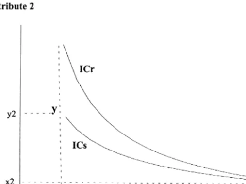
The intuition behind loss aversion is that losses loom larger than gains. Because a shift in the reference point can change losses into gains and vice versa, loss aversion can explain violations ofprocedure invariance. Figure 1 illustrates. Suppose thatx

andy are equivalent judged from reference points. That is, the gainy2− s2 is just

sufficient to offset the gainsx1− s1andx2− s2. If the reference point shifts fromsto

FIG. 1. Loss aversion.

attribute. The shift in the reference point does not affect the second attribute. Because losses loom larger than gains and no change occurs on the second attri-bute,xis now strictly preferred toy. If we draw indifference curves in Fig. 1 then loss aversion implies that the indifference curves judged from reference pointr,ICr, are

steeper than those from reference points,ICs.

Several empirical studies show support for loss aversion and closely related con-cepts as ‘‘endowment effects’’ (Kahneman, Knetsch, & Thaler, 1990) and ‘‘status quo bias’’ (Samuelson & Zeckhauser, 1988). Kühlberger (1998) gives an overview of the impact ofreference-dependence and loss aversion on risky decisions. Illustra-tions ofthe influence ofreference-dependence and loss aversion on riskless decision making can, among others, be found in Batemanet al. (1997), Herne (1998), and Tversky and Kahneman (1991).

2. THE CONTINGENT TRADE-OFF MODEL

The contingent trade-off model (Tverskyet al., 1988) generalizes standard choice theory by making preferences conditional on the response mode used. In two-attribute preference comparisons, trade-offs can either be made by using the first

(x1) or the second (x2) attribute as the response scale. Let R1 and R2 denote

the preference relation when the first and the second attribute, respectively, is used as the response scale. Fori=1, 2, Piis the asymmetric part of Riand ’i the

symmetric part. It is assumed that the Ri, i=1, 2, are weak orders that satisfy

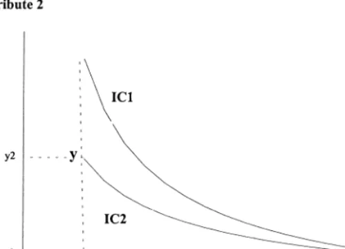
FIG. 2. Scale compatibility.

single attributes are defined as in standard choice theory. Under attribute monoto-nicity, the single-attribute preference relations are independent of the response scale used and we therefore continue to denote them by R.

The distinctive predictions of the contingent trade-off model follow from the effect of changes in the response scale. Tverskyet al. (1988) imposescale compati-bilityto explain how preferences depend on changes in the response scale (see also Fischer & Hawkins, 1993). Scale compatibility posits that an attribute becomes more important ifit is used as the response scale. Formally, scale compatibility can be defined as follows.

Definition 2 (Scale compatibility). If x, y¥X are such that for i, j¥{1, 2},

i]j, xiPyiandxjOyjthenxRjyimpliesxPiy.

Figure 2 illustrates scale compatibility. The two preference relations R1 and R2

lead to different sets of indifference curves IC1 and IC2. The indifference curves

corresponding to R1, IC1, are steeper, reflecting that the first attribute gets more

weight when it is used as the response scale. Figure 2 shows that ifx andy lie on the same indifference curve when the second attribute is used as the response scale thenx, which yields a strictly preferred level on the first attribute, lies on a higher, i.e., more preferred, indifference curve when the first attribute is used as the response scale.

Delquié (1993) gives a comprehensive overview ofthe impact ofscale compati-bility in riskless and risky decision making. His results provide strong support for scale compatibility. Two ofthe aforementioned studies provide insight into the relative sizes of the effects of loss aversion and scale compatibility. The two studies

yield conflicting results. Delquié (1993), who focused on scale compatibility, argues that the effect of scale compatibility is stronger than the effect of loss aversion. Batemanet al. (1997), whose aim was to test the influence of loss aversion, conclude that loss aversion is more effective than scale compatibility.

3. EMPIRICAL TESTS

We used a linked equivalence design to derive empirical tests ofloss aversion with scale compatibility held constant, ofscale compatibility with loss aversion held constant, and of the joint effect of loss aversion and scale compatibility. Consider two outcomes x=(x1, x2) and y=(y1, y2). Suppose that both attributes are

numerical, that higher levels are preferred to lower, and thatx2< y2. In the first

stage ofthe linked-equivalence design, three ofthe four parametersx1, x2, y1, and

y2are fixed and participants are asked to establish indifference betweenxandyby

specifying the value of the remaining parameter. Suppose that x1 is used to elicit

indifference in the first stage and denote the first-stage response byx−

1. It follows

from attribute monotonicity thatx−

1> y1. In the second stage,x

−

1is substituted and

one ofthe parameters x2, y1, and y2 is used to establish indifference, while the

remaining two parameters are held fixed at the same value as in the first stage. Standard choice theory predicts that the second-stage response should always be equal to the first-stage stimulus value. This follows immediately from transitivity and attribute monotonicity. The second-stage responses predicted by the reference-dependent model and by the contingent trade-off model can differ from the first-stage stimulus value depending on which parameter is used to elicit indifference. Table 1 gives an overview ofthe various possibilities. A formal derivation ofthese predictions is given in Appendix A. Let us note for completeness that inequalities reverse iflower levels ofan attribute are preferred to higher levels. For example, if lower levels of the first attribute are preferred to higher levels then the reference-dependent model predicts thaty1> y

'

1, wherey

'

1denotes the second-stage response.

Table 1 displays how two-attribute trade-offs can be used to test loss aversion and scale compatibility. The use ofy1to elicit indifference in the second stage of the

linked equivalence questions yields a pure test ofloss aversion. In this case, the contingent trade-off model predicts that the effect of scale compatibility is held constant. A pure test ofscale compatibility is obtained ifx2 is used to elicit the

TABLE 1

Predictionsof the Reference-Dependent Model (RDM) and the Contingent Trade-Off Model (CTO)

Parameter used in the Prediction RDM with Prediction CTO with second-stage loss aversion scale compatibility

y1 y ' 1> y1 y ' 1=y1 x2 x ' 2=x2 x ' 2> x2 y2 y' 2> y2 y ' 2< y2

second-stage response. The reference-dependent model predicts that this test will not be confounded by changes in loss aversion. Finally, the joint impact of scale compatibility and loss aversion is tested if y2 is used to elicit indifference in the

second stage. Regarding this last test, in the experiment described below we study trade-offs where scale compatibility and loss aversion make conflicting predictions. This allows a test of the relative size of the two effects.

4. MORE SPECIFIC TESTS

The models developed in Sections 1 and 2 allow us to test whether loss aversion and scale compatibility affect preferences. To make more specific predictions, further restrictions have to be imposed. First, we assume that both Rrand Ri, i=

1, 2, can be represented by utility functions Ur(x1, x2) and Ui(x1, x2), i=1, 2,

respectively. To ensure the existence ofthese representing functions Rr and

Ri must satisfy the Archimedean axiom for all r¥Xand for i=1, 2, respectively.

This requires that each bounded standard sequence is finite (Krantz, Luce, Suppes, & Tversky, 1971).

Because r=(r1, r2), we can define byri the reference level of attributei, i=1, 2.

It is assumed thatUr(x1, x2)=U(R1(x1), R2(x2))where fori=1, 2, Ri(xi)=ui(xi) −

ui(ri) ifxiRri andRi(xi)=(ui(xi) − ui(ri))/li if xiOri.

1_{Tversky and Kahneman}

1_{The illustration ofconstant loss aversion that Tversky and Kahneman (1991) give in their Fig. V} assumes thatRi(xi)=(ui(xi) − ui(ri))li ifxiOri. This is also the specification they use in their later

work. Of course, this specification is qualitatively similar to the specification we use here (letl−

i=1/li)

and none of the subsequent predictions is affected.

(1991) refer to this specification as thereference-dependent model with constant loss aversion. The parameters l_i denote the constant loss aversion coefficients for the two attributes. The functionsuiarebasic attribute utility functionsthat measure the

intrinsic value ofthe attribute levels (Köbberling & Wakker, 2000). For numerical attributes theui are assumed concave and differentiable.

Let the first attribute be numerical and such that higher levels are preferred. If the attribute levelsx2andy2 are held constant in different linked equivalence

ques-tions then we can test concavity of u1 and constant loss aversion. Let y2Px2. We

can derive two implications that permit empirical testing. The derivation ofthese tests is given in Appendix B. The first implication is that if u1 is concave then

x−

1− y1 increases with y1 in the first stage of the linked equivalence questions. If

x2Py2 and therefore x

−

1< y1, then concavity of u1 implies that x

−

1− y1 decreases

withy1. The conclusions reverse if lower levels of the first attribute are preferred.

The above results do not require constant loss aversion and also hold if li varies

withyi. The first implication therefore yields a test of concavity ofu1.

The second implication is that ifu1is concave and the reference-dependent model

with constant loss aversion holds theny'

1− y1 increases withy1. This also holds in

case x2Py2 and x

−

1< y1. The conclusions reverse iflower levels ofthe first

attribute are preferred. The second implication requires constant loss aversion. Tverskyet al. (1988) proposed the representationhi·log(x1)+log(x2)for Ri, i=

1, 2, to model scale compatibility when both attributes are numerical. The coeffi-cients h1 and h2 denote the relative weight of the first attribute when the first and

the second attribute, respectively, are used as the response scale. Because the rela-tive weights do not depend on the sizes ofx1 andx2, we refer to this model as the

contingent trade-off model with constant scale compatibility. The model predicts that

h2<h1and thath1andh2are constant across questions. Iflower levels ofattribute

iare preferred then −log(xi)is used instead oflog(xi) in the contingent trade-off

model with constant scale compatibility.

5. EXPERIMENT

Participants

Fifty-one economics students at the University Pompeu Fabra participated in the experiment. Their age was between 20 and 25 years ofage. Participants were paid 5000 pesetas (approximately $30). The experiment was carried out in two personal interview sessions. The two sessions were separated by two weeks. Before the actual experiment was administered, we tested the questionnaire in several pilot sessions. Questions

The experiment consisted ofthree groups ofquestions. We describe each group ofquestions in turn.

Group 1:Back pain questions. In the first group of questions, health status was qualitative and participants were asked to make trade-offs between years with back pain and years in full health. Questions in which health status is qualitative are commonly used in health utility measurement. It was assumed in the derivation of the empirical tests that both attributes can be used to elicit indifference. This implies that both attributes must satisfy restricted solvability to ensure that indif-ference values can always be found. Restricted solvability is unlikely to be satisfied for qualitative health states. In health utility measurement, utilities are therefore elicited by varying only the quantitative attribute, generally life duration. The impact ofscale compatibility can then not be tested, because the tests for scale compatibility require shifts in the response scale. Consequently, the first group of questions, to which we refer as the ‘‘back pain questions,’’ only tested for loss aversion. The back pain questions were included because ofthe common use of questions with qualitative health status in health utility measurement.

Back pain was described as the level of functioning on four dimensions: daily activities, selfcare activities, leisure activities, and pain. Table 2 gives the descrip-tion ofback pain. This descripdescrip-tion was taken from the Maastricht Utility

TABLE 2

The Description of Back Pain

Unable to perform some tasks at home and/or at work Able to perform all self care activities (eating, bathing, dressing)

albeit with some difficulties

Unable to participate in many types ofleisure activities Often moderate to severe pain and/or other complaints

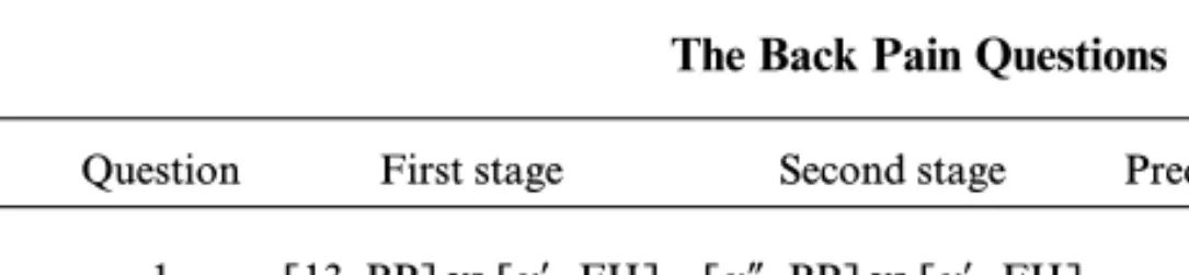
TABLE 3 The Back Pain Questions

Question First stage Second stage Prediction RDM Prediction CTO 1 [13, BP] vs [x− 1, FH] [y ' 1, BP] vs [x − 1, FH] y ' 1> 13 y ' 1=13 2 [19, BP] vs [x− 1, FH] [y ' 1, BP] vs [x − 1, FH] y ' 1> 19 y ' 1=19 3 [24, BP] vs [x− 1, FH] [y ' 1, BP] vs [x − 1, FH] y ' 1> 24 y ' 1=24 4 [31, BP] vs [x− 1, FH] [y ' 1, BP] vs [x − 1, FH] y ' 1> 31 y ' 1=31 5 [38, BP] vs [x− 1, FH] [y ' 1, BP] vs [x − 1, FH] y ' 1> 38 y ' 1=38

Measurement Questionnaire, a widely used instrument to describe health states in medical research (Rutten-van Mölken, Bakker, van Doorslaer, & van der Linden, 1995). We selected the health state back pain, because it is a familiar condition and participants were likely to know people suffering from back pain. Full health was defined as no limitations on any of the four dimensions.

Table 3 displays the five trade-offs between years with back pain and years in full health. The first attribute is life duration and the second health status (BP stands for back pain and FH for full health). A possible problem in these types of ques-tions is that people always respond in round numbers, e.g., multiples offive. To reduce this problem, we did not use multiples of five as first-stage stimulus values. We learned from the pilot sessions that participants found it hard to perceive living for very long durations which exceed their life-expectancy. Such perception problems can act against loss aversion which predicts that participants’ second-stage response should exceed the first-second-stage stimulus value. Therefore, we used life durations that were substantially lower than participants’ life-expectancy. The final columns ofTable 3 display the predicted responses according to the ref erence-dependent model with loss aversion (RDM) and the contingent trade-off model with scale compatibility (CTO). These predictions can straightforwardly be derived from Table 1.

The back pain questions also permit a test ofthe reference-dependent model with constant loss aversion. In terms ofthe analysis ofSection 4, x2Py2 and higher

amounts of the first attribute are preferred. Hence, concavity of u1 predicts that

x−

1− y1 decreases withy1 and constant loss aversion predicts thaty

'

1− y1 increases

withy1.

Group 2: Migraine questions. In the second group ofquestions, participants were asked to make trade-offs between life duration and the number of days per month they suffer from migraine. Hence, health status was quantitative and both loss aversion and scale compatibility could be tested. Table 4 gives the description ofmigraine, for which we again used the Maastricht Utility Measurement Questionnaire. Migraine was selected, because it is a relatively common disease and participants were likely to know people suffering from it.

Table 5 displays the migraine questions. The first attribute denotes life duration and the second the number ofdays per month with migraine. We avoided the use of round numbers in the first stage and used durations substantially lower than parti-cipants’ life-expectancy. Six trade-offs were asked in the first experimental session

TABLE 4

The Description of Migraine

Unable to perform normal tasks at home and/or at work Able to perform all self care activities (eating, bathing, dressing) Unable to participate in any type ofleisure activity

Severe headache

(the first stage of questions 6–11). Three questions used duration and three ques-tions used days with migraine as the response scale. In the second session, ten trade-offs were asked. Questions 6–11 are pure tests of loss aversion, questions 12 and 13 are pure tests ofscale compatibility, and questions 14 and 15 are joint tests ofloss aversion and scale compatibility in trade-offs where they make opposite predictions. Questions 12–15 used the first-stage responses from questions 8, 9, 6, and 10, respec-tively. The predictions according to the reference-dependent model with loss aver-sion and the contingent trade-off model with scale compatibility are displayed in the final two columns of the table. These predictions follow from Table 1. Ques-tions 12 and 13 permit a test ofthe contingent trade-offmodel with constant scale compatibility.

Group 3: Car accident questions. In the third group ofquestions, health status was again quantitative. Participants were told to imagine that they had experienced a car accident as a result ofwhich they are temporarily unable to walk. To restore their ability to walk, participants had to undergo rehabilitation therapy for some time. Rehabilitation sessions last 2 h per day and result in moderate to severe pain for a couple of hours following the rehabilitation sessions. Participants were asked to elicit indifference between two types of therapy, described as intensive and less intensive therapy. The two types of therapy differ in the time that elapses until par-ticipants are able to walk again and the number ofhours ofpain following the rehabilitation sessions.

Table 6 displays the car accident questions. The first attribute denotes years until being able to walk again and the second the number ofhours ofpain after the

TABLE 5 The Migraine Questions

Question First stage Second stage Prediction RDM Prediction CTO 6 [16, 3] vs [x− 1, 8] [y ' 1, 3] vs [x − 1, 8] y ' 1> 16 y ' 1=16 7 [19, 8] vs [x− 1, 4] [y ' 1, 8] vs [x − 1, 4] y ' 1> 19 y ' 1=19 8 [34, 13] vs [x− 1, 4] [y ' 1, 13] vs [x − 1, 4] y ' 1> 34 y ' 1=34 9 [22, 4] vs [28,x− 2] [22,y ' 2] vs [28,x − 2] y ' 2< 4 y ' 2=4 10 [26, 8] vs [17,x− 2] [26,y ' 2] vs [17,x − 2] y ' 2< 8 y ' 2=8 11 [32, 8] vs [20,x− 2] [32,y ' 2] vs [20,x − 2] y ' 2< 8 y ' 2=8 12 [34, 13] vs [x− 1,4] [34, 13] vs [x − 1,x ' 2] x ' 2=4 4 <x ' 2< 13 13 [22, 4] vs [28,x− 2] [22, 4] vs [x ' 1,x − 2] x ' 1=28 22 <x ' 1< 28 14 [16, 3] vs [x− 1,8] [16,y ' 2] vs [x − 1, 8] y ' 2< 3 3 <y ' 2< 8 15 [26, 8] vs [17,x− 2] [y ' 1, 8] vs [17,x − 2] y ' 1> 26 17 <y ' 1< 26

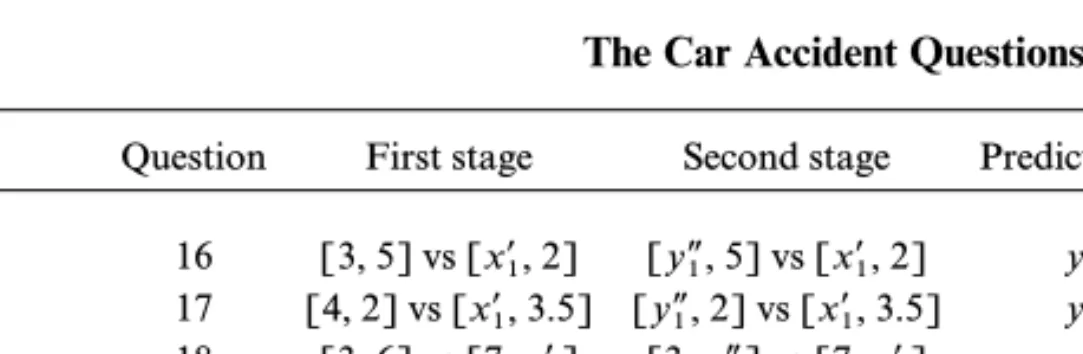
TABLE 6 The Car Accident Questions

Question First stage Second stage Prediction RDM Prediction CTO 16 [3, 5] vs [x− 1, 2] [y ' 1, 5] vs [x − 1, 2] y ' 1< 3 y ' 1=3 17 [4, 2] vs [x− 1, 3.5] [y ' 1, 2] vs [x − 1, 3.5] y ' 1< 4 y ' 1=4 18 [3, 6] vs [7,x− 2] [3,y ' 2] vs [7,x − 2] y ' 2< 6 y ' 2=6 19 [5, 2] vs [1.5,x− 2] [5,y ' 2] vs [1.5,x − 2] y ' 2< 2 y ' 2=2 20 [3, 5] vs [x− 1, 2] [3, 5] vs [x − 1,x ' 2] x ' 2=5 2 <x ' 2< 5 21 [5, 2] vs [1.5,x− 2] [5, 2] vs [x ' 1,x − 2] x ' 1=1.5 1.5 <x ' 1< 5 22 [4, 2] vs [x− 1,3.5] [4,y ' 2] vs [x − 1, 3.5] y ' 2< 2 2 <y ' 2< 3.5 23 [3, 6] vs [7,x− 2] [y ' 1, 6] vs [7,x − 2] y ' 1< 3 3 <y ' 1< 7

rehabilitation sessions. Four trade-offs were asked in the first experimental session (the first stage of questions 16–19) and eight in the second. Questions 16-19 are pure tests ofloss aversion, questions 20 and 21 pure tests ofscale compatibility, and questions 22 and 23 joint tests of loss aversion and scale compatibility in trade-offs where they make opposite predictions. Questions 20–23 used the first-stage responses from questions 16, 19, 17, and 18, respectively. The predictions according to the reference-dependent model with loss aversion and the contingent trade-off model with scale compatibility are displayed in the final two columns of the table. These predictions follow from Table 1. The pure scale compatibility questions 20 and 21 permit a test ofthe contingent trade-offmodel with constant scale compati-bility.

Methods

To avoid order effects, we varied the order in which the three groups of questions were administered. Similarly, within each group the order ofthe questions was varied. Recruitment ofparticipants took place one week before the actual experi-ment started. At recruitexperi-ment, participants were handed three practice questions, one from each group. Participants were asked to answer these practice questions at home before coming to the experiment. This procedure was intended to familiarize participants with the questions. Prior to each group ofquestions, participants were asked whether they had experienced any problems in answering the practice ques-tion that corresponded to that group. Participants were then asked to explain their answer to the practice question. This procedure allowed us to test whether partici-pants had understood the questions. In case we were not convinced that a participant had understood a question, we went over the task again until we were convinced that he or she understood the task.

Appendix C shows the formulation of the back pain questions. A similar format was used for the migraine questions and the car accident questions. Indifferences were elicited by a choice bracketing procedure. Participants reported their answers by filling in a table. At any time during the interview, participants were allowed to check earlier responses and to adjust these ifdesired. It is crucial for our test ofthe

reference-dependent model that participants interpret the option in which both parameters are given as their reference point. We took special care to formulate the questions in such a way that ambiguities about the reference point were ruled out. We consistently referred to the option in which both parameters were given as the participant’s current health state and to the option in which a parameter had to be specified as the health state to which the participant could change to. The choice-bracketing procedure used three answer categories: ‘‘I prefer my current health state,’’ ‘‘I want to change to the other health state,’’ and ‘‘I am indifferent between my current health state and a change to the other health state.’’ To try and avoid response errors, the participants were asked after each question to confirm the elicited indifference value. The final comparison was displayed once again and par-ticipants were asked whether they agreed that the two options were equivalent. In case they did not agree, we restarted the choice-bracketing procedure.

The trade-offs used in this study are hypothetical. We do not believe that the hypothetical nature ofthe outcomes is problematic. Several studies showed that people’s responses do not differ in a systematic way between hypothetical and real tasks (Beattie & Loomes, 1997; Camerer, 1995; Camerer & Hogarth, 1999; Tversky & Kahneman, 1992). Previous studies on loss aversion demonstrated its effect on preferences both in hypothetical (Jones-Lee, Loomes, & Philips, 1995; McDaniels, 1992; Samuelson & Zeckhauser, 1988; Tversky & Kahneman, 1986) and in real tasks (Batemanet al., 1997; Tversky & Kahneman 1991).

Differences between second-stage responses and first-stage stimulus values were examined both by the parameteric t-test and by the nonparametric Wilcoxon test for matched-pairs. Since the results were qualitatively similar only the results for the t-test are reported. Tests ofproportions ofparticipants who behaved according to a particular model were performed by the standard Z-test. The contingent trade-off model with constant scale compatibility was estimated by linear regression. Only the second-stage equivalence questions could be used in the estimation because in the first-stage either the dependent or the independent variable displays no varia-tion. Questions 12 and 20 yielded estimates ofh2and questions 13 and 21 ofh1. The

specification of the contingent trade-off model with constant scale compatibility was tested by the RESET test (Ramsey, 1969).

6. RESULTS

One participant was excluded from the analyses because he did not answer all questions. Because the tests ofloss aversion and scale compatibility require attri-bute monotonicity, those participants who violated attriattri-bute monotonicity were excluded in each ofthe groups ofquestions. This left 42, 46, and 38 participants in the analyses ofthe back pain, migraine, and car accident questions, respectively. Most excluded participants violated attribute monotonicity only once. In terms of questions, attribute monotonicity was violated in 7% ofthe questions. To examine the robustness ofthe results, we also analyzed the data by excluding only those questions in which attribute monotonicity was violated. This had no significant impact on the results.

Pure Tests of Loss Aversion

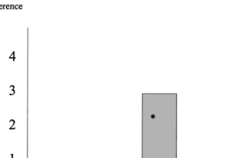
Back pain questions. Figure 3 shows the difference between the second-stage response and the first-stage stimulus value for the five back pain questions. The solid arrows display the direction of the difference that is predicted by the reference-dependent model with loss aversion. Stars indicate statistical significance at

a=0.05. The figure shows significant evidence of loss aversion in agreement with the reference-dependent model with loss aversion.

In Section 4, we derived two tests ofthe reference-dependent model with constant loss aversion. Concavity ofu1 is supported by the data. The difference betweenx

−

1

and y1 decreases with y1 in agreement with the concavity of u1 (the correlation

betweenx−

1− y1 andy1is equal to −0.646 and is significantly different from zero at

a=0.01). The data do not support constant loss aversion. The difference between

y'

1 and y1 decreases with y1 contrary to the prediction ofthe reference-dependent

model with constant loss aversion (the correlation between y'

1− y1 andy1 is equal

to − 0.259 and is significantly different from zero ata=0.01).

An explanation for why loss aversion decreases with life duration ( y1) may be

that the substitutability of health status and life duration increases with life dura-tion. Empirical studies showed that loss aversion decreases with increases in substi-tutability (Chapman, 1998; Ortona & Scacciati, 1992). McNeil, Weichselbaum, and Pauker (1981) found that the substitutability between health status and life duration increases with life duration. They observed that people are unwilling to trade life duration for improved health status if life duration is low. Hence, for low life duration preferences over life duration and health status are lexicographic. If life duration

increases beyond a certain number ofyears, however, people are willing to trade-off life duration and health status and this willingness increases with life duration (see also Miyamoto & Eraker, 1988; Pliskin, Shepard, & Weinstein, 1980).

At the individual level, we find that most participants do not behave consistently according to the reference-dependent model with loss aversion. Thirteen partici-pants areuniformly loss averse, i.e., they behave according to the predictions ofthe reference-dependent model with loss aversion in each question. One participant is uniformly gain seeking, i.e., he or she behaves contrary to the predictions ofthe reference-dependent model with loss aversion in each question. This preference pattern implies that the participant gives more weight to gains than to losses ofthe same size, hence the term gain seeking. No participant isuniformly loss neutral, i.e., equally sensitive to gains and losses in all questions. The remaining 28 subjects display a mixed pattern ofresponses. The proportion ofloss averse participants is significantly higher than the proportion of gain seeking participants in questions 1, 2, and 3. There is no significant difference in questions 4 and 5.

Migraine questions. Figure 4 shows the results ofthe migraine questions. Note from Table 5 that life duration increases in questions 6–8. Hence, we observe again that the degree ofloss aversion decreases with life duration. The pattern observed in questions 9–11 is mixed. There appears to be no obvious factor that explains why loss aversion varies over questions 9–11. Therefore, it cannot be excluded that the variation is primarily due to response error, even though it is unlikely that response error would lead to a significant bias in the wrong direction as in question 9.

The mixed evidence with respect to loss aversion is reflected in the individual data. Only two participants are uniformly loss averse. The other 44 participants

display a mixed pattern ofbehavior; no participant is uniformly gain seeking or uniformly loss neutral. The proportion of loss averse participants is significantly higher than the proportion ofgain seeking participants in questions 6, 7, and 10. It is significantly lower in question 9. Hence, we observe again that for most partici-pants the effect of loss aversion is not constant but varies over questions.

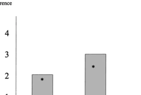
Car accident questions. Figure 5 shows the results ofthe car accident questions. The reference-dependent model with loss aversion predicts a negative difference in each question, as indicated by the solid arrows. This prediction is confirmed, but the difference between second-stage response and first-stage stimulus value is signi-ficant in just two questions. At the individual level, we observe again that most participants do not behave consistently according to the reference-dependent model with loss aversion, but that there are trade-offs in which participants are loss averse and trade-offs in which participants are gain seeking. Six participants are uniformly loss averse. The other participants display a mixed pattern ofbehavior; no partici-pant is uniformly gain seeking or uniformly loss neutral. The proportion of loss averse participants is significantly higher than the proportion of gain seeking participants in questions 16, 18, and 19.

Pure Tests of Scale Compatibility

Both the migraine questions and the car accident questions contained two pure tests of scale compatibility. Figure 6 displays the difference between the second-stage response and the first-second-stage stimulus value. The open arrows indicate the direction of the difference predicted by the contingent trade-off model with scale compatibility. Three out of four tests support the contingent trade-off model with

FIG. 6. Pure tests ofscale compatibility.

scale compatibility. In question 13, however, the bias is in the opposite direction. Hence, we observe mixed results on scale compatibility in the migraine questions.

Only one participant behaves uniformly according to the contingent trade-off model with scale compatibility, i.e., responses are in the direction predicted by the model in all four questions. All other participants display a mixed pattern of behavior: none behaves uniformly opposite to the contingent trade-off model with scale compatibility, i.e., the participant gives consistently more weight to the attri-bute that is not used as the response scale, and none is uniformly insensitive to the response scale used. The proportion ofparticipants whose behavior is consistent with the contingent trade-off model with scale compatibility is significantly higher than the proportion ofparticipants whose behavior is inconsistent with the con-tingent trade-off model with scale compatibility in questions 12, 20, and 21. It is significantly lower in question 13.

Table 7 shows the estimation results for the contingent trade-off model with constant scale compatibility. We find that h₁>h₂ as predicted by the model.

TABLE 7

The Estimation Results for the Contingent Trade-Off Model with Constant Scale Compatibility

Estimate F-statistic RESET test Question (standard error) (P value)

12 h2=1.349 (0.125) 12.744 (P < 0.01) 13 h1=2.092 (0.131) 9.255 (P < 0.01) 20 h2=1.534 (0.124) 2.821 (P > 0.05) 21 h1=2.533 (0.181) 210.034 (P < 0.01)

FIG. 7. Joint tests ofloss aversion and scale compatibility.

However, the RESET test rejects the null hypothesis ofcorrect model specification in all but one case. Hence, the data are not consistent with the contingent trade-off model with constant scale compatibility.

Joint Tests of Loss Aversion and Scale Compatibility

Figure 7 shows the results ofthe four tests ofthe joint impact ofloss aversion and scale compatibility. As before, solid arrows indicate the predictions of the reference-dependent model with loss aversion and open arrows the predictions ofthe contingent trade-offmodel with scale compatibility. Figure 7 shows that the relative sizes of the effects of loss aversion and scale compatibility are trade-offdependent. In three tests the bias is in the direction ofloss aversion and in one test in the direction of scale compatibility. The difference is only significant in question 15.

The individual data confirm that the relative sizes of the biases due to loss aver-sion and scale compatibility are not constant but vary over trade-offs. There are only two participants for whom the effect of loss aversion dominates the effect of scale compatibility in all four questions. There is no participant for whom the effect of scale compatibility dominates the effect of loss aversion in all four questions. The proportion of participants for whom the effect of loss aversion dominates is signi-ficantly higher than the proportion of participants for whom the effect of scale compatibility dominates in question 15. There is no significant difference in the other questions.

7. CONCLUSION

A first conclusion is that loss aversion and scale compatibility are robust. There is significant evidence of loss aversion and scale compatibility in most trade-offs

even though we used tests that avoid confounding the effects of loss aversion and scale compatibility, examined loss aversion and scale compatibility in a new domain, and used an experimental design that was not a priori conducive to viola-tions of procedure invariance. Second, the effects of loss aversion and scale compa-tibility are not constant but vary over trade-offs. The data are inconsistent with models of constant loss aversion and constant scale compatibility. Third, the effects ofloss aversion and scale compatibility vary within individuals. Few participants behave consistently according to loss aversion or scale compatibility or both. This latter finding suggests that loss aversion and scale compatibility are primarily manifest at the aggregate level and less at the individual level. It cannot be excluded, however, that this finding is partly due to response errors in spite of the care we took in eliciting responses.

The robustness ofloss aversion and scale compatibility emphasizes the need to build descriptive models of decision making that incorporate these effects. The findings of this paper show that the modeling of these effects may be complicated. Previous models typically treated loss aversion and scale compatibility as constant (Bowman, Minehart, & Rabin, 1999; Shalev, 1997; Tverskyet al., 1988; Tversky & Kahneman, 1991). Our data are consistent neither with the reference-dependent model with constant loss aversion nor with the contingent trade-off model with constant scale compatibility.

Broadly speaking, two viewpoints can be distinguished regarding the relevance of loss aversion and scale compatibility for prescriptive decision analysis. The first viewpoint argues that loss aversion and scale compatibility have relevance for prescriptive decision analysis, because they influence the way people think about and later experience outcomes and thus reflect people’s true preferences. According to this point of view, prescriptive models must be built that are sufficiently detailed to incorporate loss aversion and scale compatibility, so that these effects can be taken into account in prescriptive decision analyses. The implications ofour research for this viewpoint are similar to the implications described above for the descriptive models: the task ofdeveloping such models may be complicated given that the simplifying assumptions of constant loss aversion and constant scale compatibility do not appear to hold.

The second point ofview is that loss aversion and scale compatibility are biases that should be avoided in prescriptive decision analysis. Loss aversion and scale compatibility cause preferences to violate procedure invariance. Procedure invariance is a crucial assumption ofprescriptive decision analysis and, hence, ways must be sought to eliminate the impact ofloss aversion and scale compatibility. The overall message of the paper is positive for this point of view. The findings that loss aversion and scale compatibility vary over decision contexts and at the individual level suggest that it may be possible to identify decision contexts that are hardly affected by these biases. The joint tests of loss aversion and scale compatibility suggest that there are decision contexts in which the effects of loss aversion and scale compatibility approximately offset each other. The identification of decision contexts in which the (joint) effects of loss aversion and scale compatibility are minimal may allow the measurement ofutilities without the distorting impact of loss aversion and scale compatibility. For example, our results suggest that health

utility measurement should rely on trade-offs between health status and life dura-tion in which life duradura-tion is relatively long, because the effect of loss aversion decreases with life duration and appears to vanish for longer life durations.

APPENDIX A: DERIVATION OF THE EMPIRICAL TESTS OF SECTION 3

Throughout this appendix superscriptsŒ_andœ_{denote first-stage and second-stage}

responses, respectively. We consider three cases depending on which parameter is used to elicit indifference in the second stage. Recall that it is assumed that on both attributes higher levels are preferred to lower levels and thatx2< y2.

Case1: y1 is used to elicit indifference in the second stage. In this case the first

attribute is still used as the response scale, but the outcome in which both param-eters are held fixed changes fromy=(y1, y2)tox=(x

−

1, x2). The contingent

trade-off model predicts that y'

1=y1, because the response scale does not change and,

thus, the second stage yields(x−

1, x2)’1( y

'

1, y2).y

'

1=y1 then follows from

transi-tivity of ’1and attribute monotonicity.

According to the reference-dependent model, the reference point shifts fromyto

xand the second stage elicits (x−

1, x2)’x( y

'

1, y2). Let zdenote the point(x

−

1, y2).

By loss aversion, the first-stage indifference(x−

1, x2)’y( y1, y2)implies that(x

−

1, x2)

Pz( y1, y2). Let (x

−

1, x2)’z(z1, y2). Such a z1 exists by restricted solvability. By

attribute monotonicity z1> y1. Loss aversion also implies that if ( y

' 1, y2)’x (x− 1, x2) then ( y ' 1, y2)Pz(x − 1, x2). By transitivity, ( y ' 1, y2)Pz(z1, y2) and by attribute monotonicityy' 1> z1> y1.

Case 2: x2 is used to elicit indifference in the second stage. In this case, y=

( y1, y2) is still the outcome in which both parameters are given, but the response

scale changes from the first to the second attribute. The reference-dependent model predicts that x'

2=x2. This follows straightforwardly from transitivity of ’y,

attri-bute monotonicity, and the second-stage indifference(x−

1, x

'

2)’y( y1, y2).

According to the contingent trade-off model, the second stage elicits (x−

1, x

'

2)

’₂( y1, y2). By attribute monotonicity, y2> x

'

2 and thus by scale compatibility

(x−

1, x

'

2)P1( y1, y2). The first stage yielded (x

− 1, x2)’1( y1, y2) and hence (x − 1, x ' 2) P₁(x−

1, x2)by transitivity of R1. Attribute monotonicity implies thatx

'

2> x2.

Case3: y2 is used to elicit indifference in the second stage. In this case, there is

both a shift in the reference point fromy=(y1, y2) to x=(x

−

1, x2) and a change

in the attribute that is used as the response scale. We show that the reference-dependent model and the contingent trade-off model yield conflicting predictions. The reference-dependent model predicts that y'

2 > y2. Let z denote the point

(x−

1, y2). By loss aversion, the first-stage indifference (x

−

1, x2)’y( y1, y2) implies

that (x−

1, x2)Pz( y1, y2). Let z2 be such that (x

−

1, x2)’z( y1, z2). z2 exists by

restricted solvability. z2> y2 by attribute monotonicity. Loss aversion implies

that if (x− 1, x2)’x( y1, y ' 2) then ( y1, y ' 2)Pz(x −

1, x2). Transitivity implies that

( y1, y

'

2)Pz( y1, z2). Attribute monotonicity implies thaty

'

2> z2> y2.

According to the contingent trade-off model, the second stage elicits

( y1, y ' 2)’2(x − 1, x2). y '

(x− 1, x2)P1( y1, y ' 2). (x − 1, x2)P1( y1, y '

2) and the first-stage indifference

(x− 1, x2)’1( y1, y2) imply that ( y1, y2)P1( y1, y ' 2) by transitivity of R1. Hence, y2> y ' 2 by attribute monotonicity.

APPENDIX B: DERIVATION OF THE EMPIRICAL TESTS OF SECTION 4

Suppose thatx2 andy2 are held constant in the linked equivalence questions. In

the first stagex−

1 is elicited, hence y=(y1, y2)is the reference point and the

indi-vidual determinesUy(x

−

1, x2)=Uy( y1, y2)=U(R1(x1), R2(x2)). Note thatU(0, 0)=

0. This holds regardless ofwhether loss aversion is constant. Becausex2 andy2 are

held constant, R2(x2) is constant. By attribute monotonicity, R1(x

−

1) must be a

constant for all y1¥X1. If R1(x

− 1)=u1(x − 1) − u1( y1), then u1(x − 1) − u1( y1)=z= constant. Letu−

1denote the first derivative ofuwith respect to the first attribute. By

a first order Taylor series approximation u1(x

− 1)=u1( y1)+(x − 1− y1) · u − 1( y1). Thus x− 1− y1=(u1(x − 1) − u1( y1))/u − 1( y1)=z/u −

1( y1) which increases with y1 by the

con-cavity of u1. It is easily verified that if x2Py2 and thereforex

−

1< y1 then x

−

1− y1

decreases withy1. To derive this letRi(xi)=ui(xi) − ui(ri)ifxiOri and let the loss

aversion be reflected inRi(xi)ifxiRri. This model is just a rescaling ofthe model

considered above. The same line ofargument as above can now be applied. The above conclusions reverse ifthe first attribute is such that lower amounts are preferred.

At the second stage, x=(x−

1, x2) is the reference point and y

'

1 is set such that

Ux(x − 1, x2)=Ux( y ' 1, y2)=U(R1( y '

1), R2( y2)). Becausex2 andy2 are held constant,

R2( y2)is constant and by attribute monotonicityR1( y

'

1)is constant for allx

−

1¥X1.

Let the reference-dependent model with constant loss aversion hold. Then

R1( y ' 1)=(u1( y ' 1) − u1(x −

1))/l1 is constant. Because loss aversion is constant,

u1( y

'

1) − u1(x

−

1)=c=constant. At the first stage of the linked equivalence design

we found thatu1(x

−

1) − u1( y1)=z=constant. It follows that for ally1¥X1, u1( y

'

1) −

u1( y1)=c+z=constant.c+z > 0by loss aversion (see Table 1).u1( y

'

1)=u1( y1)+

( y'

1− y1) · u

−

1( y1) by a first order Taylor series approximation and thus

y' 1− y1=(u1( y ' 1) − u1( y1))/u − 1( y1)=(c+z)/u −

1( y1) which increases withy1 by the

concavity of u1. This conclusion also holds in case x2Py2 and x

−

1< y1. The

conclusion is reversed iflower amounts ofthe first attribute are preferred.

APPENDIX C: FORMULATION OF THE BACK PAIN QUESTIONS

Suppose that you have 13 more years to live with back pain. In this question you are asked to state the number ofyears in full health that you consider equivalent to living for 13 more years with back pain. That is, you have to determine the number Y that makes the following two options equivalent:

1. Living for 13 years with back pain. After these 13 years you die. 2. Living for Y years in full health. After these Y years you die. Use the following table to answer this question.

Your current You can change

situation is 1 to situation 2 Decision Years with Years in full I am indifferent

Step back pain health I remain in 1 between 1 and 2 I change to 2

1 13 13 2 13 0 3 13 11 4 13 2 5 13 9 6 13 4 7 13 7 8 13 5 REFERENCES

Bateman, I., Munro, A., Rhodes, B., Starmer, C., & Sugden, R. (1997). A test ofthe theory of reference-dependent preferences.Quarterly Journal of Economics,62, 479–505.

Beattie, J. & Loomes, G. (1997). The impact ofincentives upon risky choice experiments.Journal of Risk and Uncertainty,14, 155–168.

Bostic, R., Herrnstein, R. J., & Luce, R. D. (1990). The effect on the preference reversal of using choice indifferences.Journal of Economic Behavior and Organization,13, 193–212.

Bowman, D., Minehart, D., & Rabin, M. (1999). Loss aversion in a consumption-savings model.Journal of Economic Behavior and Organization,38, 155–178.

Camerer, C. F. (1995). Individual decision making. In J. Kagel and A. Roth (Eds.),The handbook of experimental economics(pp. 587–703). Princeton, NJ: Princeton Univ. Press.

Camerer, C. F., & Hogarth, R. M., (1999). The effects of financial incentives in experiments: A review and capital-labor-production framework.Journal of Risk and Uncertainty,19, 7–42.

Chapman, G. B. (1998). Similarity and reluctance to trade.Journal of Behavioral Decision Making,11, 47–58.

Delquié, P. (1993). Inconsistent trade-offs between attributes: New evidence in preference assessment biases.Management Science,39, 1382–1395.

Delquié, P. (1997). ‘Bi-matching’: A new preference assessment method to reduce compatibility effects. Management Science,43, 640–658.

Fischer, G.W., & Hawkins, S. A. (1993). Strategy compatibility, scale compatibility, and the prominence effect.Journal of Experimental Psychology: Human Perception and Performance,19, 580–597. Herne, K. (1998). Testing the reference-dependent model: An experiment on asymmetrically dominated

reference points.Journal of Behavioral Decision Making,11, 181–192.

Jones-Lee, M. W., Loomes, G., & Philips, P. R. (1995). Valuing the prevention ofnon-fatal road injuries: Contingent valuation vs. standard gambles.Oxford Economic Papers,47, 676–695.

Kahneman, D., Knetsch, J. L., & Thaler, R. H. (1990). Experimental test of the endowment effect and the Coase theorem.Journal of Political Economy,98, 1325–1348.

Köbberling, V., & Wakker, P. P. (2000). An Index ofLoss Aversion. Working Paper, University of Maastricht.

Krantz, D. H., Luce, R. D., Suppes, P., & Tversky, A. (1971).Foundations of measurement(Vol. 1). New York: Academic Press.

Kühlberger, A. (1998). The influence of framing on risky decisions: A meta-analysis.Organizational Behavior and Human Decision Processes,75, 23–55.

McDaniels, T. L. (1992). Reference points, loss aversion, and contingent values for auto safety.Journal of Risk and Uncertainty,5, 187–200.

McNeil, B. J., Weichselbaum, R., & Pauker, S. G. (1981). Tradeoffs between quality and quantity of life in laryngeal cancer.New England Journal of Medicine,305, 982–987.

Miyamoto, J. M., & Eraker, S. A. (1988). A multiplicative model ofthe utility ofsurvival duration and health quality.Journal of Experimental Psychology: General,117, 3–20.

Ortona, G., & Scacciati, F. (1992). New experiments of the endowment effect.Journal of Economic Psychology,13, 277–296.

Pliskin, J. S., Shepard, D. S., & Weinstein, M. C. (1980). Utility functions for life years and health status.Operations Research,28, 206–223.

Ramsey, J. B. (1969). Tests for specification errors in classical linear least squares analysis.Journal of the Royal Statistical Society, Series B,31, 350–371.

Rutten-van Mölken, M. P., Bakker, C. H., van Doorslaer, E. K. A., & van der Linden, S. (1995). Methodological issues ofpatient utility measurement: Experience from two clinical trials. Medical Care,33, 922–937.

Samuelson, W., & Zeckhauser, R. (1988). Status quo bias in decision making.Journal of Risk and Uncertainty,1, 7–59.

Shalev, J. (1997). Loss aversion in a multi-period model.Mathematical Social Sciences,33, 203–226. Slovic, P. (1975). Choice between equally valued alternatives. Journal of Experimental Psychology:

Human Perception and Performance,1, 280–287.

Tversky, A., & Kahneman, D. (1986). Rational choice and the framing of decisions. Journal of Business,59, 251–278.

Tversky, A., & Kahneman, D. (1991). Loss aversion in riskless choice: A reference-dependent model. Quarterly Journal of Economics,56, 1039–1061.

Tversky, A., & Kahneman, D. (1992). Advances in prospect theory: Cumulative representation of uncertainty.Journal of Risk and Uncertainty,5, 297–323.

Tversky, A., Sattath S., & Slovic, P. (1988). Contingent weighting in judgment and choice.Psychological Review,95, 371–384.