computing
J. Yang,1 S. Cong,1,∗ X. Liu,2 Z. Li,2 and K. Li3
1Department of Automation,University of Science and Technology of China, Hefei 230027, P. R. China 2
Department of Physics, University of Science and Technology of China, Hefei 230026, P. R.China
3
Imperial College London, MRC Institute of Medical Sciences, London, W12 0NN, UK
The number of measurements required to reconstruct the states of quantum systems increases ex-ponentially with the quantum system dimensions, which makes the state reconstruction of high-qubit quantum systems have a great challenge in physical quantum computing experiments. Compres-sive sensing (CS) has been verified as a effective technique in the reconstruction of quantum state, however, it is still unknown that if CS can reconstruct quantum states given the less data measured by nuclear magnetic resonance (NMR). In this paper, we propose an effective NMR quantum state reconstruction method based on CS. Different from the conventional CS-based quantum state re-construction, our method uses the actual observation data from NMR experiments rather than the data measured by the Pauli operators. We implement measurements on quantum states in practical NMR computing experiments and reconstruct states of 2,3,4 qubits using fewer number of measure-ments, respectively. The proposed method is easy to implement and performs more efficiently with the increase of the system dimension size. The performance reveals both efficiency and accuracy, which provides an alternative for the quantum state reconstruction in practical NMR.
I. INTRODUCTION
Nuclear magnetic resonance (NMR) is one of the most promising physical methods to realize quantum comput-ing, which has attracted tremendous interest in both the physics and information science community [1–4]. In practical NMR quantum computing experiments, the reconstruction of quantum states occupies an impor-tant position. Conventional quantum state tomography (QST) is a common method for NMR quantum state re-construction (QSR)[5–7], which requires complete mea-surements of the quantum state to be reconstructed. For ann-qubit stateρ, the number of complete measurements is d2 = 4n. This number increases exponentially with n, and makes the reconstruction work of the high-qubit NMR state becomes extremely difficult as n is large. In order to reduce the number of measurements, people sometimes use local quantum tomography [8] to recon-struct the states. However, local quantum tomography requires a sufficient amount of prior information before reconstructing, which does not have universal applica-bility. Therefore, the reconstruction of high-qubit NMR quantum states has great challenge.
Compressed sensing (CS) [9] has attracted a great in-terest as an effective approach of recovering sparse sig-nals. This approach is now widely applied in many fields, such as image processing [10, 12], wireless communication [11], nuclear magnetic resonance imaging (MRI) [13, 14] and NMR spectroscopy [15, 16]. CS also provides a new idea to solve the problem of high-qubit quantum state re-construction. People have performed accurate quantum state reconstruction in physical systems such as photon [17–19] and ion trap [20]. However, it is still not clear that if CS can reconstruct quantum states provided mea-surement data from NMR, because in NMR the
measure-ments of QSR are obtained in a different way. In practical NMR computing experiments, the signal of each mea-surement is sampled in the time-domain and then trans-ferred into a frequency-domain spectrum. The spectrum contains a number of resonance peaks, and each peak is associated with an observableOi of the system. The
observables of the same spectrum constitute an NMR ob-servable group, which can be measured simultaneously. When reconstructing an actual NMR state ρ based on CS, due to the particularity of practical NMR measure-ments, the observables should be sampled in units of ob-servable groups rather than individual obob-servablesOi ,
which is different from the sampling method in conven-tional CS-based QST [21–23]. Moreover, the CS opti-mization problem requires an appropriate optiopti-mization algorithm. The most commonly used optimization algo-rithms in CS are LS [24], Dantzig [25], gradient projection [26] and so on. Li and Cong first applied the ADMM al-gorithm to QSR and showed that the ADMM alal-gorithm has better performance than the commonly used algo-rithms [27, 28]. FP-ADMM algorithm was proposed by Zheng et al. [29], which combines the fixed point idea and ADMM algorithm and improves further the efficiency of the reconstruction.
In this paper, we show that CS is an effective tech-nique for the NMR quantum state reconstruction. To our knowledge, we carry out the first experimental re-construction of NMR states by using CS. We theoret-ically prove that CS can be applied to the reconstruc-tion of actual NMR quantum states, and give the de-tailed reconstruction steps, which combines CS and the characteristics of the practical NMR measurement. FP-ADMM is used as the optimization algorithm to solve the CS optimization problem. We experimentally verify the proposed method by the reconstruction of actual NMR
states with 2,3,4 qubits and analyze the effects of factors on the reconstruction performance. The experimental results show that the proposed method can effectively reconstruct the NMR quantum state using only a small amount of measurement data. The reconstruction per-formance reveals both efficiency and accuracy with the increase of system dimension size. The proposed method is easily applicable to higher qubits for any NMR low-rank quantum states.
The structure of this paper is as follows. In Sec. II, after a brief introduction to the practical NMR measure-ment method, the CS theory and the FP-ADMM algo-rithm, we prove our reconstruction method and give spe-cific steps of the method. In Sec. III, the experimental reconstruction results are shown. We perform reconstruc-tion of actual 2,3,4 qubits NMR states, respectively, and analyze the reconstruction performance through contrast experiments. The conclusion of this paper is given in Sec. IV.
II. QUANTUM STATE RECONSTRUCTION BASED ON COMPRESSIVE SENSING AND
ACTUAL NMR OBSERVATION DATA
As an indirect measurement process, the system to be measured in NMR is an n-qubit quantum state consist-ing of spin nuclei in the sample solution under a con-stantz-direction magnetic fieldB0. There is a magnetic moment of the spin nuclei in the magnetic field, whose direction is same as B0 and magnitude is proportional to the angular momentum of the spin. The external control field is a radio frequency (RF) pulse magnetic field on the x−y plane. When applying an RF pulse consisting of a plurality of resonant frequencies to the sample solution, the nuclei absorbs the energy of the RF pulse, and the angle between the magnetic moment and B0 changes, leading to a Larmor precession of the nu-clei. There is an induction coil winding on the surface of the sample solution, and the nuclear precession results in a free induction decay current signal s(t) in the in-duction coil: s(t) = P
iM0eiΩite−t/T2, where t stands for time, Ωi denotes the resonant frequencies, and i is
the flag,M0 is the value of fixed RF field magnetization intensity vector, and T2 represents the transverse relax-ation time. S(ω) is a frequency-domain spectrum which is obtained from the Fourier transform of s(t): S(ω) =
R∞
0 s(t)e
−iωtdt = A(ω) + iB(ω) where ω stands for
the frequency, andA(ω) =P
iKT2−1 . (ω−Ωi) 2 +T2−2 and B(ω) = P iK(ω−Ωi) . (ω−Ωi) 2 +T2−2 are the real and imaginary parts of S(ω) , respectively. The spectrum ofA(ω) andB(ω) near the resonant frequency Ωi are resonance peaks, with the peaks of A(ω) being
absorption peaks and that ofB(ω) being symmetric dis-persion peaks.
When measuring an n-qubit quantum state ρ whose dimension isd = 2n, each resonance peak in S(ω) cor-responds to an observableOi, and the observation value
of Oi is proportional to the area of the signals in the
corresponding peak ofA(ω): hOii= 1 P0 Z Ωi+∆ω Ωi−∆ω A(ω)dω, (1)
whereP0 is the scaling factor which can be determined by the peak0s area of the eigenstate in the same sample solution, and ∆ω is a fixed range value, which ensures all signals of the selected formant are included in the frequency range [Ωi−∆ω,Ωi+ ∆ω].
As the spectrum S(ω) contains d resonance peaks, the observation data of the correspondingdobservables are obtained simultaneously in one NMR measurement. Suchdobservables constitute an NMR observable group, defined asOkj =Ok1, O2k, ..., Odk , wherej= 1,2, ..., d,
and k = 1,2, ..., v is the serial number of the group. Herevdenotes the total number of the observable groups which is determined by the composition of the experi-mental sample and the actual measurement scheme. For example, Ok
j represents the j-th observable in the k
-th group and is also expressed in -the subscript form as Ok
j =Okj. {Oi} (i= 1,2, ..., vd) is the set of all the
ob-servables. In practical NMR experiments, people design a measurement scheme of v different NMR observable groups to measure the complete observables of ρ, with some inevitably repetitive or linearly related observables in different groups, meaning that the total observables of
{Oi} are over-complete forρ.
Because the observables of {Oi} are over-complete,
a conventional method for NMR QST is to per-form the following transper-formation: based on the d observables Ojk in each group Ojk , Ojk can be transformed into a set of measurement operators
Mk j = Mk 1, M2k, ..., Mdk by Mjk = P2n−1 i hijO k j, where Mk
j is an n-qubit Pauli operator that is
the tensor product of Pauli matrices {I, X, Y, Z} =
1 0 0 1 , 0 1 1 0 , 0 −i i 0 , 1 0 0 −1 , and hij
are the elements in the transformation matrixHof
Ok j
and
Mk
j . Each column ofH represents a linear
trans-formation from Okj to one operator of Mjk . The observation values Ojk can also be transformed to measured valuesMjk . It is easy forMjk to remove all the repetitions and get a complete set of measurement operators{Mm} (m= 1,2, ..., d2), thus one can directly
calculate the reconstructed density matrix ˆρof the state ρwith {Mm}and {hMmi}: ˆρ= 21n
P4n
m=1(hMmi ·Mm).
However, as the number of qubits increases, the number of measurement operators required for quantum tomog-raphy increases exponentially, and the corresponding ac-tual NMR measurement becomes extremely cumbersome.
Here we propose an effective reconstruction method of the actual NMR quantum states based on CS, in which we directly use observables{Oi}but not the transformed
measurement operators{Mm}. One necessary condition
of using CS in QSR is that the density matrix ofρshould be low-rank. That is, the rank ofρis much less than its dimension: rd. In practical NMR quantum comput-ing experiments, the quantum state to be reconstructed is mostly pure or nearly pure, which satisfies the low-rank condition. Therefore, CS can be applied to the re-construction of actual NMR quantum states. The recon-struction process can be described as to solve the follow-ing convex optimization problem:
minkρk∗, s.t.y=A·vec(ρ), (2) wherekρk∗is the nuclear norm ofρ, which equals to the sum of singular values, vec(·) represents the transforma-tion from a matrix to a vector by stacking the matrix0s columns in order on the top of one another. The sam-pling matrixAis the matrix form of the all the sampled observablesOi, and the sampling vectory is the vector
form of the corresponding observation valueshOii.
Considering the measurement method in NMR experi-ment, the observable groupsOkj and the corresponding actual observation valuesOkj are randomly sampled for the CS-QSR. Because the observation values are sam-pled in groups, here we defined a new sampling rate as
ηg=g/v, (3)
wheregis the number of the sampled groups, andvis the total number of groups. It is worth mentioning thatηg
is different from the general sampling rate ηm =m
d2 , where m and d2 represent the sampled number and total number of the measurement operators {Mm},
re-spectively, andηg, ηm∈[0,1].
Without loss of generality, assuming that the randomly sampled serial number is from 1 to g, then A and y in NMR can be written as A= vec(O1j )T vec( O2 j )T .. . vec( Ogj )T /√d, (4) and y= O1j , O2j ,· · ·, Ogj T, (5) where vec( Ok
j )T represents the transformation from
the d observables of
Ok
j to d horizontal vectors
ar-ranged in vertical order: vec( n Ok j o )T= vec(Ok 1)T vec(Ok 2)T . . . vec(Ok d)T , and
yis the vector of the observation values corresponding to
the observables ofA. In this case, the optimization prob-lem (2) is an equation group composed ofg×dequations. It should be noted that, since the total observables are over-complete, there may be some repeating equations in (2), but this repetition does not affect the solution of (2). Candes et al. proved that, if the sampling matrix A satisfies the rank restricted isometry property (RIP) [30], the convex optimization problem (2) has a unique opti-mal solution equaling to the true density matrix [31]. It is proved that the sampling matrix A consisting of randomly sampled Pauli measurement operators satisfies rank RIP with very high probability [25]. Since the trans-formation between the operators ofOjk andMjk is linear, if the sampling matrixAM consisting ofgdifferent
Pauli measurement operator groups
Mk
j satisfies rank
RIP, then the sampling matrixAO that consists of
cor-respondingg observable groups
Ok
j also satisfies rank
RIP. This means, in theory, our method sampling the ob-servable groups
Ok
j is applicable to the reconstruction
of actual NMR quantum stateρ.
In this paper, we use the FP-ADMM algorithm pro-posed by Zheng et al.[29] to solve the optimization prob-lem (2). The iterative steps of the FP-ADMM algorithm are as follows: ρk1+1=D δ1 µ (mat((I−δA†A)vec(ρk 1)+δA†(y−A·vec(Sk)−Y k µ ))) ρk+1=12(ρk1+1+ ρk1+1 † ) Sk+1=S δλ µ
(mat((I−δA†A)vec(Sk)+δA†(y−A·vec(ρk+1)−Yk
µ )))
Yk+1=Yk+µ
A·vec(ρk+1+Sk+1)−y
(6)
where S is a sparse matrix representing interference terms, which is updated alternatively with ρ in the it-erative process, mat(·) is the inverse operator of mat(·), Dλ(X) is the singular value contraction operator defined
as Dλ(X) = U Sλ(S)VT, where U SVT is the singular
value decomposition ofX, andSλ(X) is the soft
thresh-old defined as[Sλ(X)]ij= xi j−λ,ifxi j> λ xi j+λ,ifxi j< λ 0, otherwise . Y ∈Rmis
the Lagrange multiplier, andδ∈[0,+∞] is the iterative step size,λ, µ >0. In the reconstruction experiments of this paper, the parameters of FP-ADMM algorithm are selected as follows: δ= 1,λ= 1/√d[27],µ= 0.5/kykF, the initial values ofρ,S and Y are taken as zero matri-ces. The stopping criterion of the FP-ADMM algorithm isy−A·vec(ρk+Sk)
F/kykF < ε1 or the number of iterationsk > kmax, letε1= 10−7 andkmax= 30.
In general, the process of reconstructing NMR quan-tum states with the method proposed can be summarized as follows: Randomly sample a certain number of
Ok j
and
Ok
j , construct the convex optimization problem
(2) with the sampled Ojk and Okj , and solve (2) with the compressive FP-ADMM algorithm. The final optimal solution ˆρis the reconstruction result of the state ρ.
reconstruction and is defined as: f = Tr ˆρρ†.p
Tr ( ˆρ2) Tr (ρ2), (7) where ˆρandρrepresent the experimentally reconstructed density matrix and the corresponding ideal density ma-trix, respectively, andf ∈[0,1].
III. EXPERIMENTAL STATES
RECONSTRUCTION IN NMR AND ANALYSIS
We implement practical NMR experiments to recon-struct the states of n = 2,3,4 qubits, respectively, in order to examine the reduction performance of the number of measurements of our method. The experi-ments are carried out on a Bruker AV-400 spectrome-ter (9.4 T) at a room temperature of 303.0 K [8]. The physical systems of n = 2,3,4 qubits states are 1 3C-labeled chloroform (CHCL3) dissolved in deuterated ace-tone, Diethyl-fluoromalonate (C7H11FO4 ) dissolved in 2H-labeled chloroform, and iodotrifiuoroethylene (C
2F3I) dissolved in d-chloroform, respectively. One 1H and one 13C are used for the first and second qubit ofn= 2, and one 1H, 13C and 19F are used for the first, second and third qubit of n= 3. For n = 4, one 13C is labeled as the first qubit, and 19F1, 19F3 and 19F3 as the second, third, and fourth qubits, respectively. The systems are first prepared into pseudopure states (PPS) using the line selective-transition method [32] in the experiment device. Then, by adjusting the pulse RF, the pseudo-pure states are manipulated into the target quantum state|ψ2i,|ψ3i and|ψ4i[7, 8].
The state vectors associated with these three kinds of states are: |ψ2i=|00i, (8) |ψ3i= 4 5|000i − 3 5|001i, (9) |ψ4i= 1 √ 2(|0101i+|1010i), (10) in which |0i = 1 0 and |1i = 0 1 represent the ground state and the excited state of the nucleus, re-spectively. |ψ2i is an eigenstate, and |ψ3i and |ψ4i are superposition states.
Let ρ2 =|ψ2i hψ2|, ρ3 =|ψ3i hψ3| and ρ4 =|ψ4i hψ4| be the corresponding density matrices of |ψ2i, |ψ3i and
|ψ4i. In order to accurately reconstruct ρ2, ρ3 and ρ4, the states |ψ2i, |ψ3i and |ψ4i need to be prepared and observed repeatedly for the complete observation data. In practical NMR experiments, the total number of ob-servable groups required arev2 = 6,v3 = 16 andv4 = 44
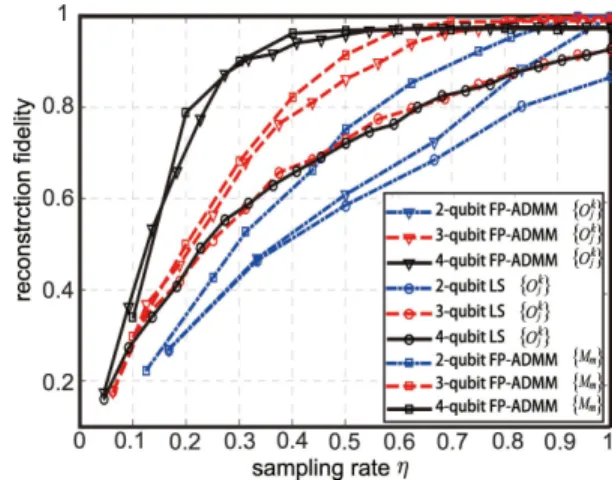
FIG. 1. The experimental results of reconstruction fidelities ofρ2,ρ3and ρ4 with different sampling rates in three differ-ent cases. The blue dot-dash line, red dashed line and black solid line correspond toρ2, ρ3 and ρ4, and the triangle, cir-cle and square mark correspond to the cases of A, B and C, respectively. For case A and B, the incremental step of sam-pling rates are selected as ∆ηg = 1/6,1/16 and 1/22 ofρ2,ρ3 andρ4, respectively, and for case C the incremental step of sampling rate is fixed as ∆ηm= 0.1.
forn= 2,3,4, respectively. The corresponding numbers of observables in each group ared2= 22= 4,d3= 23= 8 andd4= 24= 16. Thus, the total number of observables
Oi for |ψ2i, |ψ3iand |ψ4iare 6×4 = 24, 16×8 = 128 and 44×16 = 704, respectively, which are significantly larger than the theoretical number of complete measure-ment operatorsd2, being 16, 64 and 256 forn = 2,3,4, respectively.
The ability of reconstructing quantum states using less sampling rate is significant for the proposed method. We do the experiments to demonstrate this ability in differ-ent cases. We carry out the experimdiffer-ents for 3 scenarios using two optimal algorithms and two kinds of sampling matrices for the comparisons: Randomly sampling from the observable groups
Ok
j by using (A) compressive
FP-ADMM algorithm and (B) LS algorithm; (C) Ran-domly sampling from the measurement operatorsMmby
using compressive FP-ADMM algorithm. The sampling rateηg in (3) is usually used to demonstrate the
reduc-tion performance of the number of the observable groups
Okj , andηm=m
d2 is used for the measurement op-erators{Mm}. The performance of state reconstruction
is the fidelity in (7). Under each sampling rate, we construct each state 100 times and average over the re-sulting fidelities as the final average fidelity favg. The
experimental results of reconstruction fidelities ofρ2, ρ3 and ρ4 with different sampling rates in three cases are shown in Fig.1.
It can be seen from Fig. 1 that: All the reconstruc-tion fidelities increases with the increase of the sam-pling rate. The average fidelities of FP-ADMM algo-rithm reach approximately 1 and remain stable when
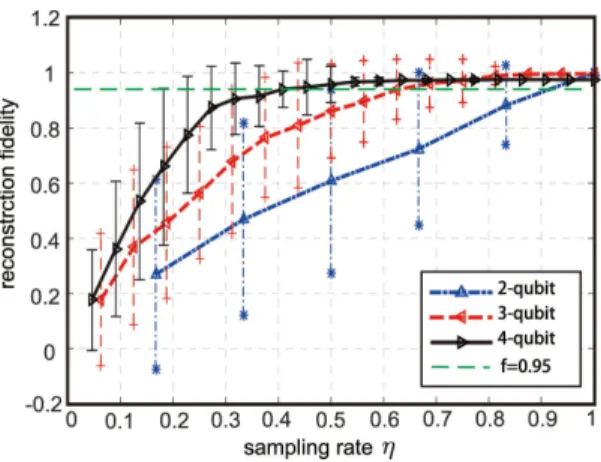
FIG. 2. The reconstruction average fidelity and mean square errorζat different sampling rates using the proposed method. The blue dot-dash line with the inverted triangle, the red dash line with the left triangle, and the black solid line with the right triangle correspond toρ2,ρ3 andρ4 respectively, while the star, plus and dash symbol represent the corresponding error bars. The green dash line represents the reconstruction fidelity f= 0.95. The length of the error bar represents the mean square error of 100 experimental reconstruction fideli-ties.
the corresponding sampling ratesηgreach around 1, 0.75
and 0.5 withn =2, 3 and 4, respectively. However, the maximum fidelities of LS with n =2, 3 and 4 are only favg−LS ∼0.87, 0.93and0.93 when ηm = 1. The
com-pressive FP-ADMM algorithm is obviously better than the LS algorithm in the performance of state reconstruc-tion. For the two kinds of sampling matrices
Ok j and
{Mm} using compressive FP-ADMM algorithm, the
re-construction fidelity ofOkj is slightly worse than that of Mm whenn= 2, but becomes close when n= 3 and
shows almost the same performance when n = 4. This experimental result shows that the proposed method per-forms more efficiently with the increase of the system di-mension size, which can be use to the state reconstruction of high-qubit quantum state in NMR.
The mean square error not only reflects the degree of discretization of the fidelities, but also responds to suc-cess probability of reconstruction at the corresponding sampling rate. We also do the experiments to study the mean square error of the fidelity at the different sam-pling rates of the proposed method with samsam-pling matri-ces
Ok
j using compressive FP-ADMM algorithm. Here
we use ζ to represent the value of mean square error. In the experiments, we choose f ≥0.95 as the criterion that the reconstruction is successful. When the average fidelity is near 0.95, the smaller of ζ, the more concen-trated the fidelity distribution, and the higher the suc-cess probability of reconstruction, and vice versa. The reconstruction average fidelity and mean square error ζ at different sampling rates using the proposed method are shown in Fig. 2.
Figure 2 shows that the mean square error ζ de-creases with the increase of qubit number at the same
sampling rate, e.g, the mean square errors are ζ = 0.33,0.17and0.07 of n=2, 3 and 4 with ηg = 0.5. ζ also
tends to decrease with the increase of ηg at the same
qubit number.
We set the mean square errors ζ ≤0.1 to get a suffi-ciently large success probabilities of reconstruction (the probability that f ≥ 0.95 ). The least sampling rates forζ ≤0.1 of n=2, 3 and 4 are ηg = 1, 0.75 and0.5 ,
with the mean square errors beingζ= 0, 0.08and0.07, respectively. The least sampling rates are decreasing with the increase of qubit number. The average fi-delities of reconstruction at these sampling rates are favg= 1.0, 0.97and0.96 and the corresponding success
probabilities of reconstruction are 100%, 92% and 97%. This experimental results show that, we can carry out high-probability reconstruction of the quantum states in NMR with rather low sampling rates sing the proposed method, especially for high-qubit quantum states.
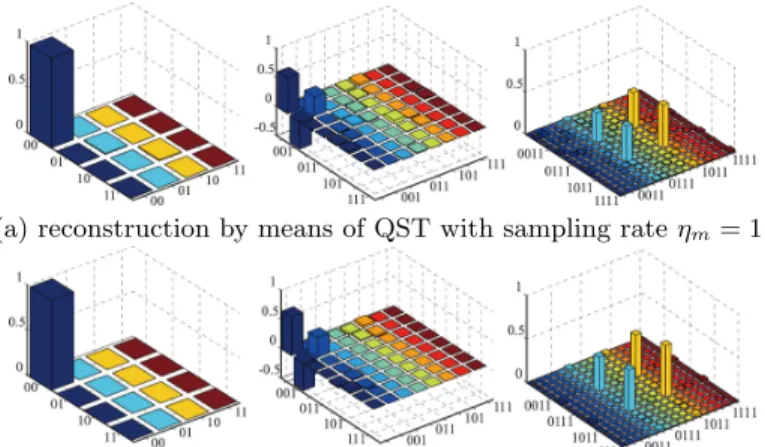
The experimental results of reconstructed density ma-trices ofρ2,ρ3andρ4are shown in Fig. 3, and the fideli-ties of the reconstructed density matrices in Figs. 3 (a) and (b) are shown in Table 1. In order to ensure a suffi-ciently high success probability of reconstruction, accord-ing to the experimental results of Fig. 2, we choose the sampling rates ofρ2,ρ3 and ρ4 as ηg2= 1.0,ηg3= 0.75 and ηg4 = 0.50, with the corresponding sampling rates beingg2= 6,g3= 12 andg4= 22.
One can see from Table 1 that: The reconstruc-tion fidelities by quantum state tomography are 0.9942, 0.9838 and 0.9606, respectively. And the reconstruc-tion fidelities by the proposed method are 0.9999, 0.9896 and 0.9679, respectively, which have better performances than those of QST, indicating that our CS-QSR method is robust to the noise and interference in the actual mea-surement data to a certain extent. The important thing is the sampling rates (number of sampled groups) used in our method are also much less than 1 when the qubit number n≥3. The experimental results show that our method can reconstruct the actual NMR quantum states more accurately and effectively with only a small amount of observation data directly. The method proposed in this paper is the optimal reconstruction method under the ex-isting conditions and can instruct the reconstructions of high-qubit quantum states in NMR.
Fidelity ρ2 ρ3 ρ4 QST 0.9942 0.9838 0.9606 Our method 0.9999 0.9896 0.9679
TABLE I. The fidelities of the reconstructed density matrices in Fig. 3 (a) and (b).
(a) reconstruction by means of QST with sampling rateηm= 1
(b) reconstruction by the proposed method with the sampling ratesηg2= 1.0,ηg3= 0.75 andηg4= 0.50
FIG. 3. The experimental results of reconstructed density matrices ofρ2,ρ3andρ4. (a) is the reconstruction by means of QST with sampling rateηm= 1, and (b) is the reconstruc-tion by the proposed method. The three histograms from left to right in (a) and (b) correspond to the reconstructed den-sity matrices of ρ2, ρ3 and ρ4, respectively. Only the real parts of the reconstructed density matrices are given and the imaginary parts are ignored, because the imaginary parts of the elements in the ideal density matricesρ2,ρ3 andρ4 are all 0.
IV. CONCLUSION
In this paper, we first reconstructed actual NMR quan-tum states via compressive sensing. We also proposed an effective NMR quantum state reconstruction method based on CS and gave a detailed derivation of the method in both theoretical and experimental aspects. The obser-vation data is directly used in our method so as to save the transformation process of QST, which effectively en-hances the efficiency of the state reconstruction in prac-tical NMR experiments. We validated our method with actual observation data of different qubit states and an-alyzed the effect of different factors on the reconstruc-tion performance. The method proposed in this paper is both feasible in implementation and accurate in re-construction and can greatly reduce the number of mea-surements required, which provides a new protocol for the state reconstruction with higher qubits in practical NMR experiments.
ACKNOWLEDGMENTS
This work was supported by the National Natural Sci-ence Foundation of China (61573330).
∗
[1] J.A. Jones and M. Mosca, J. Chem. Phys. 109, 1648 (1998).
[2] I. L. Chuang, L. M. K. Vandersypen, X. Zhou, D. W. Leung and S. Lloyd, Nature,393, 143 (1998).
[3] L. M. K. Vandersypen, M. Steffen, G. Breyta, C. S. Yan-noni, M. H. Sherwood and I. L. Chuang, Nature, 414, 883 (2001).
[4] C. Negrevergne, T. S. Mahesh, C. A. Ryan, M. Ditty, F. Cyr-Racine, W. Power, N. Boulant, T. Havel, D. G. Cory, and R. Laflamme, Phys. Rev. Lett.96, 170501 (2006). [5] G.L. Long, H.Y. Yan, Y.S. Li, C.C. Tu, J.X. Tao, H.M.
Chen, M.L. Liu, X. Zhang, J. Luo, L. Xiao and X.Z. Zeng, Phys. Lett. A286, 121 (2001).
[6] J. S. Lee, Phys. Lett. A305, 349 (2002).
[7] Z. Li, M. H. Yung, H. Chen, D. Lu, J. D. Whitfield, X. Peng, A. Aspuru-Guzik and J. Du, Sci. Rep.1, 88 (2010). [8] J. Pan, Y. Cao, X. Yao, Z. Li, C. Ju, H. Chen, X. Peng,
S. Kais and J. Du, Phys. Rev. A89, 022313 (2014). [9] E. J. Cands, J. Romberg and T. Tao, IEEE Trans. Inf.
Theory52, 489 (2006).
[10] M. Lustig, D. Donoho, and J. M. Pauly, Magn. Reson. Med.58, 1182 (2007).
[11] S. Stankovi?, I. Orovi? and L. Stankovi?, Signal Process-ing104, 43 (2014).
[12] P. Sen and S. Darabi, IEEE Trans. Vis. Comput. Graph.
17, 487 (2011).
[13] M. Lustig, D. Donoho and J. M. Pauly, Magn. Reson. Med.58, 1182 (2007).
[14] M. L. Maguire, S. Geethanath, C. A. Lygate, V. D. Kodibagkar and J. E. Schneider, J. Cardiovasc. Magn. r.17, 45 (2015).
[15] X. Andrade, J. N. Sanders and A. Aspuru-Guzik. P. NATL. ACAD. SCI. USA.109, 13928 (2012).
[16] D. J. Holland, M. J. Bostock, L. F. Gladden and D. Ni-etlispach, Angew. Chem. Int. Edit.50, 6548 (2011). [17] D. Gross, Y. K. Liu, S. T. Flammia, S. Becker and J.
Eisert, Phys. Rev. Lett.105, 150401 (2010).
[18] A. Shabani, R. L. Kosut, M. Mohseni, H. Rabitz, M. A. Broome, M. P. Almeida, A. Fedrizzi and A. G. White Phys. Rev. Lett.106, 100401 (2011).
[19] W. T. Liu, T. Zhang, J. Y. Liu, P. X. Chen, and J. M. Yuan, Phys. Rev. Lett.108, 170403 (2012).
[20] C. Schwemmer, G. Tth, A. Niggebaum, T. Moroder, D. Gross, O. Ghne and H. Weinfurter, Phys. Rev. Lett.113, 040503 (2014).
[21] S. T. Flammia, D. Gross, Y. K. Liu and J. Eisert, New J. Phys.14, 095022(2012).
[22] T. Heinosaari, L. Mazzarella, M. M. Wolf, Commun. Math. Phys.318, 355 (2013).
[23] C. J. Mioss, R. von Borries, M. Argaez, L. Velzquez, C. Quintero and C. M. Potes, IEEE T. Signal Process.57, 2424 (2009).
[24] A. Smith, C. A. Riofro, B. E. Anderson, H. Sosa-Martinez, I. H. Deutsch and P. S. Jessen, Phys. Rev. A87, 030102 (2013).
[25] Y. K. Liu,in Advances in Neural Information Processing Systems, pp: 1638-1646 (2011).
[26] M. A. T. Figueiredo, R. D. Nowak and S. J. Wright, IEEE Journal of selected topics in signal processing, IEEE. J. Sel. Top. Signal Process.1, 586 (2007).
[27] K. Li and S. Cong, in The 19th World Congress of the IFAC (2014) pp. 6878-6883.
[28] K. Li, K. Zheng, J. Yang, S. Cong, X. Liu and Z. Li, Quantum Information Processing, Accepted (2017).
[29] K. Zheng, K. Li, and S. Cong, Sci. Rep.6, 38497 (2016). [30] E. J. Candes and T. Tao, IEEE Trans. Inf. Theory 59,
4203 (2005).
[31] E. J. Candes, C. R. Math.346, 589 (2008).
[32] X. Peng, X. Zhu, X. Fang, M. Feng, K. Gao, X. Yang and M. Liu, Chem. Phys. Lett.340, 509 (2001).