Design and development of a continuous, open-return transonic wind tunnel facility

(1)

DESIGN AND DEVELOPMENT OF A CONTINUOUS, OPEN-RETURN TRANSONIC WIND TUNNEL FACILITY

BY CODY GRAY

THESIS

Submitted in partial fulfillment of the requirements for the degree of Master of Science in Aerospace Engineering

in the Graduate College of the

University of Illinois at Urbana-Champaign, 2017

Urbana, Illinois Adviser:

(2)

ii

Abstract

A new transonic wind tunnel facility was designed and built on the University of Illinois at Urbana-Champaign campus to enhance testing capabilities of the transonic flow regime. The new tunnel will expand the experimental capabilities available to the Department of Aerospace Engineering at UIUC for studying and understanding topics such as compressible dynamic stall aerodynamics, shock buffet phenomenon and control, shock wave boundary layer ingestion to a propulsor, and other future research topics.

The new wind tunnel is a rectangular testing facility with a 6 in (width) x 9 in (height) cross-sectional area in the test section. It is a continuous, open-return facility, capable of operating within a Mach number range of M=0-0.8, and possibly reaching M=0.85 or higher depending on the test section configuration. The wind tunnel was assembled and installed in the Aerodynamics Research Laboratory. The tunnel is driven by a centrifugal blower that exhausts the air back into the laboratory. The components designed for the tunnel were the nozzle, diffuser, test section, settling chamber, inlet flow conditioning section, and the structural assembly.

The most significant challenges in the design and development of the tunnel were enveloped in the test section and suction plenum control system. When performing experiments on transonic aerodynamic bodies, if the Mach number is high enough, pockets of locally supersonic flow will be seen in the test section. Therefore, to simulate unbounded transonic flight, partially-open test section walls were implemented to prevent shock reflections and test section choking. The suction across these walls was controlled by flaps at the aft end of the test section. The pressure differential created across the open-area walls can cause vibrational issues if adequate suction is not provided and unloaded into the diffuser via control flaps. For this reason, thicker open-area walls were substituted after the testing with thinner walls experienced these undesirable vibrations.

(3)

iii

Acknowledgements

This project would not be complete without the support and guidance that I received from my adviser Prof. Phil Ansell. He has been incredibly helpful throughout the design and development process and I have enjoyed my time working under his supervision.

I would like to thank my family for all the love and support they have shown me throughout my time here at UIUC. I am forever grateful for my family and I hope to make you all proud in the next steps of my career. I would also like to thank Prof. Jim Leylek from the University of Arkansas for all the guidance through my final undergraduate years, especially for convincing me to apply to his alma mater, UIUC.

I am also grateful to the machine shop guys, Greg, Lee, Steve, and Dustin, without whom this tunnel could not have been built. Finally, I would like to thank all the members for the aerodynamics research group, especially Aaron Perry, for all the help during the completion of this project.

(4)

iv

List of Figures

Fig. 1.1 a) Airfoil in subsonic flow regime; b) airfoil in transonic flow regime; c) airfoil in

supersonic flow regime.2 ... 2

Fig. 1.2 Transonic wind tunnel schematic. ... 3

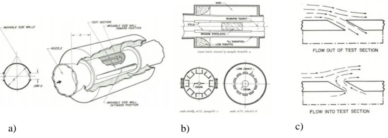
Fig. 1.3 a) Slanted walls test section configuration; b) slotted walls test section configuration; c) perforated walls test section configuration.1_{... 4}

Fig. 2.1 Comparison of pressure recovery and volume flow envelopes for a notional axial fan and centrifugal blower. ... 8

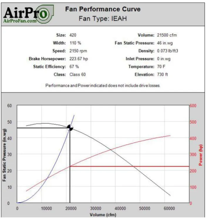
Fig. 2.2 Performance curve of AirPro Fan model 420, sized for transonic wind tunnel. ... 9

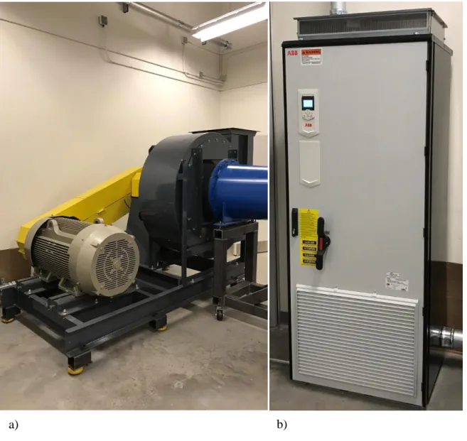
Fig. 2.3 a) AirPro blower system; b) ABB VFD. ... 10

Fig. 2.4 a) Inlet nozzle side view; b) inlet nozzle isometric view. ... 12

Fig. 2.5 3D inlet geometry for calculating contraction ratio.9 ... 13

Fig. 2.6 Schematic of match point location.10 ... 14

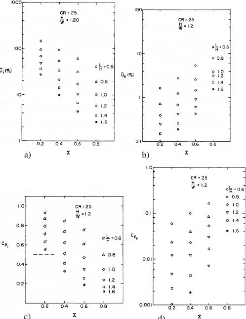
Fig. 2.7 a) Entrance velocity variation chart; b) exit velocity variation chart; c) entrance pressure coefficient chart; d) exit pressure coefficient chart.10 ... 16

Fig. 2.8 3D CAD model of settling chamber. ... 18

Fig. 2.9 a) Circular honeycomb; b) square honeycomb; c) hexagonal honeycomb.20 ... 19

Fig. 2.10 Settling chamber panels with slots: top and bottom walls. ... 22

Fig. 2.11 Screen tensioning system... 23

Fig. 2.12 a) Turbulence screen assembly; b) screen L-stock and flatbar frame. ... 24

Fig. 2.13 a) Honeycomb assembly; b) honeycomb L-stock frame. ... 24

Fig. 2.14 Settling chamber corner bracket. ... 25

Fig. 2.15 a) PVC entrance; b) PVC entrance attached to settling chamber. ... 26

Fig. 2.16 a) Settling chamber access door; b) bolting bracket to seal access door. ... 27

Fig. 2.17 a) Diffuser side view; b) diffuser isometric view. ... 29

Fig. 2.18 Diffuser FEA: Von Mises stress. ... 31

Fig. 2.19 Diffuser FEA: displacement in X-direction. ... 31

Fig. 2.20 3D isometric view of test section. ... 32

Fig. 2.21 a) Mach number distribution with perforated walls; b) Mach number distribution with slotted walls. ... 34

(7)

vii

Fig. 2.22 Comparison of perforated walls with straight holes and inclined holes at different

open-area ratios.1 ... 35

Fig. 2.23 Cross-flow characteristics of perforated walls with 60 degree inclined holes for various ratios of hole diameter to wall thickness, open-area ratio 6% at M=0.90.1 ... 35

Fig. 2.24 Hole inclination orientation.1_{... 36}

Fig. 2.25 Porous plate model. ... 37

Fig. 2.26 Porous plate with laser slot and static pressure ports. ... 37

Fig. 2.27 Suction plenum attached to test section. ... 38

Fig. 2.28 Plenum to diffuser gap. ... 39

Fig. 2.29 Suction plenum equipped with laser sheet window... 39

Fig. 2.30 Diffuser suction control flaps schematic.1 ... 40

Fig. 2.31 Diffuser suction control flap design cross section. ... 41

Fig. 2.32 3D model of choke vane mechanism. ... 42

Fig. 2.33 a) Choke vane top view; b) choke vane side view. ... 42

Fig. 2.34 Isometric view of test section walls. ... 44

Fig. 2.35 Custom square tube bolting bracket. ... 44

Fig. 2.36 Rectangular plate moment factor.5 ... 45

Fig. 2.37 Test section side wall window. ... 46

Fig. 2.38 Laser sheet window. ... 47

Fig. 2.39 Airfoil mount FEA: displacement in the Y-direction. ... 48

Fig. 2.40 Airfoil mount apparatus. ... 49

Fig. 2.41 Test section pressure transducer and tap. ... 52

Fig. 2.42 LabVIEW data acquisition block diagram. ... 53

Fig. 2.43 LabVIEW front panel for Mach number calculation. ... 53

Fig. 2.44 LabVIEW front panel for test section temperature, speed of sound, and velocity calculation. ... 53

Fig. 2.45 Static pressure tabs on both sides of porous wall. ... 54

Fig. 2.46 Structural assembly... 55

Fig. 2.47 Custom leveling bolt assembly for settling chamber support... 56

Fig. 2.48 Leveling mount for nozzle and diffuser. ... 57

(8)

viii

Fig. 2.50 Nozzle to test section transition with gap. ... 59

Fig. 2.51 Nozzle to test section transition after smoothing process... 59

Fig. 3.1 Mach number distribution vs fan RPM. ... 61

Fig. 3.2 CFD inlet boundary condition. ... 63

Fig. 3.3 CFD outlet boundary condition. ... 63

Fig. 3.4 CFD wall boundary condition. ... 64

Fig. 3.5 CFD viscous model. ... 65

Fig. 3.6 a) CFD solution initialization; b) CFD reference values. ... 66

Fig. 3.7 CFD velocity magnitude along centerline plane in streamwise downstream Z-direction. ... 67

Fig. 3.8 CFD velocity along centerline plane in streamwise downstream Z-direction. ... 68

Fig. 3.9 CFD velocity along centerline plane in vertical Y-direction. ... 68

Fig. 3.10 CFD velocity magnitude for full 3D tunnel mesh. ... 69

Fig. 3.11 CFD velocity magnitude on centerline plane in streamwise downstream Z-direction, displaying the boundary layer. ... 69

Fig. 3.12 CFD static pressure along centerline plane in streamwise downstream Z-direction. .... 70

Fig. 3.13 CFD static pressure plot along centerline plane in streamwise downstream Z-direction. ... 70

Fig. 3.14 CFD static pressure plot along walls in streamwise downstream Z-direction. ... 70

Fig. 3.15 CFD residuals plot to show converging solution. ... 71

Fig. A. 1 AirPro dimension diagram.7... 74

Fig. A. 2 ABB ACS880 VFD dimensions. ... 75

Fig. B. 1 Test section side wall connector, nozzle side. ... 76

Fig. B. 2 Test section side wall connector, diffuser side. ... 77

Fig. B. 3 Test section to nozzle flange. ... 78

Fig. B. 4 Test section side wall. ... 79

Fig. B. 5 Test section top and bottom upstream wall. ... 80

Fig. B. 6 Test section to diffuser flange. ... 81

Fig. B. 7 Test section window frame. ... 82

Fig. B. 8 Test section window frame with isometric view. ... 83

(9)

ix

Fig. B. 10 Diffuser. ... 85

Fig. B. 11 Nozzle front and side. ... 86

Fig. B. 12 Nozzle back and bottom. ... 87

Fig. B. 13 Choke vane. ... 88

Fig. B. 14 Suction control flaps. ... 89

Fig. B. 15 Airfoil mount. ... 90

Fig. B. 16 Motor mount left. ... 91

Fig. B. 17 Motor mount left. ... 92

Fig. B. 18 Motor mount extension. ... 93

Fig. B. 19 Motor mount right. ... 94

Fig. B. 20 Motor mount right. ... 95

Fig. B. 21 Laser sheet window frame. ... 96

Fig. B. 22 Laser sheet window frame with isometric view. ... 97

Fig. B. 23 Laser sheet window glass. ... 98

Fig. B. 24 Porous plate. ... 99

Fig. B. 25 Porous plate with slot. ... 100

Fig. B. 26 Suction plenum. ... 101

Fig. B. 27 Suction plenum with isometric view. ... 102

(10)

x

List of Tables

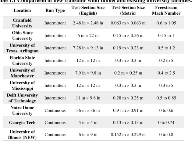
Table 1.1 Comparison of new transonic wind tunnel and existing university facilities. ... 6

Table 2.1 Screen configurations.11 ... 21

Table 3.1 Transonic wind tunnel performance characteristics. ... 61

(11)

xi

Nomenclature

List of Symbols

a speed of sound

A cross-section area

Ad,e cross-section area of the diffuser exit plane Ats cross-section area of the wind tunnel test section A* cross-section area at choked conditions

β porosity or open-area ratio

B moment factor

CD wing drag coefficient

CL wing lift coefficient

Cp pressure coefficient

D drag force or diameter

DH hydraulic diameter

∆𝑝 pressure change

e exit plane

𝜀0𝑒𝑞 equivalent free-stream turbulence

𝜀𝑠∗ intrinsic turbulence created by the screen in the optimum position

𝜀_∗ minimum value of turbulence

γ specific heat ratio

H height

i inlet plane

k pressure drop coefficient

Kh pressure loss coefficent

L lift force or length

𝑚̇ mass flow rate

M Mach number

Mmax maximum moment

M∞ free stream Mach number

(12)

xii

P static pressure

PT total pressure

q dynamic pressure

q∞ free-steam dynamic pressure

ρ density

R universal gas constant

s length of short side

S airfoil reference area

Smax maximum allowable stress

t window thickness

T static temperature

TT total temperature

U mean velocity

Um average velocity

𝑢̃ percentage of maximum variation in velocity

V velocity

Vcl centerline velocity

Vcor velocity at corners

Vd,e velocity at the diffuser exit plane

Vmax maximum velocity

Vmin minimum velocity

Vts test section velocity

𝑣̇ volumetric flow rate

(13)

xiii

List of Abbreviations

AoA angle of attack

CAD computer aided design

CFD computational fluid dynamics

CFM cubic feet per minute

CR contraction ratio

FEA finite element analysis

hp horse power

ID inside diameter

OD outer diameter

PIV particle image velocimetry

psi pounds per square inch

RPM revolutions per minute

RTV room temperature vulcanization

SIS shock-induced separation

(14)

1

Chapter 1 Introduction

Transonic wind tunnel testing encompasses the speed range between Mach 0.8-1.2, the transition between subsonic to supersonic speeds. Operation so close to the speed of sound, M=1.0, presents unusual challenges both in the design of aircraft and wind tunnels.1 This difficulty is caused by the aerodynamic phenomenon where the flow changes from a “single-type flow,” purely subsonic or supersonic, to a “mixed-type flow” with local supersonic fields embedded in the subsonic flow or vice versa.1_{These complexities in the flow have made it impossible to establish}

simple transonic theories that can be used to reliably predict the aerodynamic flow about a transonic aircraft. The difficulties in theory stems from subsonic flows being based on elliptic governing equations and supersonic flows being based on hyperbolic governing equations. Due to these challenges, the study of aerodynamic geometries operating across the transonic speed range relies heavily on wind tunnel experiments to acquire the performance and characterize the flow field about aerodynamic bodies.

1.1 Transonic Wind Tunnel Background

Transonic wind tunnels provide a facility for examining the fluid mechanics and associated phenomena for air traveling at the speed range when the transition from subsonic to supersonic

(15)

2

occurs. This speed range, as opposed to a low-speed tunnel, cannot be treated as incompressible, and therefore compressibility effects must be taken into account. For a freestream Mach number of 0.8, the density can change by up to 26%.1 When a model, such as an airfoil, is introduced into the flow, shock waves can occur due to choking in the test section. The choking is caused by the reduced area between the test section walls and the model. This can present difficulties that only increase in severity as sonic unity is approached in the freestream flow, resulting in inaccurate data if these considerations are not accounted for properly.

Shock waves can also occur in transonic flow due to acceleration over a surface. If the freestream Mach number flowing over an airfoil is subsonic, but sufficiently near 1.0, the flow acceleration over the top surface of the airfoil may result in a local supersonic region.2 When the Mach number is high enough, it will produce a pocket of locally supersonic flow which terminates with a shock wave, resulting in a discontinuous and sometimes severe change in flow properties.2 The flow then slows down to subsonic speeds downstream of the shockwave. This change in speed regimes, along with little to no analytical theory available, brings experimental complications such as test section wall boundary corrections, shock reflections, choking, and other phenomena.3 The range at which this type of local supersonic flow occurs is between Mach 0.8 and 1.0 as shown in Fig. 1.1 b). When the freestream velocity is below Mach 0.8 as shown in Fig. 1.1 a), the flow is completely subsonic and a shock wave does not form. If the freestream velocity is increased to the upper limits of the transonic speed range, above M∞=1, a bow shock will form upstream of the

leading edge and a trailing-edge shock will also form as shown in Fig. 1.1 c).

Fig. 1.1 a) Airfoil in subsonic flow regime; b) airfoil in transonic flow regime; c) airfoil in supersonic flow regime.2

a) b)

(16)

3

The three main components of a transonic wind tunnel design are the nozzle, test section, and diffuser, as shown in the schematic in Fig. 1.2. This figure shows a continuous open-return wind tunnel, as opposed to an intermittent blowdown tunnel. In a blowdown tunnel, a pressure difference fore and aft of the test section is created by unloading a compressed air storage tank down a series of pipes, resulting in high pressure upstream and low pressure downstream. In a continuous open-return tunnel, the air is moved via a suction source (such as a blower or fan) located at the downstream end. The nozzle is the stage where the flow is accelerated to the transonic speed regime. The nozzle is configured such that flow entering is moving at a low subsonic speed, M<<0.1. At the downstream end of the nozzle the flow reaches its desired speed, based on the area ratio created from the nozzle contraction. The test section is the middle stage and the flow remains constant and uniform throughout the length of the test section (given there is no model present). The diffuser stage is where the flow velocity is decreased through expansion by increasing the wind tunnel cross-sectional area with streamwise distance (following isentropic flow theory), which results in an increase in pressure. The pressure difference required to run the tunnel is driven by a centrifugal blower at the aft end of the diffuser. The shock waves mentioned above will occur in the test section stage of the tunnel and the resulting pressure losses must be able to be sustained by the blower driving the tunnel.

Fig. 1.2 Transonic wind tunnel schematic.

1.2 Transonic Wind Tunnel Design Challenges

The test section segment of a transonic wind tunnel is where most of the design challenges occur. If a shock wave occurs in a test section with solid walls, the shock will reflect off of the walls and back towards the model, potentially altering the flow about the test article. Such a case

(17)

4

would produce a flow field that is not a representation of what happens in unbounded transonic flight, as the shock wave would continue to propagate throughout the atmosphere at the given Mach angle. Special attention must be given to the walls above and below the model. For example, if flow is going from left to right and the cross section of the airfoil is oriented horizontally, the walls indicated would be the top and the bottom.

There are 3 main designs for test section walls, presented in Fig. 1.3, that help to alleviate not only the reflection of shock waves, but also streamlines from the model that would not be reflected in real flight: slanted walls, slotted walls, and perforated walls. The streamlines that flow around any geometry, as shown in Fig. 1.1 a), b), and c), should follow their natural path without external obstructions such as a wind tunnel wall.

Fig. 1.3 a) Slanted walls test section configuration; b) slotted walls test section configuration; c) perforated walls test section configuration.1

The slanted wall design, as shown in Fig. 1.3 a), was the first one developed, it increased the flow area aft of the throat that established supersonic flow in the test region.1 The test models still had to remain very small to avoid shock reflection and therefore the design is not used today. The slotted and perforated wall designs are similar in function, both bleed out the shocks and streamlines into a pressure chamber in order to avoid reflections and/or choking. During low-speed wind tunnel development in the 1930’s and later, it was shown that at the combination of both solid and open walls could greatly reduce wind tunnel velocity corrections.1_{These are inherent}

velocity corrections in all wind tunnel testing due to wall interference. Due to these corrections increasing with the third power of the Prandtl factor √(1 − 𝑀_∞2₎_{, these open walls were necessary}

to keep the corrections reasonably small.1 The basic configuration for slotted walls, as shown in

b) c)

(18)

5

Fig. 1.3 a), were longitudinal openings on the test section walls, running in-line with the streamwise direction. Perforated walls, as shown in Fig. 1.3 c), have holes throughout the wall, usually inclined towards the direction of the flow and offers a larger resistance to inflow back into the test section. The flow into the suction plenum chamber is then routed back into the diffuser or an external suction source. Along with alleviating shock wave and streamline reflections, both configurations increase the available blockage, allowing larger models to be tested.1

The test section choking phenomenon is a serious problem when a model is introduced to the flow. When solid test section walls are used, the amount of available blockage before choking is relatively small, where the blockage represents the area occupied by the test article out of the available test section cross sectional area. As the freestream velocity approaches sonic conditions, the amount of blockage required to choke the flow approaches zero. Flow choking can be addressed by using some of the same methods as dealing with shock wave reflections. The open area of the walls effectively increases the flow area and discourages the flow from choking. This choking can be restricted if enough of the excess mass flow can bypass the model by flowing out of the slots or perforated holes.4 Another method used to control the Mach number and prevent choking in the test section is the installation of choke tabs or choke vanes. These are located aft of the test section, inside the diffuser, and are adjusted to be the smallest cross sectional area in the tunnel. This guarantees that if choking does occur, it will be in line with the tabs rather than the model in the test section. Although shock waves can occur, they should not be due to choking in the test section because of area blockage. Rather, shock waves should naturally occur due to expansion over the airfoil surface, creating a local supersonic region.

1.3 Research Motivation

There are very few transonic wind tunnel facilities utilized at the academic level. A list of these facilities is presented in Table 1.1. Given the analytical and computational limitations in the transonic regime, wind tunnel experimentation is crucial to understanding transonic aerodynamics. The focus on developing the transonic tunnel in this study is to allow further research in the transonic flow regime to be conducted. This research includes but is not limited to: compressible dynamic stall aerodynamics, testing various transonic airfoils for commercial aircraft, shock buffet phenomenon and control, shock wave boundary layer ingestion to a propulsor, validation for computational fluid dynamics, and shock-induced separation (SIS). Transonic wind tunnels at the

(19)

6

academic level do not always attempt to address all of the challenges discussed in section 1.2. The new tunnel at UIUC uses various methods in the design of the test section with all of these challenges in consideration.

Table 1.1 Comparison of new transonic wind tunnel and existing university facilities.

Location Run Type Test-Section Size (English) Test-Section Size (Metric) Freestream Mach Number Cranfield University Intermittent 2.48 in × 2.48 in 0.063 m × 0.063 m 0.6 to 1.05 Ohio State University Intermittent 6 in × 22 in 0.15 m × 0.56 m 0.15 to 1 University of

Texas, Arlington Intermittent 7.28 in × 9.13 in 0.19 m × 0.23 m 0.5 to 1.2 Florida State University Intermittent 12 in × 12 in 0.3 m × 0.3 m 0.2 to 5 University of Manchester Intermittent 7.9 in × 9.8 in 0.2 m × 0.25 m 0.4 to 2.5 University of Mississippi Intermittent 12 in × 12 in 0.3 m × 0.3 m 0.3 to 5 Delft University of Technology Intermittent 11 in × 9.8 in 0.28 m × 0.25 m 0.5 to 0.85 Notre Dame University Continuous 36 in × 36 in 0.91 m × 0.91 m 0 to 0.6

Georgia Tech Continuous 5 in × 5 in 0.13 m × 0.13 m 0 to 0.74

University of

(20)

7

Chapter 2 Design

This chapter describes the component design of a transonic wind tunnel. It includes a detailed design description of the following: nozzle, test section, diffuser, settling chamber, blower, structure assembly, data acquisition, and post-manufacturing modifications.

2.1 Driving Design Factors

The key driving design factors for the transonic wind tunnel are as follows. The wind tunnel must be able to produce uniform transonic flow at the design Mach number (M=0.8) in the test section. The driving force of the tunnel, a centrifugal blower for this tunnel, must be sufficiently large enough to sustain the corresponding mass flow rate and compensate for the pressure losses that incur. The test section is constrained by the size of the blower, and the design of all the other components of the wind tunnel are based on the size of the test section.

2.1.1 Centrifugal Blower Selection

For a continuous transonic wind tunnel, axial compressor or centrifugal blower systems are commonly used.5 These systems are capable of operating in the presence of the large total pressure losses resulting from high-speed flows, shock structures, and suction across partially open

(21)

test-8

section walls. A qualitative comparison of the pressure recovery and volume flow rate of a typical axial fan and centrifugal blower is shown in Fig. 2.1. From Fig. 2.1, while centrifugal blowers typically move less physical volume than an equivalently-powered axial fan, their operation envelope is much more flexible. For the pressure losses expected within the transonic facility, a standard axial fan system would not meet the pressure recovery requirements. The wind tunnel developed was designed to be driven by an industrial centrifugal blower. Based on the maximum design freestream Mach number, test section area, and plenum mass flow requirements, a 250-hp electric centrifugal blower was required in order to drive the transonic wind tunnel. As will be discussed in section 2.1.2, the test section was designed to be 6 inches wide, 9 inches high, and 18 inches in length. The resulting volumetric flow rate necessary for a test-section Mach number of 0.8, including a conservative estimate of 5% loss due to the suction plenum1, was calculated to be approximately 21,500 CFM. The static pressure decrease through the wind tunnel was estimated from the measurements of Vukasinovic et al.6, and it was conservatively estimated to be 46 inches H2O. Several vendors of industrial blower systems were consulted regarding the sizing of the

blower system. The system selected for the wind tunnel is an AirPro Fan, type IEAH, model 420, class 60. A performance curve of this blower system is provided in Fig. 2.2. The curve shows that the wind tunnel can be operated at the target conditions, including losses. Due to the nature of centrifugal blowers, the wind tunnel can also be operated at the different points on the performance curve in order to adjust to the required flow conditions. The power to the driving motor was controlled by an ABB ACs 880 variable frequency drive, VFD, sized for the operation of the transonic tunnel with 150% overcurrent for safety. The blower and motor system and VFD are presented in Fig. 2.3 a) and b).

Fig. 2.1 Comparison of pressure recovery and volume flow envelopes for a notional axial fan and centrifugal blower.

(22)

9

(23)

10

Fig. 2.3 a) AirPro blower system; b) ABB VFD.

2.1.2 Test Section Size Selection

Once the centrifugal blower was selected, the test section was sized to have the largest cross sectional area that the blower system could conservatively sustain. Many design iterations were performed in order to select the final test section size. The process for these iterations were as follows: select a width and height, calculate the velocity at the diffuser exit plane, incorporate the 5% loss estimate, and finally calculate area ratio needed to achieve the desired test section Mach number. First, the velocity at the diffuser exit plane was calculated using,

(2.1) 𝑉𝑑,𝑒 = 𝑣̇ 𝐴𝑑,𝑒 ∗ 1 60 a) b)

(24)

11

where 𝑉_𝑑,𝑒 denotes the velocity at the diffuser exit plane in ft/s, 𝑣̇ denotes the volumetric flow rate of the blower in CFM, and 𝐴_𝑑,𝑒 is the cross sectional area of the diffuser exit plane in ft2. The Mach number at the diffuser exit plane with 5% loss estimate was calculated using,

(2.2)

where 𝑎 denotes the ambient speed of sound, 𝑎 = 1116.45 𝑓𝑡/𝑠. The Mach number at the diffuser exit plane, 𝑀_𝑑,𝑒 = 0.1, corresponds to an area ratio, relative to sonic conditions of 𝐴_𝑑,𝑒/𝐴∗ ₌ 5.8218 according to isentropic flow. The isentropic area ratio, relative to sonic conditions, for M=0.8 in the test section is 𝐴𝑡𝑠/𝐴∗ = 1.038. Next, the area ratio between the diffuser exit plane

and the test section cross-sectional areas was calculated using,

(2.3)

which corresponds to an isentropic area ratio of 𝐴𝑑,𝑒/𝐴𝑡𝑠= 5.609. The actual geometric area ratio

between the diffuser exit plane and test section was 𝐴𝑑,𝑒/𝐴𝑡𝑠 = 7.694. Therefore, since the actual

geometric area ratio was significantly larger than the estimated isentropic area ratio, it can be conservatively stated that the area change in the diffuser was large enough for the wind tunnel to reach the desired test section Mach number, as well as sustain unforeseen pressure losses. A rectangular test section was selected to give more space between the model and the top and bottom walls than that of a square test section, which reduced the influence of wall interference during airfoil testing.

The length of the test section was designed based on an airfoil model with a 6 inch chord. This corresponded to an aspect ratio of 1, assuming the model was installed horizontally. The models will be mounted at the quarter-chord position and 5.5 inches downstream from the beginning of the test section. According to Pope5_{, a test section length of at least 1.5 test section}

heights should be adequate for the types of test in this tunnel. Also, Goett8 recommends at least one chord length of test section behind the model to ensure flow stabilization for accurate pressure measurements. Following the above criteria, the test section was designed at 18 inches (or 2 test section heights), resulting in 8 inches of space (or 1.333 chord lengths) between the trailing edge of the model (at 0° AoA) and the end of the test section.

𝑀_𝑑,𝑒 =𝑉𝑑,𝑒

𝑎 ∗ 0.95

𝐴𝑑,𝑒/𝐴𝑡𝑠 =

𝐴_𝑑,𝑒/𝐴∗ 𝐴𝑡𝑠/𝐴∗

(25)

12

2.2 Nozzle Inlet

The nozzle is the section of the wind tunnel where the air accelerates to the operating Mach number. This contraction section had a significant impact on the performance and operating characteristics of the wind tunnel, such as uniform flow and freestream turbulence intensity. Due to the test section size, transonic Mach number range, and blower system, a high contraction ratio nozzle was designed. The nozzle, along with the diffuser, were manufactured by Fox Valley Metal Tech out of 3/8 inch thick steel. The steel was selected over aluminum due to its lower cost and higher strength. The thickness was selected to conservatively support the pressure differential between the inside and outside of the tunnel, which is described in detail in section 2.4.2. A CAD model rendering of the final nozzle design is presented in Fig. 2.4 a) and b). The horizontal flanges were 1/2 inch thick and connected to the structural assembly with 1/2”-13 socket head bolts, washers, and nuts.

Fig. 2.4 a) Inlet nozzle side view; b) inlet nozzle isometric view.

2.2.1 Contraction Ratio

The test section size and operating Mach number dictated the contraction ratio required for the nozzle. Any inlet reduced by greater than 10 times in cross sectional area is generally considered to have a high contraction ratio.9 A high contraction ratio, especially when greater than 20 times, allowed the flow velocity upstream of the tunnel to be very small, which is ideal for flow

(26)

13

visualization.9 In order to calculate the contraction ratio and inlet area, the isentropic flow property tables were used. The relation between contraction ratio and Mach number, given in the tables, was defined using,

(2.4)

where 𝐴 is the area being analyzed, 𝐴∗_{is the area at choked conditions,}_𝛾_{is the specific heat ratio}

of air (1.4), and 𝑀 is the Mach number corresponding at 𝐴. For a test section operating at M=0.8, the area ratio, 𝐴/𝐴∗, was 1.038. In order to ensure a small velocity at the entrance plane of the nozzle, a Mach number of M=0.02 (15 ft/s) was chosen from a set of isentropic flow tables, which corresponds to an area ratio of 28.94. The contraction ratio (CR) for the tunnel was calculated by taking the ratio of the test section area ratio (1.038) and the nozzle entrance plane area ratio (28.94), therefore the nozzle CR is 27.88. The nozzle CR can also be defined using,

(2.5)

where i subscript indicates the entrance of the nozzle and e indicates the exit of the nozzle. The breakdown of height and width for the entrance and exit planes of the tunnel are presented in Fig. 2.5. The entrance plane area was calculated by multiplying the nozzle CR by the cross sectional area of the test section, 27.88 x 6 in x 9 in = 1505.55 in2. This area was derived into height and width dimensions using the same H/W ratio as the test section of 1.5. The final dimensions of the nozzle entrance were 31.681 in (width) x 47.522 in (height).

Fig. 2.5 3D inlet geometry for calculating contraction ratio.9

𝐴 𝐴∗ = ( 𝛾 + 1 2 ) −_{2∗(𝛾−1)}𝛾+1 ∗(1 + 𝛾 − 1 2 𝑀2) 𝛾+1 2∗(𝛾−1) 𝑀 𝐶𝑅 = (𝐻𝑖𝑊𝑖)/(𝐻𝑒𝑊𝑒)

(27)

14

2.2.2 Match Point of Nozzle Contraction

The transition between the nozzle entrance plane and exit plane must be smooth to prevent flow separation off the walls in the nozzle. This transition was designed using a cubic spline with one match point where the spline changes from convex to concave. Due to the high contraction ratio, the match point must be carefully placed to ensure a smooth transition in X, Y, and Z dimensions. This design approach was chosen because it allowed for a single parameter, the match point, to completely define the wall geometry. This design approach has been proven as a successful inlet design method for a number of wind tunnels.10 A representation of this approach for a 2D inlet is presented in Fig. 2.6. The match point approach also satisfied the zero wall slope boundary condition at both the upstream and downstream end in the inlet.10 At the downstream end, the zero wall slope guided the flow into the straight walled test section and helped the flow be uniform. At the upstream end, a zero wall slope, especially when coupled with a settling chamber of turbulence screens and honeycomb, had been proven beneficial for performance of the inlet.10

Fig. 2.6 Schematic of match point location.10

The match point approach took into account four parameters at different CR values, H/W ratios, and length to height ratios, L/H. The L/H was defined as the axial length of the inlet over the height of the entrance plane. The four performance parameters were defined using the following,

(2.6)

𝑢̃_𝑖 = 𝑉𝑐𝑙,𝑖− 𝑉𝑐𝑜𝑟,𝑖

(28)

15

(2.7)

(2.8)

(2.9)

where 𝑢̃_𝑖 and 𝑢̃_𝑒 are the percent of maximum variation in velocity at the entrance and exit plane,

𝑉𝑐𝑙 is the centerline velocity, 𝑉𝑐𝑜𝑟 is the velocity at the corners, 𝑈𝑚 is the average velocity at either

the entrance or exit, 𝑐𝑝,𝑖 and 𝑐𝑝,𝑒 are the coefficients of pressure, and 𝑉𝑚𝑎𝑥 and 𝑉𝑚𝑖𝑛 are the

maximum and minimum speeds in the inlet.10 For each respective plane, 𝑉𝑐𝑙,𝑖

𝑈𝑚,𝑖 is the maximum and

𝑉𝑐𝑜𝑟,𝑖

𝑈𝑚,𝑖 is the minimum for the entrance, and

𝑉𝑐𝑜𝑟,𝑒

𝑈𝑚,𝑒 is the maximum and

𝑉𝑐𝑙,𝑒

𝑈𝑚,𝑒 is the minimum for the

exit. These four parameters define the aerodynamic performance of the inlet nozzle.10 In order to select the match point, inlet design charts generated from experimental data were referenced, presented in Fig. 2.7 a) through d). The charts in Fig. 2.7, along with others at different CR and H/W values, were interpolated to estimate the desired match point of the transonic wind tunnel model at CR=27.88 and H/W of 1.5. 𝑢̃_𝑒 = 𝑉𝑐𝑜𝑟,𝑒− 𝑉𝑐𝑙,𝑒 𝑈_𝑚,𝑒 ∗ 100% 𝑐_𝑝,𝑖 = 1 − (𝑉𝑚𝑖𝑛 𝑈_𝑚,𝑖) 2 𝑐_𝑝,𝑒 = 1 − (𝑈𝑚,𝑒 𝑉_𝑚𝑎𝑥) 2

(29)

16

Fig. 2.7 a) Entrance velocity variation chart; b) exit velocity variation chart; c) entrance pressure coefficient chart; d) exit pressure coefficient chart.10

The experimental data indicated that both the velocity variation and pressure coefficients were competing parameters at the entrance and exit planes, therefore a design compromise had to be made. The exit plane uniformity was very important for flow quality in the test section and, therefore, the flow non-uniformity must be kept as low as possible. The flow uniformity increased as the flow continued through the constant area test section.10 The degree of non-uniformity influenced the length of the test section and the allowable model locations.10 Due to the small velocity at the entrance plane in a continuous open-return wind tunnel inlet, the entrance plane

a) b)

(30)

17

uniformity was not as critical of a parameter. It was possible to see speed variations of over 100% of the mean value across the inlet plane in some tunnels.10 Although this parameter was less critical, it can affect the size and placement of turbulence screens or honeycomb, or possibly set an upper limit on tunnel operating speed.10 Therefore, both parameters should be kept at lower values, with more emphasis put on the exit plan uniformity. A favorable pressure coefficient was seen through the nozzle due the reduction in flow area and resulted in an increase in speed. The pressure coefficients at the entrance and exit plane were competing in that the as the match point was moved downstream, the pressure coefficient at the exit plane increased as the pressure coefficients at the entrance plane decreased, as presented in Fig. 2.7 c) and d). From a favorable pressure point of view, the match point was placed farther downstream to achieve a smoother transition throughout the tunnel. The favorable pressure gradient was not as strong as an upstream match point, but it extended over a greater length of the inlet. After interpolating the inlet design charts, a match point of X=0.64 was selected for the transonic wind tunnel inlet. The corresponding parameters at CR=27.88 and H/W=1.5 were as follows: 𝑢̃_𝑖 = 9.65%, 𝑢̃_𝑒 = 0.98%,

𝑐_𝑝,𝑖 = 0.306, and 𝑐_𝑝,𝑒 = 0.043. From a manufacturing point of view, the match point of 64% was also selected, as any farther downstream the cubic spline would produce a local decrease in area in the inlet with an area smaller than the test section area.

In order to create this 3D nozzle, the match point had to be scaled in all dimensions so the transition remained smooth. The four cubic splines, one from each corner, must intersect the match point plane to ensure the area reduction was equal to the opposing vertical and horizontal side. Therefore, the top and bottom must decrease to the same match point relative to their lengths as well as the two sides, relative to their lengths. This was performed in Autodesk Inventor by placing each match point exactly half of the 64% away from the corresponding quadrant sides. For example, when placing the match point for the top left corner, the point was located at a distance 64% of half the width of the inlet from the left and 64% of half the height of the inlet from the top.

2.3 Settling Chamber

The settling chamber is a flow conditioning section located upstream of the nozzle, usually composed of a honeycomb to straighten the air flow and a series of turbulence screens that reduce the level of free-stream turbulence in the wind tunnel.11_{The flow conditioning components help}

(31)

18

in the test section. Both components were used to reduce the turbulence intensity in the current transonic wind tunnel design. The honeycomb reduced the large-scale turbulence and swirl from the incoming ambient air, i.e. straightening the flow. Additionally, the screens reduced the overall turbulence intensity by breaking up large-scale turbulent eddies as air passes through the screen and inducing small-scale turbulence that decayed much more rapidly.12_{In real free flight, it has}

been shown that the turbulence of the atmosphere can be regarded as zero.12 For this reason, the settling chamber is a crucial element for wind tunnels to reduce the turbulence intensity by as much as possible. A 3D CAD model of the settling chamber used for the transonic wind tunnel is presented in Fig. 2.8, and each component will be described in detail in the following sections.

Fig. 2.8 3D CAD model of settling chamber.

2.3.1 Honeycomb Flow Straightener

The first section the air flow encounters is the honeycomb flow straightener, located farthest upstream in the setting chamber. According to Prandtl,13 the honeycomb is a guiding device through which the individual air filaments are rendered parallel. The honeycomb was positioned in the streamwise axis of the tunnel to suppress the cross velocity components (large scale turbulence), which are initiated during the swirling motion in the air flow during entry.14_The

(32)

19

of the fluctuating velocity.15 Turbulence was also generated through the honeycomb, created by shear layer instabilities and growing turbulent Reynolds stresses.15 However, these high-frequency fluctuations (generated turbulence) dissipate rapidly, resulting in a net suppression of the free-stream turbulence.15 The honeycomb was defined by its length to diameter ratio (L/D), which is defined as the length in the streamwise direction and diameter of each cell.20_{The different}

honeycomb cell types used in wind tunnels are presented in Fig. 2.9. In general, the loss in a honeycomb, defined by the pressure loss coefficient 𝐾_ℎ, in a wind tunnel is usually less than 5% of the total tunnel loss.20 The loss coefficient is the ratio of pressure loss of the honeycomb to the dynamic pressure at the entrance of the honeycomb.16 For the circular, square, and hexagonal honeycombs presented in Fig. 2.9, the pressure loss coefficients for an L/D=6 are 0.3, 0.22, and 0.2 respectively.20 The hexagonal honeycomb type was selected for the transonic wind tunnel because it had the lowest pressure loss coefficient and therefore was the most efficient for wind tunnel turbulence reduction.

Fig. 2.9 a) Circular honeycomb; b) square honeycomb; c) hexagonal honeycomb.20

Typical L/D ratios for honeycombs range from 6-12, with 6-8 being the classical design20 and 8-12 have been used in more recent designs.14 The instability from the shear layer created in the honeycomb is proportional to the shear layer thickness, therefore, a short honeycomb was desired.15 In a recent study by Kulkarni et al.14, a series of computational fluid dynamics (CFD) simulations were performed to find the optimal honeycomb-screen combination for wind tunnel turbulence reduction. It was found that the optimal design was a honeycomb with L/D ratio in between 8-10, followed by three screens downstream in the settling chamber. An adequate number

(33)

20

of cells for a honeycomb is typically about 150 honeycomb cells per settling chamber hydraulic diameter.17 The hydraulic diameter of the inlet was calculated using,

(2.10)

where 𝑎 is the height of the inlet, 47.522 inches, and 𝑏 is the width of the inlet, 31.681 inches. Therefore, the hydraulic diameter of the inlet was 𝐷_𝐻 = 38.017 inches. A cell diameter of 1/4 inches was chosen, as the cells per hydraulic diameter for this honeycomb size was equal to 152. Once the cell diameter was selected, the L/D was determined by the available honeycomb core stock material. The honeycomb was purchased from Universal Metaltek with the following specifications: aluminum, 2.36 inch thickness, 1/4 inch cell diameter, 0.002 inch foil wall thickness, and sheet size matching the height and width of the inlet. The 2.36 inch thickness corresponded to an L/D=9.44, which was within the optimal range provided from the CFD study.14

2.3.2 Turbulence-Reducing Screens

The screens placed aft of the honeycomb were the components that actually reduced the overall turbulence intensity. The screens improve the flow quality in terms of both velocity uniformity and flow angularity.10 The resistance of a screen is proportional to the density of the air and the square of the speed.12 The resistance per unit area can be calculated using,

(2.11)

where 𝑘 is the pressure-drop coefficient, 𝜌 is the air density, and 𝑈 is the mean velocity in the settling chamber cross section. Since the velocity inside the settling chamber was relatively small due to the high CR of the nozzle, the resistance of each screen was also small relative to the total losses of the tunnel.

There were many configurations of screen size and spacing inside the settling chamber that were considered when developing the transonic wind tunnel for this study. Based on CFD results from Kulkarni et al.14 and other experiments11, the configuration of three screens aft of the honeycomb section was selected for the wind tunnel. The selection of screen size was based on a study performed by Derbunovich et al.11, in which the optimum arrangement of turbulence screens were investigated. The screen configurations investigated are presented in Table 2.1, where 𝜀₀_𝑒𝑞

𝐷_𝐻 = 2𝑎𝑏

𝑎 + 𝑏

∆𝑝 = 𝑘 (1 2) 𝜌𝑈

(34)

21

is the equivalent free-stream turbulence, 𝜀_𝑠_∗ is the intrinsic turbulence created by the screen in the optimum position, and 𝜀∗ is the minimum value of turbulence.11 All values in Table 2.1 were

evaluated downstream of the last screen in the set. The configuration of S1, S3, and S8 were selected for the three screen sizes, as they resulted in the lowest level of total turbulence and the amount of turbulence generated by the screens. These screens correspond to the following dimensions: S1 had diameter of 2.5 mm and spacing of 10 mm, S3 had diameter of 1.0 mm and spacing of 4 mm, and S8 had diameter of 0.24 mm and spacing of 1.05 mm. Several researchers have found that screens with open-area ratios of less than about 0.5-0.6 produce a flow that is unstable with both spatial and temporal variation.18 Therefore, a general rule for turbulence screens is to have a porosity or open-area ratio greater than 𝛽 = 0.57.20_{These dimensions and porosity}

criterion were used to find screens close to the same specifications. The stainless steel screens were supplied by Wire Cloth MANufacturers Inc. with the following specifications: 2 x 2 mesh with 0.105 inch diameter and 𝛽 = 0.624, 5 x 5 mesh with 0.041 inch diameter and 𝛽 = 0.632, and 16 x 16 mesh with 0.009 inch diameter and 𝛽 = 0.733. (2 x 2 mesh indicated the amount of wire per linear inch)

Table 2.1 Screen configurations.11

Screen spacing is also an important parameter for turbulence reduction. The spacing between the last screen and the start of the contraction section should be at least 0.2 settling chamber hydraulic diameters to allow the flow to stabilize.17_{With a hydraulic diameter of}_𝐷

𝐻 = 38.017 inches, the spacing was equal to 7.6 inches between the last screen and the nozzle. Settling distance of longer than 0.2 diameters aft the turbulence reducing components can cause unnecessary boundary layer growth and pressure loss. A rule of thumb for the spacing between each screen was 30 mesh sizes (distance between each wire) or 500 wire diameters.20_{It was}

(35)

22

estimated that the turbulence created by each screen persists for at least 200 screen mesh lengths.18 Using this criteria, the screens were spaced 5 inches apart from each preceding screen and the first screen was placed 5 inches from the exit of the honeycomb. The total length of the settling chamber was 25 inches after installation of honeycomb, three screens, and adequate spacing.

2.3.3 Settling Chamber Manufacturing

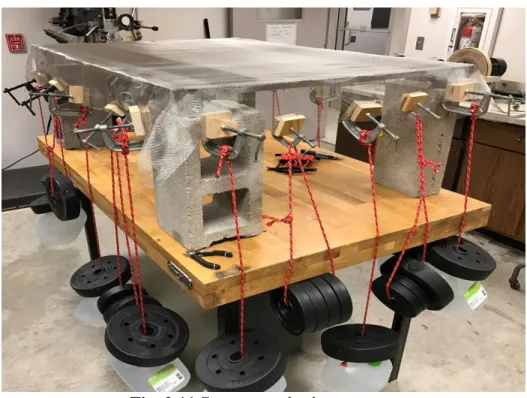
The settling chamber was manufactured by the UIUC Aerospace Engineering Machine Shop and myself. The walls of the settling chamber were made of 1/4 inch thick aluminum 6061 flat bar. Each piece was machined into a panel that served as a track system for the screen and honeycomb frame to be slid into. The slots machined into each panel are presented in Fig. 2.10, with the freestream direction from left to right. Each panel was connected to the neighboring panel with 3 inch x 1 inch x 1/8 in thick aluminum C-channels. The screen frames were made out of 1 inch by 1/8 inch thick aluminum flat bar and 1/8 inch thick aluminum L stock with 1 inch legs. Each screen was laid over the L stock frame and then the flat bar was bolted down on top using counter sunk head 10-24 screws and nuts. Each screen was pulled taut using a custom tensioning system presented in Fig. 2.11. The tensioning system consisted of barbell weights and gallon water jugs hung with ropes that were attached to the screens with C-clamps. The C-clamps were synched down to the screen with wood blocks placed on either side of the screen. Once the screens were tensioned from the pulling force of the weights, the aluminum flat bar was attached to hold the screen in place without losing tension.

(36)

23

Fig. 2.11 Screen tensioning system.

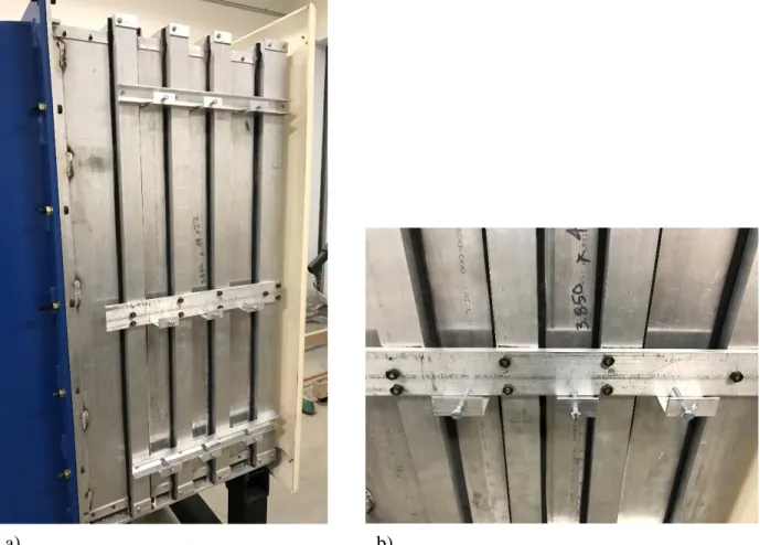
The L-stock flat bar frame, presented in Fig. 2.12 a) and b), was designed to slide into the wall panels so that the inside face of the panel and L-stock were flush. Due to manufacturing tolerances the transition between panel and L-stock were not perfectly flush on some walls. However, a previous study on screen frame steps showed that turbulence intensities compared closely to frames with steps as frames that are flush.10 Also, the mass flow rate for the blower system will be slightly higher due to pressure loss from the step, but flow angularity will be virtually unaffected by the step.10 The low velocity in the settling chamber made it a very forgiving section of the wind tunnel in terms of aerodynamic performance. The honeycomb frame was manufactured out of 1/8 inch aluminum L-stock, one side with 1 inch legs and on side with 1 and 1.5 inch legs. The L-stock was bolted together facing opposite directions so that the length of the frame was 2.5 inches and the 1 inch L-stock legs were facing outward, presented in Fig. 2.13 a) and b). The frame was then attached around the honeycomb core one side at a time in order to ensure a tight, pressed fit that hold the honeycomb in place during tunnel operation.

(37)

24

Fig. 2.12 a) Turbulence screen assembly; b) screen L-stock and flatbar frame.

Fig. 2.13 a) Honeycomb assembly; b) honeycomb L-stock frame.

a) b)

(38)

25

Each panel group consisted of four walls connected at the corners with 1/8 inch thick aluminum 90 degree L-stock with 1 inch legs. The angles were fastened to the outside of the panels with 8-32 bolts as presented in Fig. 2.14. Each panel group, one between the nozzle and the last screen, one between each screen, and one between the first screen and the honeycomb were attached together with the C-channel. The C-channels were welded to the panels one by one, with 1/16 inch shims (2 on each side) placed between the screen frame and the next panel to ensure that the screens could slide in and out of the settling chamber frame. The flange that attached the settling chamber to the inlet was manufactured out of 3/8 inch aluminum flat bar with 9/16 inch holes placed in the same pattern as the nozzle flange. The flange was welded to the settling chamber with 1/4 inch thick aluminum L-stock with 1 inch legs. To seal in the settling chamber, RTV silicone gasket was applied to all of the creases and sections that were not welded. The entrance to the settling chamber was equipped with 4 inch diameter PVC pipe to help guide the flow into the honeycomb of the window tunnel, presented in Fig. 2.15 a) and b).

(39)

26

Fig. 2.15 a) PVC entrance; b) PVC entrance attached to settling chamber.

The screens and honeycombs must be serviced annually (or more frequently) to remove dust and other particles preventing clean air passage. This build up of dust can cause a significant pressure loss and reduce the performance of the wind tunnel. For these reasons, an access door was made on one of the walls of the settling chamber in order remove the screens and honeycomb. The access door was manufactured out of aluminum C-channel and flat bar, presented in Fig. 2.16 a). Each C-channel covers the hole that the screens and honeycomb slide into. To seal in the access panel, foam weather stripping was placed on the outside face of each of the panels. The access door was pressed into the foam via 1/4”-20 bolts at nine locations to ensure an airtight seal, presented in Fig. 2.16 b).

(40)

27

Fig. 2.16 a) Settling chamber access door; b) bolting bracket to seal access door.

2.4 Diffuser

The diffuser section of the wind tunnel decelerated the flow through area expansion, allowing a gradual pressure recovery close to atmospheric conditions. In this tunnel, the exit diffuser was located aft of the test section, before the air enters the blower system. While often overlooked, an efficient diffuser design is one of the most important aspects of the development of a transonic wind tunnel. According to Goethert1, in an example continuous transonic wind tunnel, the pressure loss distribution in the diffuser constituted 41% of the total losses of the entire tunnel. If a diffuser is too short, the flow will separate from the wall, producing large pressure losses. Conversely, if a diffuser is too long and with gradual area change, the losses due to viscous effects become significant, leading to large pressure losses.

(41)

28

2.4.1 Diffuser Expansion Angle

The flow through the diffuser depends solely on its geometry and can be defined by its wall expansion angle, area ratio, cross-sectional shape, and wall contour.19_{Three of these parameters}

were fixed due to the test section size, blower entrance size and shape, and the manufactures ability to fabricate the wall contour. The only parameter that could be adjusted was the diffuser expansion angle. The diffuser was configured to transition from a 6 inch x 9 inch rectangular test section to a 23 inch diameter circle at the entrance of the blower. The expansion half-angle was calculated to identify the angle between the edges of the test section plane to the edges of the blower entrance plane. This angle is taken from the plane perpendicular to the planes of the test section and blower entrance. The 3D model of the diffuser is presented in Fig. 2.17 and shows the expansion half-angle. The total expansion angle was found by adding the two half angles on opposite sides together. This total angle can also be called the “equivalent cone angle,” defined as the included angle of a circular cone having the same inlet area, outlet area and length as the given diffuser.19 The equivalent cone angle should be between 5 degrees (for best flow steadiness) and 10 degrees (for best pressure recovery).19 Typically, diffusers are designed to have a maximum expansion angle (combined across both walls) of 7.5 degrees.20 This angle was chosen for the benefits of both flow steadiness and pressure recovery. While a very long diffuser (small angle) provides a deceleration with little chance of flow separation, the pressure losses and power requirements do to the large length can be costly. In contrast, while a short wide-angle diffuser (large angle) provides great pressure recovery, the change of flow separation and unsteadiness was high. Due to the rectangular test section, the expansion angle could not be the same for the transition from the top and bottom to the blower entrance as is from the sides. Therefore, an expansion half-angle of 3.75 degrees was used for the sides and 3.09 degrees for the top and bottom (calculated by taking the arc tangent of the vertical difference between the top of the test section to the top of the blower entrance and the total length of the diffuser). The expansion angle defined the length of the diffuser, the final design was 129.685 inches.

(42)

29

Fig. 2.17 a) Diffuser side view; b) diffuser isometric view.

The velocity at the exit of the diffuser was calculated from the area of the exit plane and mass flow rate for operating conditions. Dividing the mass flow rate by the area and converting units gives a velocity of 125 ft/s and a Mach number of M=0.11. Therefore, it can be stated that the diffuser decelerates the flow to an adequate velocity for the blower system volumetric flow rate of 21,500 CFM.

2.4.2 Diffuser Material and Manufacturing

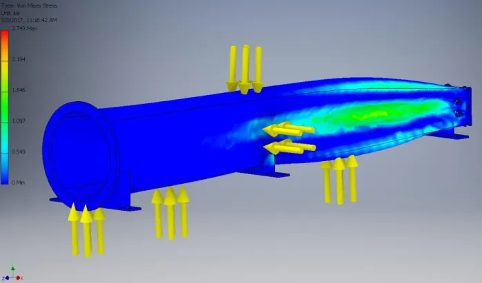
The diffuser and nozzle were manufactured from 3/8 inch thick steel. A finite element analysis (FEA), presented in Fig. 2.18 and Fig. 2.19, was performed based on the pressure differential in the diffuser and the ambient laboratory conditions. The static pressure inside the wind tunnel will be lower than the atmospheric pressure outside the tunnel due to the increase in dynamic pressure inside the tunnel. The FEA was performed for the largest pressure differential when the test section Mach number is at the maximum of M=0.8. Since the outside of the tunnel

a)

(43)

30

was at atmospheric pressure, the pressure differential was equal to the dynamic pressure inside the tunnel. This was calculated using,

(2.12)

where 𝒒 is the dynamic pressure, 𝝆 is the air density at sea level, 𝑴 is the test section Mach number, and 𝒂 is the speed of sound at sea level. The dynamic pressure was calculated to be 6.6 psi. Although the pressure differential would decrease down the length of the diffuser due to the increase in pressure caused by area change, the largest pressure was applied over the entire diffuser for a conservative estimate. Two materials, steel and aluminum 6061, were analyzed at both 1/4 inch and 3/8 inch thickness. When put through the FEA simulation, the diffuser was constrained on both the upstream and downstream flange faces, as well as the flange faces on the bottom that connected to the structure assembly. To be conservative, a pressure of 7 psi was applied to the outside surface in case the Mach number ever went above M=0.8 in the diffuser and/or nozzle. Also, this conservative estimate took the pressure loss from the settling chamber into account, resulting in a large pressure differential. Since the pressure was greater on the outside of the tunnel, the stress and displacement would be induced inward (pressure moves from high to low), as presented in Fig. 2.18 and Fig. 2.19 by arrows. In Fig. 2.18, the Von Mises stress is shown, with the largest stress for 3/8 inch steel reaching 2743 psi, well below the yield strength of steel, 36260 psi.21 In Fig. 2.19, the largest displacement for 3/8 inch steel was in the X direction of 0.00467 inches. When the simulation was ran for 1/4 inch thickness, the stress of both aluminum and steel was below the yield strength. However, the displacement calculated was significantly larger and could result in significant vibrations, especially in the presence of shocks. For this reason, the thickness of 3/8 inches was selected for both the diffuser and nozzle. The cost of manufacturing the parts out of steel was significantly less expensive than that of aluminum 6061, therefore both were made of steel.

𝑞 =1

2∗ 𝜌 ∗ (𝑀 ∗ 𝑎) 2

(44)

31

Fig. 2.18 Diffuser FEA: Von Mises stress.

(45)

32

The nozzle and diffuser were manufactured by Fox Valley Metal Tech by bending and shaping the parts to the specified dimensions. The parts were welded together after each panel was formed. As an added measure of safety, a sheet of metal twisted-wire fencing was installed between the downstream end of the diffuser and the blower entrance flanges. The hexagonal openings were 1 in (height) by 1.5 in (width) with a wire diameter of 0.035 inches. The fencing will stop any large objects that may come down the tunnel from hitting and possibly damaging the blades of the fan. The horizontal flanges were 1/2 inch thick and connected to the structural assembly with 1/2” -13 socket head bolts, washers, and nuts. The circular flange that connected the diffuser to the blower was attached with 1/2”-13 socket head bolts, washers, and nuts.

2.5 Test Section

The test section of a transonic wind tunnel is where the majority of design and operating challenges occur. Due to the characteristics of transonic flow, careful design of the test section is pertinent to avoid shock reflection and/or local flow choking. The design of the components that will be implemented to address these challenges will be discussed in detail in the following section. These components included open-area walls, suction plenums, diffuser entrance flaps, choke vanes, test section windows, and the airfoil mounting apparatus. The test section model is presented in Fig. 2.20.

(46)

33

2.5.1 Open-area Walls

In order to prevent shock reflections and shocks in the test section due to choking, open-area walls were implemented. These open-open-area walls were configured on the top and bottom walls of the test section that allow air to flow into a suction plenum, which is discussed in section 2.5.2. It was identified in the 1950’s that shock reflections could be canceled in a closed-wall wind tunnel with the use of longitudinal slots on the test-section walls.22 It was later shown that wall-induced effects can be mitigated even more significantly with the use of porous wind tunnel walls.23 Mitigation of shock reflections and test section choking was accomplished by matching the plenum pressure to that within the test section, which simulates free-flight conditions with no walls.

Perforated or porous walls were selected instead of slotted walls because the Mach number distribution has been observed to be more stable. The results from experiments performed in wind tunnels with both porous and slotted walls are presented in Fig. 2.21 a) and b). The Mach number distribution was more stable for all open-area ratios with the perforated walls when compared to the slotted walls. For both the perforated and slotted test sections, the Mach number distribution across the beginning stages of the test section is not very sensitive to the slot or porous shape or open-area ratio.1 It is only at the downstream end of the test section where local disturbances in Mach number distribution frequently occur, and these can be controlled with a suction chamber.1 The downstream end, especially when an airfoil is present in the test section, is where the porous walls have the advantage due to the more evenly distributed open-area.

(47)

34

Fig. 2.21 a) Mach number distribution with perforated walls;24_{b) Mach number distribution} with slotted walls.25

Typical open-area ratios for perforated walls range from 5% to 33% and are more efficient if the holes are inclined towards the streamwise direction.1 The open-area ratio is the amount of area that air is allowed to freely pass through the wall to that of the total area of the wall. Plate thickness and diameter of the pores are important to avoid a diffuser effect.1 The diffuser effect is an increase in pressure as air passes through the wall because the thickness of the plate was too large relative to the diameter of the pores, creating a long channel for the air to travel through. The open-area ratio, plate thickness to diameter ratio, and hole inclination were selected based on experimental results shown in Fig. 2.22 and Fig. 2.23. As shown in Fig. 2.22 the open-area ratio can be reduced to 6% from 22.5% with the inclination of holes at 60 degrees in the orientation presented in Fig. 2.24. From the plots in Fig. 2.22 and Fig. 2.23, the mass flow (X axis) required to achieve the minimum pressure differential (Y axis) between the test section and suction plenum was lowest for a 6% open-are ratio, 60 degree inclination, and hole diameter to wall thickness ratio of 1. The test results for 6% open-area ratio walls with 60 degree inclined holes indicate consistent nearly-linear characteristics when the hole diameters are equal to or twice as large as the wall thickness.1_{Therefore, the lower the mass flow rate, the less power is required to produce the}

adequate suction. The pressure drop across the thin plate is proportional to the angle of the wall

(48)

35

and the incoming flow.1 With an inclination of 60 degrees, this pressure drop can be reduced, and is much smaller relative to the pressure change caused by the diffuser effect with thick walls. The inclination also prevents the air in the suction plenums to come back into the test section.

Fig. 2.22 Comparison of perforated walls with straight holes and inclined holes at different open-area ratios.1

Fig. 2.23 Cross-flow characteristics of perforated walls with 60 degree inclined holes for various ratios of hole diameter to wall thickness, open-area ratio 6% at M=0.90.1

(49)

36

Fig. 2.24 Hole inclination orientation.1

The final dimensions of the plates are 15 inches (length) by 6.5 inches (width) by 1/4 in (thickness), presented in Fig. 2.25. The holes were drilled at an incline of 60 degrees with a diameter of 1/4 inches. The holes were space evenly across the surface of the plate with an open-area ratio of 6%. The plates were attached to the vertical test section walls with socket head 3-48 screws, with through holes provided for the screws of the suction plenums. The left and right sides of the plates overlay on the vertical test section walls by 1/4 inches to hold the width of the test section to 6 inches. The upstream section of the plates had a 1/4 inch (length) by 1/16 inch (thickness) lip that connects to the upstream top and bottom walls of the test section. This resulted in a solid walled test section for the first 3.25 inches to let the airflow stabilize before the suction through the pores began. The plates run to the end of the test section, therefore it had 3.25 inches of solid walls and 14.75 inches of porous walls for a total test section length of 18 inches. A slot was placed on the top porous plate, presented in Fig. 2.26, to give passage for a PIV laser sheet, discussed in detail in section 2.6.2. The top plate is equipped with a static pressure port for both sides of the plate to calculate the pressure differential between the plenum and the test section, discussed in detail in section 2.6.3. This pressure differential is controlled by the suction control flaps, discussed in detail in section 2.5.3.

(50)

37

Fig. 2.25 Porous plate model.