Efficient algorithms for distributed learning, optimization and belief systems over networks

(1)

c

(2)

EFFICIENT ALGORITHMS FOR DISTRIBUTED LEARNING, OPTIMIZATION AND BELIEF SYSTEMS OVER NETWORKS

BY

C´ESAR A. URIBE MENESES

DISSERTATION

Submitted in partial fulfillment of the requirements

for the degree of Doctor of Philosophy in Electrical and Computer Engineering in the Graduate College of the

University of Illinois at Urbana-Champaign, 2018

Urbana, Illinois Doctoral Committee:

Professor Tamer Ba¸sar, Chair

Professor Angelia Nedi´c, Director of Research

Assistant Professor Alex Olshevsky, Co-Director of Research Professor Rayadurgam Srikant

(3)

ABSTRACT

A distributed system is composed of independent agents, machines, processing units, etc., where interactions between them are usually constrained by a network structure. In contrast to centralized approaches where all information and computation resources are available at a single location, agents on a distributed system can only use locally available information. The particular flexibilities induced by a distributed structure make it suitable for large-scale problems involving large quantities of data. Specifically, the increasing amount of data generated by inherently distributed systems such as social media, sensor networks, and cloud-based databases has brought considerable attention to distributed data processing techniques on several fronts of applied and theoretical machine learning, robotics, resource allocation, among many others. As a result, much effort has been put into the design of efficient distributed algorithms that take into account the communication constraints and make coordinated decisions in a fully distributed manner.

In this dissertation, we focus on the principled design and analysis of distributed algorithms for optimization, learning and belief systems over networks. Particularly, we are interested in the non-asymptotic analysis of various distributed algorithms and the explicit influence of the topology of the network they ought to be solved over.

Initially, we analyze a recently proposed model for opinion dynamics in belief systems with logic constraints. Opinion dynamics are a natural model for a distributed system and serve as an introductory topic for the further study of learning and optimization over networks. We assume there is an underlying structure of social relations, represented by a social network, and people in this social group interact by exchanging opinions about a number of truth statements. We analyze, from a graph-theoretic point of view, this belief system when a set of logic constraints relate the opinions on the several topics being discussed. We provide novel graph-theoretic conditions for convergence, explicit estimates of the convergence rate and the limiting value of the opinions for all agents in the network in terms of the topology of the social structure of the agents and the topology induced by the set of logic constraints. We derive explicit dependencies for a number of well-known graph topologies.

(4)

where a group of agents interact over a network and seek to estimate a joint parameter that best explains a set of network-wide observations using the local information only. Again, we assume there is an underlying network that defines the communication constraints between the agents and derive explicit, non-asymptotic, and geometric convergence rates for the concentration of beliefs on the optimal parameter. For the case of having a finite number of hypotheses, we propose distributed learning algorithms for time-varying undirected graphs, time-varying directed graphs and a new acceleration scheme for fixed undirected graphs. For each of the network structures, we present explicit dependencies for the worst case network topology. Furthermore, we extend these belief concentration results to hypotheses sets being a compact subset of the real numbers, for a simplified static undirected network assumption. Moreover, we present a generic distributed parameter estimation algorithm for observational models belonging to the exponential family of distributions. We further extend the distributed mean estimation from Gaussian observations to time-varying directed networks.

The graph-theoretical analysis of belief systems with logic constraints and the distributed learning for cooperative inference are specific instances of convex optimization problems where the objective function is decomposable as the sum of convex functions. Particularly, these problems assume each of the summands is held by a node on a graph and agents are oblivious to the network topology. As a final object of interest, we study the optimality of first-order distributed optimization algorithms for general convex optimization problems. We focus on understanding the fundamental limits induced by the distributed networked struc-ture of the problem and how it compares with the hypothetical case of having centralized computations available. We show that for large classes of convex optimization problems, we can design optimal algorithms that can be executed over a network in a distributed manner while matching lower complexity bounds of their centralized counterparts with an additional iteration cost that depends on the network structure. We design optimal distributed algo-rithms for various convexity and smoothness properties that can be executed over arbitrary fixed, connected and undirected graphs. Furthermore, we explore the application of these distributed algorithms to the problem of distributed computation of Wasserstein barycenters of finite distributions.

Finally, we discuss some future directions of research for the design and analysis of dis-tributed algorithms, both from theoretical and applied perspectives.

(5)

(6)

ACKNOWLEDGMENTS

Every thesis acknowledgment starts with something like: “This wouldn’t have been possible without Prof...” This one will not be any different, not to keep the clich´e alive, but because nothing could be closer to reality. I cannot imagine having better advisers than Prof. Angelia Nedi´c and Prof. Alex Olshevsky. They provided me with the unique opportunity to have the intellectual freedom to explore several research problems. Moreover, they provided me constant and uninterrupted guidance and were extremely generous with their patience. Their advice was invaluable at every scale, from a missing comma in a draft and a loop-hole in a proof to the big picture on relevant open problems. Most importantly I am grateful for their trust. This is the first necessary condition to enjoy and complete any doctoral program.

Of course, the second necessary condition for a successful Ph.D. is to have constant support from the loved ones. Mamá, Papá, Angelica, Mary, muchas gracias por confiar en m´ı y darme todo el apoyo que necesité. Ustedes son la esperanza que mantiene mi motivación siempre alta. Nunca los saqué de mi mente. Sandra, there are no words to express the infinite value you have brought to my life. Your company is calm in the hardest times.

The third necessary condition is to have a great committee for the defense. My gratitude goes to Prof. Tamer Ba¸sar for allowing me to take part in his group meetings, being attentive to the development of my dissertation and kindly agreeing to be the chair of my defense. No other course influenced more the contents of this dissertation than Statistical Learning Theory by Prof. Maxim Raginsky. His unlimited knowledge of the literature both in English and Russian was always readily available. Finally, I am thankful to Prof. Srikant; he always has the precise personal and professional advice that can only come from experience. His kind invitation to be his TA and attend his group meetings gave me a number of new experiences that only strengthened my professional profile.

The fourth necessary condition is to have unbelievably talented colleagues, and CSL is the place to find them. Being surrounded by extremely smart people is humbling and puts things in perspective. Some people say one is the average of the five people one spends the most time with. CSL always brought this average higher. Many thanks, Philip, Thinh, Amir, Jaeho, James, Prof. Rasoul Etesami, Prof. Behrouz Touri, Dr. Soomin Lee, Dr. Wei Shi, and all the

(7)

ones I am missing. I also thank Dr. Hoi-To Wai for his friendship and welcoming attitude during my time in Arizona. Finally, I am most thankful to Prof. Alexander Gasnikov. His illuminating discussions and unparalleled understanding of mathematical programming were fundamental for the realization of the later parts of this dissertation.

Being away from home is never easy. However, no matter how cold Chambana got, the Colombian crew made me always feel like I was in the tropics. During these years, I met great Colombian and Latin-American scientists. I was always amazed at how much talent our region is able to produce in spite of all the adverse circumstances. Thanks a lot Ian & Angela, Jorge & Monica, Wladimir & Monika, Santiago & Ana, Agustin & Fernanda, Camila & Pedro, Ximena & Mauricio, Ian & Lina, Catalina & Fabian, Eliana, Daniel, Felipe, Santiago & Mariam, Rafa & Catalina, Liz, JJ, Rocio, and all others I’m unconsciously forgetting to keep this dissertation finite.

Life in Chambana would have been much sadder without volleyball. Here is where I would always be thankful for the Rec Volleyball Club. Being able to play every Wednesday allowed me to meet great players, but foremost, great people who made my winter days warm. Especially, I want to do a shout-out to the No-Name team. Thank you Pavel, Dima, Evelyn, Eric and Drake for being the most amazing undefeated team in the whole of Urbana-Champaign. It was an honor to play with you guys.

(8)

LIST OF TABLES

1.1 Maximum expected convergence time for a random walk on networks with

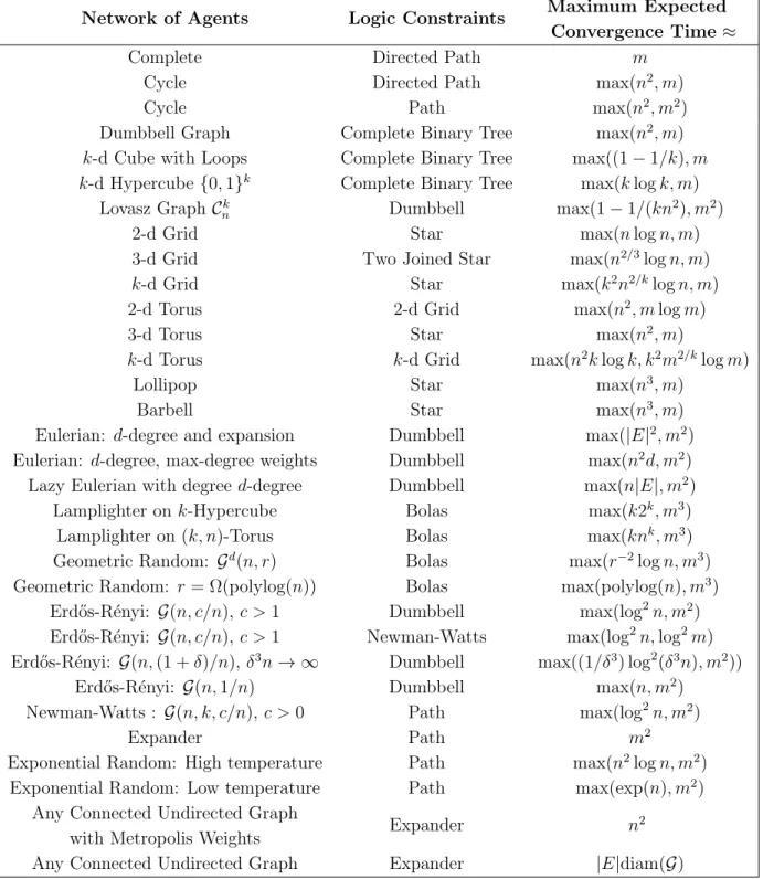
n nodes. . . 17 2.1 Maximum Expected Convergence Time for the belief system with Logic

Constraints for different networks of Agents withn nodes and networks of

truth statements with m nodes. . . 41 2.2 Datasets of Large-Scale Networks. . . 49 2.3 Size of the highly influential cliques and the number of iterations required

for them to drive the fast mixing of a random walk on the three examples

of large scale graphs. . . 51 5.1 Iteration Complexity of Distributed Optimization Algorithms. . . 137 5.2 A summary of algorithmic performance. . . 149

(11)

LIST OF FIGURES

1.1 The object of study of this thesis . . . 3

1.2 Examples of common graphs. . . 10

2.1 A belief system with 4 agents and 3 truth statements . . . 25

2.2 A belief system with agents on a cycle graph and logic constraints on a path graph. . . 27

2.3 The influence of the logic constraints in the resulting aggregated belief system. 28 2.4 Two examples of graph product between a complete graph/cycle graph with 5 nodes and a path graph of 4 logical belief constraints. . . 29

2.5 Open and closed strongly connected components of a graph. . . 30

2.6 Hitting and absorbing time of a random walk . . . 33

2.7 Convergence time for a belief system with an undirected cycle as a social network and a directed path as a network for the logic constraints. . . 39

2.8 Examples of random graphs. . . 42

2.9 Convergence time or various belief systems. . . 43

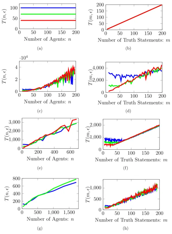
2.10 Convergence time for different examples of networks of agents and network of truth statements in a belief system. . . 44

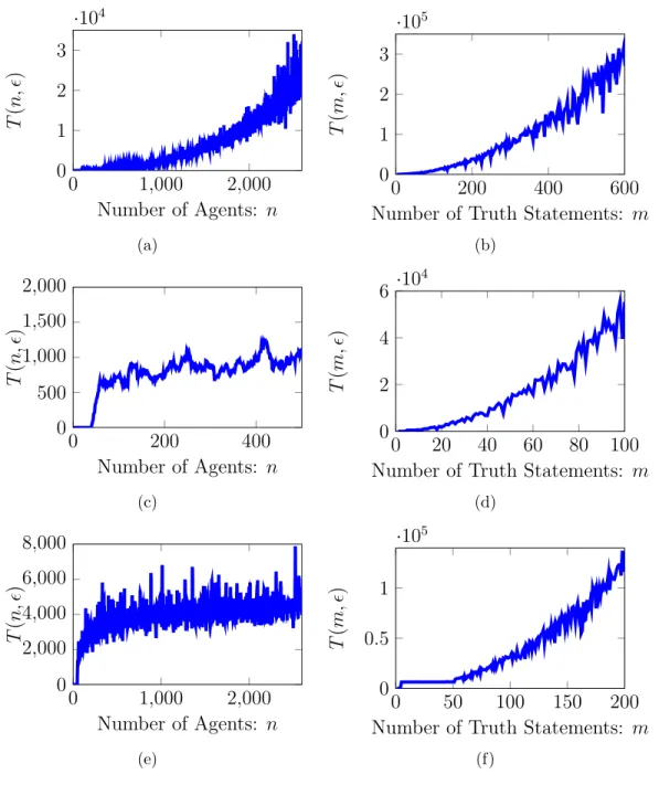
2.11 Convergence time dependency for random graphs. . . 45

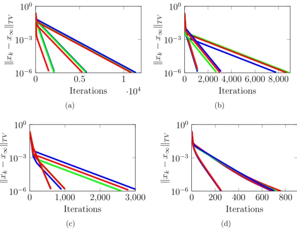
2.12 Exponentially Fast Convergence of the Belief System. . . 46

2.13 Geometric convergence of the Belief system with random networks of agents. 47 2.14 Large-Scale Complex Networks from the Stanford Network Analysis Project (SNAP). . . 50

2.15 Cumulative Social Power of the agents. . . 52

2.16 Convergence Time of Belief System with Large-Scale Complex Networks. . . 53

2.17 Total variation distance between the beliefs and its limiting value as the number of iteration increases. . . 54

3.1 A network of 4 agents. . . 61

3.2 Geometric interpretation of the learning objective. . . 62

3.3 Conflicting social groups interacting. . . 69

3.4 Empirical mean over 50 Monte Carlo runs of the number of iterations required forµi k(θ)< for all agents on θ /∈Θ∗. . . 89

3.5 Distributed source localization example. . . 93

3.6 Source localization on a grid with 3 agents and 9 hypotheses. . . 94

(12)

3.8 Network of Agents and Belief of one agent on the optimal hypothesis. . . 96

3.9 Network of Normal, Failed and No-Sensor Agents and Belief of one agent on the optimal hypothesis. . . 96

4.1 Creating a covering for a ball _Br . . . 99

4.2 Creating a covering for a set_Br. . . 104

4.3 Hellinger distance of the density pθ to the optimal density pθ∗. . . 105

4.4 Distributed Estimation of a Network-side Mean from Gaussian Observations. 122 4.5 Distributed Estimation of a Network-side Variance from Gaussian Observations.123 4.6 Distributed Estimation of a Network-side Mean and Variance from Gaus-sian Observations. . . 124

4.7 Distributed Estimation of a Network-side Parameter from Bernoulli Ob-servations. . . 125

4.8 Distributed Estimation of a Network-side Parameter from Poisson Observations.126 4.9 Distributed Estimation of a Network-side Parameter from Exponential Ob-servations. . . 127

4.10 Distributed Gaussian Learning on a Grid Graph. . . 133

4.11 Distributed Gaussian Learning on a Path Graph. . . 133

4.12 Distributed Gaussian Learning on a Path Graph and heterogeneous variances. 134 4.13 A particularly bad graph. . . 134

4.14 Distributed Gaussian Learning on a particularly bad graph. . . 135

5.1 Two examples of networks of agents. . . 152

5.2 Distance to optimality and consensus, and network scalability for a strongly convex and smooth problem. . . 155

5.3 Distance to optimality and consensus, and network scalability for a strongly convex andM-Lipschitz problem over a cycle graph. . . 156

5.4 Distance to optimality and consensus for Erd˝os-R´enyi random graph (right) and cycle graph for smooth functions. . . 157

5.5 Distance to optimality and consensus for Erd˝os-R´enyi random graph (right) and cycle graph for smooth problems and various values of the regulariza-tion parameter. . . 157

5.6 Samples of the digit 7 from the MNIST dataset and comparison of their Euclidean and Wasserstein Barycenters. . . 158

5.7 Erd˝os-R´enyi random graph where each agent privately holds a sample of the digit 7 from the MNIST dataset. . . 159

5.8 Optimality and Scalability of Algorithm (5) for various graphs. . . 168

5.9 Local Wasserstein Barycenter of the digits of the MNIST dataset for a subset of 3 agents. . . 170

(13)

LIST OF SYMBOLS

x∈Rd _{A column vector in} _Rd

1d A column vector of dimension d with all entries equal to 1 G(V, E) A static undirected graph with node set V and edge set E a.s. Almost surely, with probability 1

kx_k or_kx_k2 Euclidean norm of vector x

i.i.d. Independent and identically distributed hx, y_i Inner product of two vectors x and y

·k or·t Subindices k and t are usually reserved to iteration or time indices

·i _or_·j _Superindices _i _and _j _{are usually reserved to indicated values at the nodes} |S_| The cardinality of a set S

Sc _{The complement of a set} _S

Akf:ki The cumulative product Akf:ki =Akf ·Aki+1Aki for all kf ≥ki ≥0

di _or _deg(i) _{The degree of a node} _i

E∗ The dual space of the finite-dimensional vector spaceE

[A]ij oraij The entry of the matrix A at the i-th row and the j-th column

E[·] The expectation of an event

S1(n) The finite probability simplex such thatS1(n) ={p∈Rn+|pT1= 1}

h2_{(P, Q)} _{The Hellinger distance between distributions} _P _and _Q

[x]i orxi The i-th entry of a vector x Id The identity matrix of size d

(14)

ker(W) The kernel of matrix W

A_⊗B The Kronecker product between objects A and B

DKL(PkQ) The Kullback-Leibler divergence between distributions P and Q λmax(W) The largest eigenvalue of a matrixW

dmax and dmin The maximum and minimum degree of a graph

σmax(W) The maximum eigenvalue of the matrix WTW, i.e., λmax(WTW)

kA_kE→H The norm of a linear operator A:E →H such that kAkE→H = maxx∈E,u∈H∗{hu, Axi | kxk_E = 1,kuk_H∗ = 1} ⊥ The orthogonality symbol between two vectors

kx_kp The p-norm of vectorx d(G) The period of a graph G

P[_·] The probability of an event

X ∼P The random variable X is distributed according to P λ2(W) The second largest eigenvalue of a matrix W

Rd _{The set of} _{d-dimensional vectors with components in} _R Ni

k The set of neighbors of agent i at time k

R+ The set of nonnegative real numbers

R The set of real numbers

λ+_min(W) The smallest positive eigenvalue of a matrix W

σ_min+ (W) The smallest positive eigenvalue of the matrix WT_W_{, i.e.,} _λ+

min(WTW)

span(W) The span of matrix W x0 _or_xT _{The transpose of a vector} _x

(15)

CHAPTER 1 INTRODUCTION

Large numbers of interconnected components add to the complexity of engineering systems. Developing models and tools for the analysis of such distributed systems is necessary, not only from the engineering point of view but for effective decision-making and policy design. For example, the control of autonomous vehicles for exploration, rescue, and surveillance depends on the coordination abilities of fleets of robots; each robot should make decisions based on local information and limited communications. Power networks (e.g., the electric grid) need several generating and consuming stations to coordinate offer and demand to improve efficiency. In traffic control, the goal is to avoid jams distributively and to increase traffic flow based on limited infrastructure (e.g., roads). Economic systems need modeling, estimation, and control of markets at the micro and macroeconomic scales. Market dynam-ics depend on several agents influencing the system, each of which might have conflicting goals. In telecommunication networks, several stations need to communicate over non-perfect channels to optimize information transmission. The control of industrial processes requires communication and coordination between different parts of the process in hazardous envi-ronments. The modeling and control of ecological systems requires the analysis of several actors interacting with each other, subject to changing environments.

The increasing amount of data generated by recent applications of distributed systems such as social media, sensor networks, and cloud-based databases has brought considerable attention to distributed data processing, in particular the design of distributed algorithms that take into account the communication constraints and make coordinated decisions in a distributed manner [1, 2, 3, 4, 5, 6, 7, 8, 9, 10, 11]. In a distributed system, interactions between agents are usually constrained by the network structure and agents can only use lo-cally available information. This contrasts with centralized approaches where all information and computation resources are available at a single location [12, 13, 14, 15].

Traditional approaches for the design of distributed inference algorithms, for inherently distributed systems, assume a fusion center exists. The fusion center gathers all the in-formation and makes centralized decisions [12, 13, 14, 15]. Nonetheless, communication constraints, limited memory and lack of physical accessibility to certain measurements

(16)

hin-der this task. Therefore, it is necessary to develop algorithmic protocols that take into account such constraints and use only locally available information.

The adoption of distributed optimization algorithms on several fronts of applied and the-oretical machine learning, robotics, and resource allocation has increased the attention on such methods in recent years [16, 17, 18, 19, 20]. The particular flexibilities induced by the distributed setup make them suitable for large-scale learning problems involving large quantities of data [21, 22, 23, 24, 25]. Although many results on these themes have appeared in recent years, the study of distributed decision-making and computation traces back to classic papers from the 70s and 80s [5, 6, 7, 8, 9, 10, 11].

In [26] the authors defined society as “wise” if the influence of the most influential agents vanishes with the size of the network. This assumes there exists some balancedness in the network in terms of the agents’ centrality. Knowledge about the topology of the network can be used to design algorithms that take the agents’ connectivity into account, but this introduces additional information requirements and limits the ad-hoc nature of a distributed solution. Specifically, in evolving networks the connectivity of the agents’ changes with time and thus so does their influence, introducing variability in the group confidence.

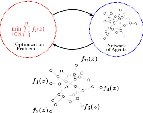
The object of study of this dissertation is twofold: on the one hand we have a convex optimization problem Pm_i₌₁fi(z) assumed to be the sum of a finite number n of convex functions, and on the other hand we have a network, modeled as a graph G(V, E), with |V_| = n nodes and a set of edges E between them that represent their ability to share information, see Fig. 1.1. The main property of this object is the assumption that each node i in the network has access to a single fi(z) only. Nonetheless, one seeks to solve the network-wide optimization problem by local interactions constrained by the network edges. Now that we have defined the main focus of this theses we can describe the specific problems we are interested in. We study four specific problems:

1. Graph-theoretic analysis of belief systems with logic constraints. min x∈Rn n X i=1 n X j=1 aijkxi−xjk2 ∀i∈V.

2. Distributed learning with finite hypotheses sets. min θ∈Θ n X i=1 DKL(PikPθi) Θ is finite.

(17)

min

z_∈R n

P

i=1

f

_i

(

z

)

Optimization

)

Figure 1.1: The object of study of this dissertation. 3. Distributed learning on compact hypotheses sets.

min θ∈Θ⊂Rd n X i=1 DKL(PikPθi) Θ is compact.

4. Optimal algorithms for distributed optimization. min z∈R m X i=1 fi(z), such that

(a) Each fi is strongly convex and smooth. (b) Each fi is strongly convex.

(c) Each fi is smooth and convex. (d) Each fi is convex.

(18)

1.1 Motivation and Past Work

In this section, we introduce each of the problems studied in this dissertation and motivate the open problems for each case. We provide some classic references and guide the reader towards a more comprehensive literature review.

1.1.1 Opinion Dynamics in Belief Systems with Logic Constraints

The analysis and modeling of opinion dynamics spans several decades of interdisciplinary research [27, 28, 29, 30, 31, 32, 33, 34, 35]. Belief systems are modeled as a process where agents continuously update their beliefs by repeated interactions where opinions are ex-changed over some social structure (e.g., social network) [10, 36]. New opinions are formed by aggregating operations weighted by the relative importance assigned by an individual to others. This simple characterization has provided tools for analyzing the long-term behav-iors using systems theory. Nevertheless, the characterization has been shown insufficient to explain the existence of shared beliefs in a population [37].

Opinion formation cannot be described solely as an ideological deduction from a set of principles about the social world. Repeated social interactions and logic constraints on truth statements are consequential for the construction of belief systems as well. Recently proposed generalizations of opinion dynamic models integrate functional interdependencies among issues that coherently bound ideas and attitudes [38]. Mainly, logic constraints in belief systems provide a successful model for the evolution of opinions in both large-scale populations and small groups [37]. Logic constraints build upon the natural idea that be-lieving a specific statement is true may depend on the belief that other statements are true as well. Nonetheless, existing algebraic tools can be too complicated to use when facing large-scale and complex networks [38]. Understanding the role of the networks involved in the structural features of a belief system is of critical importance and can have direct implications for better decision-making and policy design [39, 40, 41, 42, 37].

We seek to provide graph-theoretic answers for a model of opinion dynamics of a belief system with logic constraints. Particularly, we are interested in showing how the belief system properties depend on the social network where agents interact and the set of logic constraints that relate beliefs on different truth statements. Moreover, we search for explicit dependencies for a variety of commonly used large-scale network models.

(19)

1.1.2 Distributed (Non-Bayesian) Learning over Networks

Numerous engineered and natural systems can be modeled as a group of agents interacting (e.g., people, robots, sensors). Distributed non-Bayesian learning studies groups of agents that try to “learn” a distribution (from a parametrized family) that best explains some observed data [1, 43, 44, 45, 46, 25, 47]. Specifically, agents seek to learn this parameter in a distributed manner where each agent accesses local information without the involvement of any centralized coordination.

One traditional problem in decision-making is that of parameter estimation. Given a set of noisy observations coming from a joint distribution, one would like to estimate a parameter or distribution that minimizes a certain loss function. For example, maximum a posteriori (MAP) or minimum least squared error (MLSE) estimators fit a parameter to some model of the observations. Both MAP and MLSE estimators require some form of Bayesian posterior computation based on models that explain the observations for a given parameter. Computation of such a posteriori distributions depends on having exact models about the likelihood of the corresponding observations. This is one of the main difficulties of using Bayesian approaches in a distributed setting. A fully Bayesian approach is not possible because full knowledge of the network structure, or of other agents’ likelihood models, may not be available [48, 49, 29].

In [29], the authors describe results on learning in social networks based on computing posterior distributions using Bayes’ rule. That is, given some assumed prior knowledge and new observations, an agent computes a posterior based on likelihood models, see [50]. Nevertheless, a fully Bayesian approach might not be possible because full knowledge of the network structure, or other agents’ likelihood models, need not be available [48, 49]. Other authors showed that non-Bayesian methods can be used in learning task as well [51, 1, 52, 43]. In this case, agents are assumed to be boundedly rational (i.e., fail to aggregate information in a fully Bayesian manner [26]). They repeatedly communicate with others and use naive approaches to aggregate information.

Several groundbreaking papers have described distributed methods to achieve global be-haviors by repeatedly aggregating local information without complete knowledge of the net-work [1, 2, 3, 4]. For example, in distributed hypothesis testing using belief propagation, convergence and its dependence on the communication structure were shown [3]. Later, extensions to finite capacity channels, packet losses, delayed communications, and tracking were developed [53, 54]. In [2], the authors proved convergence in probability, the asymptotic normality of the distributed estimation and provided conditions under which the distributed estimation is as good as a centralized one. Later in [1], the almost sure convergence of a

(20)

non-Bayesian rule based on the arithmetic mean was shown for fixed topology graphs. Ex-tensions to information heterogeneity and asymptotic convergence rates have been derived as well [52]. Following [1], other methods to aggregate Bayes estimates in a network have been explored. In [55], geometric means are used for fixed topologies as well. However, the consensus and learning steps are separated. The work in [56] extends the results of [1] to time-varying undirected graphs. In [43], local exponential rates of convergence for undi-rected gossip-like graphs are studied. The authors in [46, 45, 57, 56] proposed a non-Bayesian learning algorithm where a local Bayes’ update is followed by a consensus step. In [46], con-vergence result for fixed graphs is provided, and large deviation concon-vergence rates are given, proving the existence of a random time after which the beliefs will concentrate exponen-tially fast. In [45], similar probabilistic bounds for the rate of convergence are derived for fixed graphs, and comparisons with the centralized version of the learning rule are provided. Other variations of the non-Bayesian approach have been proposed for continuum set of hypotheses [58], weakly connected graphs [59], bisection search algorithms [60], transmission node failures [61, 62, 63] and time-varying graphs [64, 65, 66]. See [67, 68] for an extended literature review.

1.1.3 Optimal Convergence Rates in Distributed Optimization over

Networks

Early algorithms for distributed optimization, such as distributed subgradient methods, were shown successful for solving optimization problems in a distributed manner over networks [69, 70, 71, 72]. Nevertheless, these algorithms are particularly slow compared with their cen-tralized counterparts. Recently, distributed methods that achieve linear convergence rates for minimizing a sum of strongly convex and smooth (network) objective functions have been proposed. One can identify three main approaches to the study of distributed algorithms. In [73], a new method was proposed where it was shown that O((n2 ₊p_{L/µn) log}_ε−1₎

it-erations are required to find an ε solution to the optimization problem when the function is µ-strongly convex and L-smooth, and m is the number of nodes in the network. In [74], a new analysis technique for the convergence rate of distributed optimization algorithms via a semidefinite programming characterization was proposed. This approach provides an innovative procedure to numerically certify worst-case rates of a plethora of distributed algorithms, which can be useful to fine-tune parameters in existing algorithms based on feasibility conditions of a semidefinite program. In [75], a unifying approach was proposed, that recovers rate results from several existing algorithms such as those in [76, 77]. This

(21)

newly proposed general method is able to recover existing rates and achieves anεprecision in O(pL/(µλ2) logε−1) iterations, where λ2 is the second largest eigenvalue of the interaction

matrix. These results require some minimal information about the topology of the network and provide explicit statements about the dependency of the convergence rate on the prob-lem parameters. Specifically, polynomial scalability is shown with the network parameter for particular choices of small enough step-sizes, and even uncoordinated step-sizes are al-lowed [78]. One particular advantage of this approach is that it can handle time-varying and directed graphs. Nevertheless, optimal dependencies on the problem parameters and tight convergence rate bounds are far less understood. A third approach was recently introduced in [79], where the first optimal algorithm for distributed optimization problems was pro-posed. This new method achieves an ε precision in O(pL/µ(1 +τ /√γ) logε−1_{) iterations}

forµ-strongly convex andL-smooth problems, whereτ is the diameter of the network and γ is the normalized eigengap of the interaction matrix. Even though extra information about the topology of the network is required, the work in [79] provides a coherent understanding of the optimal convergence rates and its dependencies on the communication network.

One particular area of interest is the large-scale optimal transport problems. Optimal transport distances (also known as earth mover’s distances or Wasserstein distances) de-sign an optimal plan to move “mass” from one probability distribution to another. This problem can be traced back to the early work of Monge [80] and Kantorovich [81] and has been of constant interest for allowing natural formulations to the problems of comparing, interpolating, and measuring distances of functions [82]. On the other hand, computational optimal transport has gained popularity for its applications in learning theory [83], com-puter vision [84], comcom-puter graphics [85], statistical inference [86], information fusion [87], and its relative complexity advantages with respect to classical methods [88]. Particularly,

large-scale optimal transport has been of recent interest for the latest applications where large quantities of data are available and efficient algorithms are required [89, 90, 91]. Com-prehensive accounts of the optimal transport problem and its computational aspects can be found in [92, 93, 94, 82].

1.2 Dissertation Structure and Contributions

As indicated earlier, this dissertation is devoted to the study of the relation between op-timization problems in the form of a sum of convex functions and distributed networks. Moreover, we are particularly interested in the design of distributed algorithms that can be executed over a network where each node only requires local information and yet global

(22)

performance goals are achieved. For each of the studied problems and algorithms, we fo-cused on non-asymptotic performance analysis by looking into their efficiency and scalability concerning the structural properties of the problem and the topology of the network where the problem needs to be solved. Next, we provide a summary of the main contributions of this dissertation.

In Chapter 2, we study how the structural properties of the social network of agents and the set of logic constraints influence the dynamics of a belief system from a graph-theoretic point of view. We describe this influence for the convergence of beliefs, the expected convergence time and the stationary value of the belief system. Informally, we answer the following three questions with graph-theoretic conditions that are easily accessible for a number of commonly used topologies in large-scale complex networks: When does a belief system converge? How long does it take converge? What does it converge to?

In Chapter 3, we consider the problem of distributed learning, where a network of agents collectively aims to agree on a hypothesis that best explains a set of distributed observations of conditionally independent random processes. We focus on the case where the number of hypotheses is finite and propose a distributed algorithm and establish consistency, as well as a nonasymptotic, explicit, and geometric convergence rate for the concentration of the beliefs around the set of optimal hypotheses. Additionally, if the agents interact over static networks, we provide an improved learning protocol with better scalability with respect to the number of nodes in the network. Also, we propose a novel belief update algorithm for distributed learning over time-varying directed graphs. Our main results state that, after a transient time, all agents will concentrate their beliefs at a network independent rate.

In Chapter 4, we revisit the problem of distributed (non-Bayesian) learning. In contrast with Chapter 3, we focus on the problem of having compact hypothesis sets. We explore a variational interpretation of the Bayesian posterior and its relation to the stochastic mirror descent algorithm to propose a new distributed learning algorithm. We show that, under ap-propriate assumptions, the beliefs generated by the proposed algorithm concentrate around the true parameter exponentially fast. We provide explicit non-asymptotic bounds for the convergence rate. Moreover, we develop explicit and computationally efficient algorithms for observation models in the exponential families. The algorithm is expressed as explicit up-dates on the parameters of the conjugate distribution of the observational model (i.e., means and precision for Gaussian beliefs). As an application example, we present a distributed al-gorithm for the problem of parameter estimation with Gaussian noise for the general case of time-varying directed graphs. We show a convergence rate of O(1/k) with the constant term depending on the number of agents and the topology of the network.

(23)

problems over networks, where the objective is to minimize the sumPn_i₌₁fi(z) of local func-tions of the nodes in the network. We provide optimal complexity bounds for four different cases: the case when each function fi is strongly convex and smooth, the cases when it is either strongly convex or smooth, and the case when it is convex but neither strongly convex nor smooth. Our approach is based on the dual of an appropriately formulated primal prob-lem, which includes the underlying static graph that models the communication restrictions. Our results show distributed algorithms that achieve the same optimal rates as their central-ized counterparts (up to constant and logarithmic factors), with an additional cost related to the spectral gap of the interaction matrix that captures the local communications of the nodes in the network. As an application example, we propose a new class-optimal algorithm for the distributed computation of Wasserstein barycenters over networks. Assuming that each node in a graph has a probability distribution, we prove that every node is able to reach the barycenter of all distributions held in the network by using local interactions com-pliant with the topology of the graph. We show the minimum number of communication rounds required for the proposed method to achieve arbitrary relative precision both in the optimality of the solution and the consensus among all agents for undirected fixed networks.

1.3 Mathematical Preliminaries

1.3.1 Networks and Graph Theory

We model the communication structure that defines the ability of the group of agents to exchange information between them as a graph. Particularly, throughout this dissertation

we will assume the number of agents n remains fixed, and the interactions between them are enabled by the edges of a graph G(V, E), where V = {1,2,· · · , n} and E ∈ V ×V is a set of directed edges such that an ordered pair (j, i)∈ E if an agent j can communicate or share information to agent i. In the general case, we will denote this as a directed graph. A path Pof G is a finite sequence{pi}li=0 such that (pi, pi+1)∈E for 0≤i≤l−1. Moreover,

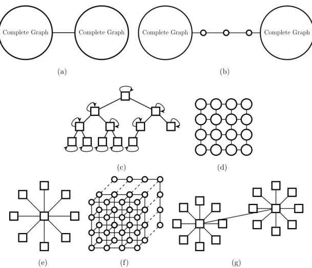
definen(P) as the number of edges in the pathP. A cycleCof a graph _G is a path Psuch that p0 = pl, i.e., the start and end nodes of the path are the same. We denote the period of a directed graph asd(_G), and define it as the greatest common divisor of the length of all cycles in the graph_G. If all edges in the network are bidirectional, we will refer to the graph as undirected. Figure 1.2 shows some examples of common undirected graph topologies.

(24)

Complete Graph Complete Graph

(a)

Complete Graph Complete Graph

(b)

(c) (d)

(e) (f) (g)

Figure 1.2: Examples of common graphs. (a) Dumbbell graph, two complete graphs connected by an edge. (b) Bolas graph, two complete graphs connected by a path. (c) Complete binary tree. (d) 2-d grid or lattice. (e) Star graph. (f) 3-d grid. (g) Two star graph connected on their centers.

Even though we assume the set of nodes in the graph remains constant, we might allow for the edges to change with time. In this scenario, we will refer to the graph as a time-varying

graph and we will define a particular graph at an instant k as _Gk(V, Ek). Moreover, we denote the graph sequence a {Gk}.

Next, we provide three useful definitions regarding the connectivity of a graph, or a se-quence of graphs, for the cases when the edges are directed, undirected, or changing with time.

Definition 1. An undirected and static graph is called connected, if there is a path between any pair of nodes or vertices.

(25)

• Weakly connected if by replacing all directed edges by undirected ones creates a con-nected graph.

• Connected if it contains a directed path, for any two pair of nodes i, j _∈V, from i to

j or from j to i.

• Strongly connected if it contains a directed path, for any two pair of nodes i, j ∈ V, from i to j and from j to i.

Definition 3. A sequence of directed and time-varying graph is called B-strongly connected if there is an integer B ≥1 such that the graph

n

V,S(_ik₌+1)_kBB−1Ei

o

is strongly connected for all k _≥0.

We define the Laplacian matrix L_∈Rn×n _{of the static directed graph} _G _{as a squared} matrix whose elements are defined as

[L]ij =          −1, if (j, i)∈E, deg(i), if i=j, 0, otherwise, where deg(i).

In addition, we will define weighted adjacency matrix A∈ Rn×n _{associated with a graph} G as a squared matrix such that [A]ij 6= 0 if (j, i) ∈ E and [A]ij = 0 if (j, i) ∈/ E. That is, we assume each of the edges in the graph gets assigned a weight. Particularly, we will use positive matrices A where every element is nonnegative. We will say a matrix A is row stochastic or simply stochastic if [A]ij ≥ 0 and Pjn=1[A]ij = 1 for all i ∈ V. Moreover, we will say a matrixAiscolumn stochastic if [A]ij ≥0 andPn_i₌₁[A]ij = 1 for allj ∈V. Finally, a matrix A is doubly stochastic if it is row stochastic and column stochastic.

There are several ways to construct a set of stochastic weight matrices. If the graph is undirected one can construct row stochastic or doubly stochastic weight matrices from undirected local interactions. For example, one can construct doubly stochastic weight matrices by considering a lazy Metropolis (stochastic) matrix of the form ¯Ak = 1₂In+ 1₂Aˆk, where In is the identity matrix and ˆAk is a stochastic matrix whose off-diagonal entries satisfy [ ˆAk]ij =    1 max{di k+1,d j k+1} if (i, j)∈Ek, 0 if (i, j)_∈/Ek,

(26)

where di

k is the degree (the number of neighbors) of node i at time k. Note that the lazy Metropolis weights require undirected communications since each weight [ ˆAk]ij depends on the degree of both agent iand agent j.

Next, we present a series of assumptions for different cases of the network connectivity and directedness. We will use different assumptions for varying directed graphs, time-varying undirected graphs and fixed graphs.

Assumption 1. The graph sequence _{Gk} and the matrix sequence {Ak} are such that:

(a) Ak is doubly-stochastic with [Ak]ij >0 if (i, j)∈Ek.

(b) If (i, j)_∈/ Ek for some i6=j then Aij = 0.

(c) Ak has positive diagonal entries, [Ak]ii>0 for all i= 1, . . . , n.

(d) If [Ak]ij >0, then [Ak]ij ≥η for some positive constant η.

(e) _{Gk} is B-strongly connected.

Assumption 1(a) and Assumption 1(b) characterize the communication between agents. If two agents can exchange information at a certain time instant k, the underlying com-munication graph will have an edge between the corresponding nodes. This also implies a positive weighting of the information shared. The graph sequence _{Gk} and the matrix sequence _{Ak} define a corresponding inhomogeneous Markov chain with transition proba-bilitiesAk. Assumption 1(c) guarantees the aperiodicity of this Markov chain. Additionally, Assumptions 1(d) and 1(e) guarantee that this Markov chain is ergodic by ensuring there is sufficient connectivity and that the entries ofAk do not vanish. Assumption 1 is common in distributed optimization and consensus literature [69, 72]. It guarantees convergence of the associated Markov chain and defines bounds on relevant eigenvalues in terms of the number of agents.

Assumption 2. The graph _G and matrix A are such that:

(a) A is doubly-stochastic with [A]_ij =aij >0 for i6=j if and only if (i, j)∈E.

(b) A has positive diagonal entries, aii>0 for all i∈V.

(c) The graph _G is connected.

Analogous to Assumption 1, we use the following assumption when the interaction between the agents happens over static graphs.

(27)

Assumption 3. The graph sequence _{G_k_} is static (i.e. _G_k = _G for all k) and undirected and the weight matrix A¯ is a lazy Metropolis matrix, defined by

¯ A= 1

2In+ 1 2A,ˆ

where Aˆ is the Metropolis matrix, which is the unique stochastic matrix whose off-diagonal entries satisfy

ˆ Aij =

(

1

max{deg(i)+1,deg(j)+1} if (i, j)∈E,

0 if (i, j)_∈/E.

1.3.2 Lemmas for Left Product of Weighted Adjacency Matrices

One of the main theoretical tools we are going to exploit in the analysis of distributed algorithms over networks is the left product of stochastic matrices. Next, we present a number of auxiliary lemmas that will allow us to analyze the convergence and convergence rate of distributed algorithms. For a more comprehensive account of this results see [95].

First, we recall few results from [72] about the convergence of a product of doubly stochas-tic matrices.

Lemma 1. [72, 69] Under Assumption 1 on a matrix sequence _{Ak}, we have

[Ak:t]ij − 1 n ≤ √ 2λk−t ∀ k ≥t≥0,

where λ∈(0,1) is given by:

λ=1− η 4n2

1

B

.

If each Ak is the lazy Metropolis matrix associated with Gk and B = 1, then λ= 1− 1

O(n2₎.

.

Proof. The proof may be found in [72], except the bounds onλfor the lazy Metropolis chains which may be found in [96].

(28)

Lemma 2. [Corollary 2.a in [72]] Let the graph sequence _{G_k_}, with _G_k = (Ek, V) be

uni-formly strongly connected. Then, there is a sequence _{φ_k_} of stochastic vectors such that

|[Ak:t]ij −φik| ≤Cλk−t for all k≥t ≥0.

The constants C, δ and λ satisfy the following relations: (1) For general B-strongly-connected graph sequences _{Gk},

C = 4, λ = 1− 1 nnB 1 B , δ≥ 1 nnB.

(2) If every graph Gk is regular with B = 1, C =√2, λ = 1₋ 1 4n3 1 B , δ= 1,

and _{Ak} is a sequence of matrices where Ak is a stochastic matrix such that

[Ak]_ij =    1 dj_k if (j, i)∈Ek, 0 otherwise. .

Lemma 3. [Corollary 2.b in [72]] Let the graph sequence _{G_k_} satisfy the B-strong connec-tivity assumption. Define

δ , inf k≥0 min 1≤i≤n[Ak:01n]i . (1.1)

Then, δ _≥ 1/nnB_{, and if all} _G

k with B = 1 are regular, then δ = 1. Furthermore, the

sequence φk from Lemma 2 satisfies φjk ≥δ/n for all k≥0, j = 1, . . . , n.

The next lemma is an extension of Lemma 2 in [45] to the case of time-varying graphs. It provides a technical result that will help us later in the computation of the non-asymptotic convergence rate for the distributed learning algorithms.

Lemma 4. Let Assumption 1 hold for a matrix sequence _{Ak}. Then for all i, k X t=1 n X j=1 [Ak:t]ij − 1 n ≤ 4 log₁₋_λn,

where λ= 1−η/4n2_{, and if every} _A

(29)

Proof. In [45], the authors assume the weight matrix is static and diagonalizable, then they use the following inequality from [97]:

ke0jAk−π0k1 ≤nλ2(A)k,

where ej is a vector with itsj-th entry equal to one and zero otherwise, π is the stationary distribution of the Markov chain with transition matrix A and λ2(A) is the second largest

eigenvalue of the matrix A.

For time-varying graphs, one can use the inequality in Lemma 1 instead. The remainder of the proof remains the same as in [45].

Finally, we will state an enabling theorem presented in [96], which presents a distributed consensus protocol that achieves a consensus with linear growth in the number of agents.

Theorem 5. [96] Suppose each node i in a fixed undirected connected graph updates its variable xi

k at each time instant k ≥2 as follows: yi_k₊₁ =xi_k+1 2 X j∈Ni xj_k₋xi k max_{di_{+ 1, d}j _{+ 1}_}, (1.2a) xi_k₊₁ =y_ki₊₁+ 1₋ 2 9U + 1 y_ki₊₁₋y_ki, (1.2b)

where Ni is the set of neighbors of agentiand di is its corresponding degree. Then, if U ≥n

we have that kyk−x¯1k22 ≤2 1− 1 9U k−1 ky1−x¯1k22 ∀k ≥1, (1.3) where [y_k]i =yki and x¯= n1 n P i=1 xi

1, and the process is initialized with y1i =xi1.

1.3.3 Random Walks, Mixing and Markov chains

Consider a finite graph_G = (V, E) composed ofV nodes with a set of edgesEand a compliant associated row-stochastic matrix A. A random walk on the graph _G is the event of a token moving from one node to another according to some probability distribution. These dynamics are captured by a Markov chain X = (Xk)∞0 such that P{Xk+1 = y|Xk = x} = P(x, y). This Markov chain is calledergodic if it is irreducible and aperiodic. For an ergodic Markov chain, there exists a unique stationary distribution π, which describes the probability that

(30)

a random walk visits a particular node in the graph as the time goes to infinity, that is

P{Xk = j} → πj as k → ∞. The stationary distribution is invariant to the transition matrix, that is π0_P ₌ _π0_{. It follows immediately that its convergence reduces to analyzing} powers of P (Theorem 4.9 in Levin et al.[98]).

Now, define the distance to stationarity as d(k) = max

x∈Ω kP

k_(x,

·)₋π_kT V. Moreover, define the mixing time of the Markov chain as

tmix() = min

k {k:d(k)≤},

and we say the Markov chain is rapid mixing if tmix() = poly(logn,log1). Finally, it holds

that λ2 2(1₋λ2) log 1 2 ≤tmix()≤ logn+ log(1/) 1₋λ2 , (1.4)

where λ2 is the second largest left-eigenvalue of the transition matrix P [99].

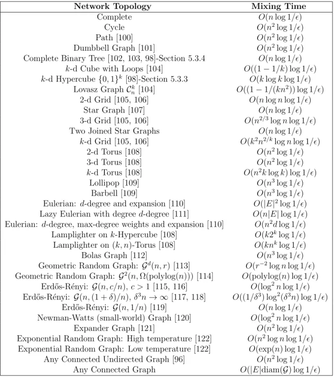
Table 1.1 shows estimates for the dependency of the mixing time of a random walk on a graph for several common well-studied topologies and the number of nodes in the network.

1.3.4 The Coupling Method

Consider two independent Markov chains X = (Xk)∞0 and Y = (Yk)∞0 , with the same

transition matrixP. Then, define the coupling time K as the smallest k such thatXk=Yk, that is, K = mink≥0{Xk = Yk}. Note that K is a random variable and it depends on P as well as the initial distributions of the processes Xk and Yk. Finally, define the quantityLP as the maximum expected coupling time of a Markov chain with transition matrix P over all possible initial distributions of the processes Xk and Yk, then

LP = max

u,v E[K] where X0 =u and Y0 =v.

In words, this LP is the maximum expected time it takes for two random walks, with the same transition matrix and arbitrary initial states, to intersect. If we assumeX starts from a distribution π, and Y from some other arbitrary stochastic vector v and we couple the

(31)

Table 1.1: Maximum expected convergence time for a random walk on networks with n nodes.

Network Topology Mixing Time

Complete O(nlog 1/)

Cycle O(n2_{log 1/)}

Path [100] O(n2_{log 1/)}

Dumbbell Graph [101] O(n2_{log 1/)}

Complete Binary Tree [102, 103, 98]-Section 5.3.4 O(nlog 1/) k-d Cube with Loops [104] O((1₋1/k) log 1/) k-d Hypercube {0,1}k _{[98]-Section 5.3.3} _O(k_log_k_{log 1/)}

Lovasz Graph Ck

n [104] O((1−1/(kn2)) log 1/)

2-d Grid [105, 106] O(nlognlog 1/)

Star Graph [107] O(nlog 1/)

3-d Grid [105, 106] O(n2/3_log_n_{log 1/)}

Two Joined Star Graphs O(nlog 1/)

k-d Grid [105, 106] O(k2_n2/k_log_n_{log 1/)}

2-d Torus [108] O(n2_{log 1/)}

3-d Torus [108] O(n2_{log 1/)}

k-d Torus [108] O(n2_k_log_{k) log 1/)}

Lollipop [109] O(n3_{log 1/)}

Barbell [109] O(n3_{log 1/)}

Eulerian: d-degree and expansion [110] O(_|E_|2_{log 1/)}

Lazy Eulerian with degree d-degree [111] O(n_|E_|log 1/) Eulerian: d-degree, max-degree weights and expansion [110] O(n2_d_{log 1/)}

Lamplighter on k-Hypercube [108] O(k2k_{log 1/)} Lamplighter on (k, n)-Torus [108] O(knk_{log 1/)}

Bolas Graph [112] O(n3_{log 1/)}

Geometric Random Graph: _Gd_{(n, r) [113]} _O(r₋2_log_n_{log 1/)}

Geometric Random Graph: _G2_(n,_{Ω(polylog(n))) [114]} _{O(polylog(n) log 1/)}

Erd˝os-R´enyi: _G(n, c/n), c >1 [115, 116] O(log2nlog 1/) Erd˝os-R´enyi: _G(n,(1 +δ)/n), δ3_n

→ ∞ [117, 118] O((1/δ3_{) log}2_(δ3_{n) log 1/)}

Erd˝os-R´enyi: G(n,1/n) [119] O(nlog 1/) Newman-Watts (small-world) Graph [120] O(log2nlog 1/)

Expander Graph [121] O(n2_{log 1/)}

Exponential Random Graph: High temperature [122] O(n2_log_n_{log 1/)}

Exponential Random Graph: Low temperature [122] O(exp(n) log 1/) Any Connected Undirected Graph [96] O(n2_{log 1/)}

Any Connected Graph O(_|E_|diam(_G) log 1/) processes Y and X by defining a new processW such that

Wk =    Yk, if k < K, Xk, if k ≥K,

(32)

then

kv0Pk−πk1 ≤max

v Pv{K > k} and by the Markov inequality

kv0Pk−πk1 ≤

maxvE[K] k .

Thus, afterT =O(LP log 1/) steps, kvTPT −πk1 ≤, for any v.

1.3.5 Some Basic Notions on Convex Analysis

In this subsection, we will present a sequence of basic definitions from convex analysis. For a comprehensive account of definitions and results of convex analysis see [123].

Definition 4 (Definition 1.2.1 in [123]). A subset C of Rd is called convex if

αx+ (1₋α)y _∈C, _∀x, y _∈C,_∀α_∈[0,1].

Definition 5 (Definition 1.2.2 in [123]). Let C be a convex subset of Rd. A function

f :C _→R is called convex if

f(αx+ (1−α)y)≤αf(x) + (1−α)f(y), ∀x, y ∈C,∀α∈[0,1].

Definition 6. Let f :Rd_→_R _{be a convex function and} _X _{be a bounded set in} _Rd_{. We say} f is Lipschitz continuous over X with constant L, or simply L-Lipschitz over X, if

kf(x)−f(y)k ≤Lkx−yk, ∀x, y ∈X.

Definition 7. We will refer to a function f(·) as µ-strongly convex with µ >0, if for any

x, y it holds that

f(y)≥f(x) +D∇˜f(x), y−xE+µ

2kx−yk

2 2,

where _∇˜f(x) is any subgradient of f(_·) at x.

(33)

(or L-smooth), if it is differentiable and for any x and y it holds that

k∇f(x)− ∇f(y)k2 ≤Lkx−yk2.

1.3.6 Additional Definitions

McDiarmid’s Inequality

In the proof of some of the non-asymptotic converge rates bounds we will use McDiarmid’s inequality [124], which provides bounds for the concentration of functions of random vari-ables. This inequality allows us to show bounds on the probability that the beliefs exceed a given value . For completeness, next, we state the McDiarmid’s inequality.

Theorem 6. (McDiarmid’s inequality [124]) Let X1, . . . , Xk be a sequence of independent

random variables with Xt ∈ X for 1 ≤ t ≤ k. Further, let g : Xk → R be a function of

bounded differences, i.e., for all 1_≤t_≤k,

sup xt∈X

g(. . . , xt, . . .)− inf xt∈X

g(. . . , xt, . . .)≤ct,

then for any >0 and all k_≥1,

Pg({Xt}k_t₌₁)−E[g({Xt}k_t₌₁)]≥ ≤exp − 2 2 Pk t=1c2t ! .

Distances between Probability Distributions

Next, we provide three definitions of the most common “distance” functions between prob-ability distributions.

Definition 9. The squared Hellinger distance between two probability distributions P and

Q is given by h2(P, Q) = 1 2 Z r dP dλ − r dQ dλ !2 dλ,

where P and Q are dominated by λ. Moreover, the Hellinger distance satisfies the property that 0_≤h(P, Q)_≤1.

(34)

Definition 10. If P and Q are probability measures over a set X, and P is absolutely continuous with respect toQ, then the Kullback-Leibler divergence from Q toP is defined as

DKL(PkQ) =

Z

X

logdP dQdP,

where dP/dQ is the Radon-Nikodym derivative of P with respect to Q.

Definition 11. The total variation distance between two probability measures P and Q on a sigma-algebra _F of subsets of the sample space Ω is defined as

kP ₋Q_kT V = sup A∈F|

P(A)₋Q(A)_|.

The Kronecker Product

In the next definition, we recall some basic properties of the Kronecker product and the corresponding Kronecker product of two graphs.

Definition 12. [125] Let A be a m×n matrix, and C be a p×q matrix, the Kronecker product A_⊗C is the mp_×nq matrix defined as:

A_⊗C =     a11C . . . a1nC .. . . .. ... am1C . . . amnC     or explicitly A⊗C =                a11     c11 . . . c1q .. . . .. ... cp1 . . . cpq     . . . a1n     c11 . . . c1q .. . . .. ... cp1 . . . cpq     .. . . .. ... am1     c11 . . . c1q .. . . .. ... cp1 . . . cpq     . . . amn     c11 . . . c1q .. . . .. ... cp1 . . . cpq                   

(35)

=                  a11c11 . . . a11c1q . . . a1nc11 . . . a1nc1q .. . . .. ... ... . .. ... a11cp1 . . . a11cpq . . . a1ncp1 . . . a1ncpq .. . ... ... ... .. . ... ... ... am1c11 . . . am1c1q . . . amnc11 . . . amnc1q .. . . .. ... ... . .. ... am1cp1 . . . am1cpq . . . amncp1 . . . amncpq                  .

Moreover, the following properties hold:

1. Bilinearity and associativity: for matrices A, B and C, and a scalar k, it holds:

A_⊗(B+C) =A_×B+A_⊗C (A+B)×C=A⊗C+B⊗C

(kA)_⊗C=A_⊗(kB) =k(A_⊗B) (A_⊗B)_⊗C=A_⊗(B_⊗C).

2. Non-Commutative: In general A_×B ₆= B _⊗A. However, there exists commutation matrices P and Q such that:

A_⊗B =P(B_⊗A)Q,

and if A and B are square matrices then P =Q0_.

3. Mixed-product property: for matrices A, B, C and D:

(A_⊗B)(C_⊗D) = (AC)_⊗(BD).

Additionally, we will define the Kronecker product of graphs as follows. The Kronecker (also known as categorical, direct, cardinal, relational, tensor, weak direct or conjunction) product _G = G1⊗ G2 of two graphs G1 = (V1, E1) and G2 = (V1, E1) is a graph G = (V, E)

where V =V1 ×V2 and |V|= |V1||V2|; and (u, u0)→ (v, v0) ∈E if and only if u →v ∈ E1

and u0 _→_v0 _∈_E

2. Moreover, the adjacency matrix of the graph G is the Kronecker product

(36)

CHAPTER 2 GRAPH-THEORETIC ANALYSIS OF BELIEF

SYSTEMS UNDER LOGIC CONSTRAINTS

In this chapter, we study how the structural properties of the social network of agents and the set of logic constraints influence the dynamics of a belief system from agraph-theoretic point of view. We describe this influence for the convergence of beliefs, the expected convergence time and the stationary value of the belief system. Informally, we answer the following three questions with graph-theoretic conditions that are easily accessible for a number of commonly used topologies in large-scale complex networks:

1. When does a belief system converge?

2. How long does it take for a belief system to converge? 3. Where does a belief system converge?

2.1 Problem Formulation

Friedkin et al.[37, 38] describe a belief system with logic constraints as a group of n agents that periodically exchange and update their opinions about a set ofm different truth state-ments with logical dependencies among them. After each social interaction, the agents use shared opinions as well as underlying logical dependencies among the opinions to update their beliefs. The agents exchange their opinions by interacting over a social network cap-tured by a graph G = (V, E), where V is the set of agents, and E is a set of edges. A directed edge towards an agent indicates that it receives the opinion of another agent, i.e., the directed flow of information. Analogously, the logical dependencies among the truth statements are modeled by a graph _T = (W, D), where an edge between two statements exists if the belief in one statement affects belief in the other.

The generalized dynamics of a belief system are defined as follows. First, every agent aggregates its opinions on every truth statement according to the imposed logic constraints (i.e., modifying the opinions to take into account the dependencies on the other truth state-ments). Second, the agents share their opinions over a social network, where the opinions

(37)

are aggregated again to take into account those coming from the neighboring agents (i.e., social interactions). Finally, a new opinion is formed as a combination of the most recent aggregation and the initial opinion, which models adversity to deviate from the initial beliefs or stubbornness. The opinion of an agent on a specific statement being true or false is mod-eled by a scalar value between zero and one. A value of zero indicates that the given agent strongly believes a specific statement is false, whereas a value of one indicates that the agent believes the statement is true. Similarly, a value of 0.5 indicates the maximal uncertainty about a statement. The aggregation steps consist of weighted (convex) combinations of the available values, where the weights represent the relative influence. This model is described in the following equations (2.1) for an arbitrary agent i ∈ V and an arbitrary statement u_∈W: ˆ xi_k(u) = m X v=1

Cuvxik(v) (Aggregation by logic constraints) (2.1a) ¯

xi_k(u) = n

X

j=1

Aijxˆjk(u) (Aggregation by social network) (2.1b) xi_k₊₁(u) = λix¯_ki(u) + (1−λi)xi₀(u) (Influence of initial beliefs) (2.1c) where 0≤xi

k(u)≤1 represents the opinion of an agentiat timek on a certain statementu, while ˆxi

k(u) and ¯xik(u) are the intermediate aggregation steps. Specifically, the intermediate aggregated opinion ˆxi

k(u) of agent i on statement u is formed by using the opinions of the same agent about the other statements v. The parameters 0 _≤ Cuv ≤ 1 are compliant with the graph _T that models the logic constraints in the sense that Cuv is nonzero if the statement u depends on statement v, and otherwise Cuv = 0. These parameters represent the strength of the logic constraints, i.e., the influence that an opinion on a statement has on the opinion on other statements.

Subsequently, the intermediate aggregated opinion ¯xi

k(u) of agent i on statement u is formed by combining all the intermediate opinions ¯xi

k(u) of neighboring agents j. In this update, the parameters 0 ≤ Aij ≤ 1 represent the weights that an agent i assigns to the information coming from its neighborj, for exampleA13is how agent 1 weights the opinions

shared by agent 3. These parameters are compliant with the network _G in the sense that if there is an incoming edge to agent i from agent j in the graph, then the corresponding weight Aij is nonzero.

The last update in Eq. (2.1) indicates that, at timek+1, the new opinionxi

k+1(u) of agenti

on statementuis obtained as a weighted combination of its intermediate aggregated opinion ¯

xi

(38)

agent i uses models its stubbornness. If λi _< _{1 we say an agent is} _stubborn_{, where} _λi _{= 0} indicates that the agenti ismaximally closed to the influence of others. If λi _{= 1, agent} _i_is said to be maximally open to the influence of others, and oblivious if additionally it is not influenced by stubborn agents.

We can group the parameters_{Aij}into ann-by-nmatrixA, known as thesocial influence

structure, and the parameters {Cuv} into an m-by-m matrix C, known as the multi-issues

dependent structure [38]. These matrices are nonnegative. Furthermore, the weights Aij assigned by an agent i to its neighbors j sum up to one, i.e., the sum of the entries in each row of the matrix A is 1; likewise, the sum of the entries in each row of the matrix C is 1. Thus, the matrices A and C are row-stochastic

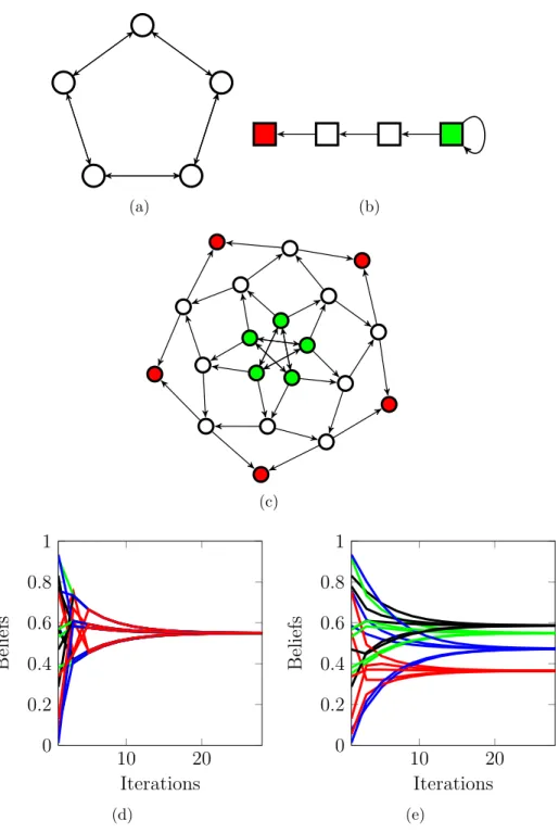
Figure 2.1(c) shows the belief system generated by the network of agents in Fig. 2.1(a) and the set of logic constraints in Fig. 2.1(b). This new graph depicted in Fig. 2.1(c) is much larger than the network of agents or the network of statements taken separately; effectively, it has 2nmnodes. The belief of each agent on each truth statement is a separate node; also, the initial beliefs are separate nodes.

The model of this larger graph of the belief system can be compactly restated as

xk+1 =P xk, (2.2)

wherexk ∈[0,1]2nm is a state that stacks the current beliefs of all agents on all topics along side with the initial beliefs, i.e.,

xk= x1_k(1), . . . , x1_k(m) | {z } Beliefs of Agent 1 , x2_k(1), . . . , x2_k(m) | {z } Beliefs of Agent 2 , . . . , xn_k(1), . . . , xn_k(m) | {z } Beliefs of Agentn , x1₀(1), . . . , x1₀(m) | {z }

Initial Beliefs of Agent 1

, x2₀(1), . . . , x2₀(m)

| {z }

Initial Beliefs of Agent 2

, . . . , xn₀(1), . . . , xn₀(m)

| {z }

Initial Beliefs of Agentn

0 and P = " (ΛA)_⊗C (In₋Λ)_⊗Im 0nm Inm # ,

where0nm is a zero matrix of sizen×m,Inmis an identity matrix of sizen×m,⊗indicates the Kronecker product, Λ is a diagonal matrix with the i-th diagonal entry being λi_{, and} x0 _{denotes the transpose of a vector or matrix} _{x. This allows for the definition of the belief} system graph _P, which is compliant with the matrix P, where an edge from ` to r exists if Pr` >0. Equation (2.3) shows an example of a matrix P for the belief system in Fig. 2.1(c)

(39)

1 2 3 4 A=     0 0 1 0 1 2 1 4 0 1 4 0 0 0 1 0 0 0 1     (a) 1 2 3 C =   1 2 1 2 0 0 0 1 0 0 1   (b) x1k(1) x1k(2) x1k(3) x10(3) x1 0(2) x1 0(1) 1 2 3 4 (c)

Figure 2.1: A belief system with 4 agents and 3 truth statements. (a) Agents are

represented as nodes/circles, numbered from 1 to 4, and the network of influences among them is shown as edges between nodes. The truth statements or topics are color-coded, e.g., the truth statement 1 is represented as a red square. Agent 2 is influenced by its own opinion and agents 4 and 1, agent 1 follows the opinion of agent 3 which in turn follows the opinion of agent 4, agent 4 follows its own opinion only. A possible matrix A for this social network is shown below the graph. This indicates that agent 2 assigns a higher weight of 1

2

to the opinion of agent 1 than the weight it assigns to the opinion of communicated by agent 4. (b) The truth statement 1 is influenced by the belief that statement 2 is true, statement 2 directly follows the belief in statement 3. A possible matrixC for this set of logic constraints is shown below the graph. The belief that the truth statement 1 is true is influenced (with a weight of 1₂) by the opinion that the truth statement 2 is true. (c) The beliefs system, see equation 2.2, composed by the agent’s interaction graph and the logic constraints.