Deep learning for texture and dynamic texture analysis

dynamic texture analysis

Vincent Andrearczyk

Supervisor: Prof. Paul F. Whelan

School of Electronic Engineering

Dublin City University

This dissertation is submitted for the degree of

Doctor of Philosophy

I hereby certify that this material, which I now submit for assessment on the pro-gramme of study leading to the award of Doctor of Philosophy is entirely my own work, and that I have exercised reasonable care to ensure that the work is original, and does not to the best of my knowledge breach any law of copyright, and has not been taken from the work of others save and to the extent that such work has been cited and acknowledged within the text of my work.

Vincent Andrearczyk September 2017

I would like to first thank Prof. Paul Whelan for giving me the opportunity to pursue this research program and for his support and guidance throughout the past four years. I also want to express my gratitude to Dr. Ovidiu Ghita for his precious advice and interest in my work during the first two years.

I wish to thank all the members of the Centre for Image Processing and Analysis (CIPA) for making this period enjoyable and memorable. In particular, I thank Dr. Tony Marrero and Dr. Ram Prasad for sharing their valuable experience and suggestions. I am also grateful to my friends and former colleagues in DCU Chris and Vidak for their help.

I would like to thank my brother and my family for the precious time spent at home and in Castres, as well as my friends Florian, Kevin, Pierre, Sebastien, Thibaud, and Xavier.

I want to offer a special thank to Sonja whose support, love, patience, and help have been essential to the completion of this work.

Enfin, je remercie ma mère pour son soutien et son amour inconditionnel, dépourvu de jugement et d’attentes. Son état d’esprit et sa bonté sont de riches sources d’inspiration.

Vincent Andrearczyk and Paul F. Whelan (2017), Texture segmentation with Fully Convolutional Networks", arXiv preprint arXiv:1703.05230.

Vincent Andrearczyk and Paul F. Whelan (2017), Convolutional Neural Network on Three Orthogonal Planes for Dynamic Texture Classification, Under review at Pattern Recognition, subject to minor revisions, arXiv preprint arXiv:1703.05530.

Vincent Andrearczyk and Paul F. Whelan (2016), Using Filter Banks in Convo-lutional Neural Networks for Texture Classification,Pattern Recognition Letters, vol. 84, pp. 63–69.

Book Chapter Publication

Vincent Andrearczyk and Paul F. Whelan (2017), Deep Learning in Texture Analysis and its Application to Tissue Image Classification, Biomedical Texture Analysis (BTA), Fundamentals, Tools and Challenges (Academic Press, London, 2017), Edi-tors: Adrien Depeursinge, Omar S. Al-Kadi and J. Ross Mitchell, In Press, Published Date: 1st October 2017.

Conference Publications

Vincent Andrearczyk and Paul F. Whelan (2016), Deep Learning for Biomedical Texture Image Analysis,Irish Machine Vision and Image Processing Conference (IMVIP).Best Overall Paper Award

Vincent Andrearczyk and Paul F. Whelan (2015), Dynamic Texture Classification using Combined Co-Occurrence Matrices of Optical Flow,Irish Machine Vision and Image Processing Conference (IMVIP).Best Overall Paper Award

List of figures xiii

List of tables xix

List of abbreviations xxi

1 Introduction 1

1.1 Texture and dynamic texture analysis . . . 1

1.1.1 What is texture? . . . 1

1.1.2 What is dynamic texture? . . . 3

1.1.3 Analysis and applications . . . 4

1.1.4 Challenges . . . 5

1.1.5 Classic approaches . . . 7

1.2 Motivation for the thesis . . . 8

1.3 Thesis summary and main contributions . . . 9

1.4 Outline of the dissertation . . . 10

2 Literature review 13 2.1 Introduction . . . 13

2.2 Texture analysis . . . 13

2.2.1 Texture perception . . . 13

2.2.2 Classic texture feature extraction . . . 14

2.2.3 Texture analysis problems . . . 34

2.2.4 Deep descriptor and deep learning in texture analysis . . . . 37

2.3 Dynamic texture analysis . . . 40

2.3.1 Classic dynamic texture analysis . . . 40

2.3.2 Deep learning in dynamic texture analysis . . . 42

3 Convolutional networks for texture classification 45 3.1 Introduction . . . 45

3.2 Material and Methods . . . 46

3.2.2 Details of the network . . . 48

3.3 Datasets and experimental setups . . . 48

3.4 Results and discussion . . . 50

3.4.1 Networks from scratch and pre-trained . . . 50

3.4.2 Networks depth analysis . . . 51

3.4.3 Domain transferability . . . 52

3.4.4 Visualisation . . . 53

3.4.5 Results on larger images . . . 55

3.4.6 Combining texture and shape analyses . . . 55

3.4.7 Deeper Texture CNN . . . 57

3.4.8 Discussion . . . 58

3.5 Application to biomedical tissue images . . . 58

3.5.1 Motivation . . . 58

3.5.2 State of the art . . . 58

3.5.3 Method . . . 59

3.5.4 Experiments . . . 60

3.5.5 Results . . . 62

3.5.6 Discussion . . . 64

4 Dynamic texture recognition with convolutional networks 65 4.1 Introduction . . . 65

4.2 Materials and Methods . . . 66

4.2.1 Texture CNN . . . 66

4.2.2 Dynamic Texture CNN . . . 68

4.2.3 Domain transfer . . . 70

4.3 Datasets and experimental setups . . . 71

4.3.1 Datasets . . . 71

4.3.2 Implementation details . . . 73

4.4 Results and discussion . . . 73

4.4.1 Results . . . 73

4.4.2 Contribution of the planes . . . 77

4.4.3 Domain transferability and visualisation . . . 80

4.5 Discussion . . . 82

5 Texture segmentation with fully convolutional networks 83 5.1 Introduction . . . 83

5.2 Material and Methods . . . 84

5.2.1 Network architecture . . . 84

5.2.2 Refinement of segmented regions . . . 85

5.3.1 Experiment A: Supervised training with multiple training

images per class . . . 86

5.3.2 Experiment B: Supervised training with single training im-age per class . . . 90

5.3.3 Experiment C: Unsupervised training . . . 91

5.4 Discussion . . . 95

6 Conclusions and future work 97 6.1 Contributions and conclusions . . . 97

6.1.1 List of contributions . . . 98

6.1.2 Limitations of deep learning . . . 101

6.2 Future Work . . . 103

References 105 Appendix A Introduction to deep learning and convolutional neural net-works 121 A.1 Introduction . . . 121

A.1.1 Overview . . . 121

A.1.2 Definitions . . . 121

A.1.3 Motivation . . . 122

A.2 Neural networks . . . 123

A.2.1 The neuron . . . 123

A.2.2 Artificial neural network architecture . . . 125

A.2.3 Training a neural network: Backpropagation . . . 127

A.2.4 Regularisation methods . . . 135

A.2.5 Recurrent neural networks . . . 137

A.2.6 Unsupervised learning . . . 138

A.2.7 Reinforcement learning . . . 140

A.3 Deep learning . . . 141

A.3.1 Regularisation . . . 142

A.3.2 Vanishing gradients . . . 142

A.3.3 Internal covariate shift . . . 143

A.3.4 Batch normalisation . . . 143

A.3.5 Deep recurrent networks . . . 143

A.3.6 Deep unsupervised methods . . . 145

A.4 Convolutional neural networks . . . 146

A.4.1 Overview . . . 146

A.4.2 Brief history . . . 147

A.4.4 Regularisation . . . 155

A.4.5 CNN architectures . . . 155

A.4.6 Applications . . . 162

1.1 Examples of texture images from the kth-tips-2b database [22]. (a) cork, (b) wood, (c) linen, (d) wool, (e) lettuce, (f) aluminum foil and (g) white bread. . . 2 1.2 Examples of DT sequences from the DynTex database [24] of the

following classes: (a) sea, (b) traffic and (c) trees. . . 3 1.3 Examples of segmentation problems. (a) Image from the Prague

texture segmentation benchmark [26]: mosaic with six texture re-gions, (b) texture mosaic generated from Kylberg texture images [31] including five texture regions, and (c) highly textured zebra skin and grass background. . . 4 1.4 A texture distortion resulting in patterns of varying sizes, shapes

and frequency. (a) Water ripples appear at different scales and frequencies due to the camera angle to the surface normal, and (b) Fisheye effect on bricks texture due to image acquisition. . . 7 2.1 An example of GLCM computation with a small texture region and

four grey levels [10]. The distance between neighbours isd=1 and the orientation isθ =0. . . 17

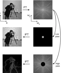
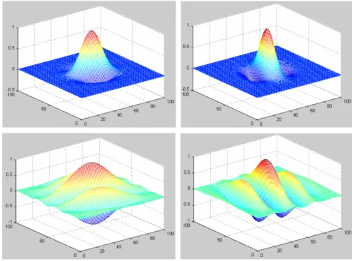
2.2 An example of Fourier transforms and inverse Fourier transforms (after low-pass and high-pass filters in the frequency domain). Left: spatial domain; right: frequency domain (magnitude of Fourier spectrum). . . 20 2.3 2D Gabor filters for 30°(left) and 120°(right) orientations. Top row:

scaleσx=σy=1.0, central frequency f0=1.5/2π; bottom row:

scaleσx=σy=2.0, central frequency f0=2.5/2π. . . 22

2.4 A Gabor filter bank in the frequency domain. The set is composed of filters at five scales and four orientations with a total of 20 filters, each resulting in a centre-symmetric pair of lobes. The axes are in normalised frequencies. Figure reproduced from [48]. . . 23

2.5 A three-level DWT filter bank computing a cascade of high-pass and low-pass filters followed by downsampling, successively decompos-ing the image into multiple frequency components. . . 23 2.6 A 2D DWT in more detail with high-pass and low-pass filters applied

separately horizontally (Hirows,Lorows) and vertically (Hicol,Locol). 24 2.7 A Three-level DWT pyramidal decomposition of an image. Figure

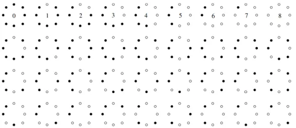
reproduced from [81]. . . 24 2.8 The original LBP histogram extraction [12]. . . 25 2.9 The 36 possible rotation invariantLBP₈ri_,R. The nine uniform LBPs

(LBP₈riu2_,R ) are depicted in the first row. Figure reproduced from [13]. 27 2.10 Training and testing phases in a texture classification framework.

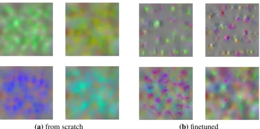
Note that the feature extraction is learned from the training data in optimised filters and dictionary learning methods as represented by the dashed arrow. . . 34 3.1 A T-CNN architecture with three convolution layers (T-CNN3). . . . 47 3.2 Examples of activation maximisation of neurons in the third

convo-lution layer. The T-CNN3 networks are trained on kth-tips-2b (a) from scratch and (b) finetuned (pre-trained on ImageNet). Figures obtained with the DeepVis toolbox [170]. . . 54 3.3 Examples of activation maximisation of neurons in the last

fully-connected layer (FC3). The T-CNN3 networks are trained on kth-tips-2b (a) from scratch and (b) finetuned (pre-trained on ImageNet). Figures obtained with the DeepVis toolbox [170]. . . 54 3.4 The architecture of the Texture and Shape CNN (TS-CNN-3),

inte-grating T-CNN3 to a classic CNN (AlexNet). . . 56 3.5 Training and testing phases of the developed collective T-CNN

method with subimages and scoring vote. . . 60 3.6 Examples of H&E stained tissue images from the IICBU dataset

[175] (a) mice tissue liver images (AGEMAP) and (b) Lymphoma tissue images. . . 62 4.1 An overview of the proposed DT-CNN for the classification of a

DT sequence based on T-CNNs on three orthogonal planes in an ensemble model approach. The T-CNNs separately classify slices extracted from three planes of a DT sequence. The outputs of the last fully-connected layers are summed and the highest score gives the collective classification decision. . . 66 4.2 A diagram of the DT sequence slicing in three orthogonal planes. . . 68

4.3 Examples of DT slices in three orthogonal planes of foliage, traffic and sea sequences from the DynTex database. (a)xy(spatial), (b)xt (temporal) and (c)yt (temporal). . . 71 4.4 A misclassified sequence of the DynTex beta dataset and examples

from the true class and from the detected one. (a) misclassified sequence, (b) true class “rotation” and (c) detected class “trees”. . . 75 4.5 A misclassified sequence of the DynTex gamma dataset and

exam-ples from the true class and from the detected one. (a) misclassified sequence, (b) true class “naked trees” and (c) detected class “foliage”. 75 4.6 Classification rates of individual classes of the Dyntex++ dataset

with the proposed DT-CNN approach (DT-AlexNet). . . 76 4.7 Classification rates of individual classes using singlexy,xt, andyt

planes with DT-AlexNet on the (a) ucla-8 and (b) ucla-9 sub-datasets. 79 4.8 Classification rates of individual classes using singlexy,xt, andyt

planes with DT-AlexNet on the (a) DynTex beta and (b) DynTex gamma sub-datasets. . . 79 4.9 Classification rates of individual classes of the Dyntex++ dataset

using singlexy,xt, andyt planes with DT-AlexNet. . . 80 4.10 Classification rates of DT-AlexNet with networks trained from scratch

vs. pre-trained on ImageNet with the following planes: (a)xy+xt+yt (b) xy, (c) xt and (d) yt. . . 81 5.1 The FCNT architecture inspired from [6]. The grids reveal the

rela-tive spatial coarseness of pooling and prediction layers. Convolution layers are depicted as vertical lines. Skip connections, represented by arrows, allow the network to combine local information from early layers with more global information extracted by deeper layers (conv6). Diagram adapted from [6]. . . 85 5.2 Examples of segmentation with FCNT on the supervised Prague

texture segmentation task (experiment B) and comparison with the state of the art (see Section 5.3.2 for more details on the state of the art methods). The models are trained with one image per texture segment (six training images in this example). (a) Input image to segment; (b) ground truth segmentation; (c) Markov Random Field (MRF) segmentation [120]; (d) Co-Occurrence Features (COF) segmentation; (e) Con-Col segmentation; (f) FCNT segmentation without refinement; (g) FCNT segmentation with refinement. Best viewed in colour. . . 87

5.3 Examples of segmentation results with FCN8 [6] and with the de-veloped FCNT on experiment A (Kylberg-seg). First row: input test image to segment; second row: ground truth segmentation; third row: FCN8 segmentation; fourth row: FCNT segmentation. Best

viewed in colour. . . 89

5.4 Examples of segmentation results using different methods on the Prague unsupervised dataset. (a) Input image with superimposed ground truth boundaries; (b) FCNT segmentation with K-means train-ing; (c) FSEG segmentation; (d) FCNT segmentation with FSEG pre-segmentation; (e) PCA-MS segmentation; (f) FCNT segmen-tation with PCA-MS pre-segmensegmen-tation; (f) PMCFA segmensegmen-tation; (g) FCNT segmentation with PMCFA pre-segmentation; (h) MK segmentation; (i) FCNT segmentation with MK pre-segmentation; Best viewed in colour. . . 94

A.1 A perceptron linear neuron: first developed artificial neuron. . . 123

A.2 An illustration of a weightaand biasbin a line equation example ax+b. . . 124

A.3 A recent neuron with activation function. . . 124

A.4 A commonly used non-linear activation functions. . . 125

A.5 A three layer Multi Layer Perceptron. . . 126

A.6 The architecture of anL−1 layers neural network (L layers including the input). . . 126

A.7 A 1D gradient descent minimisation of f(w)with (a) global mini-mum, (b) local minimum. . . 132

A.8 An example of overfit (blue curve). . . 136

A.9 An illustration of overfitting the training data and early stopping method by evaluation of the model on an unknown validation set during training. . . 136

A.10 A graph representing a basic fully recurrent network. Note that the inputs, weights, hidden states, and outputs are vectors. (a) graph with a loop feeding the previous hidden state back into the network, (b) unfolded graph over time. . . 138

A.11 The architecture of a simple AE. . . 140

A.12 The architecture of a Restricted Boltzmann Machine with three input and four hidden neurons including forward (left) and backward passes (right). . . 141

A.14 An illustration of the GAN structure. The generative model Gis trained to generate samples that seem to originate from the real training data (i.e. maximise the discriminator’s error), while the dis-criminative modelDis trained to discriminate the generated samples from the training data (i.e. minimise the error). . . 146 A.15 A basic overview of a Convolutional Neural Network architecture. . 147 A.16 An illustration of the receptive field of a neuron after three

convolu-tion layers. The receptive field of the neuronnis the red area in the input image connected to this neuron through the convolutions. Best viewed in colour. . . 148 A.17 A timeline of CNN history. . . 149 A.18 A convolution layer with two input channels and three output feature

maps. The activation functions are not represented for simplicity. . . 151 A.19 An illustration of the filter size, stride and zero padding in the

for-ward pass of a convolution layer.W andHare respectively the width and height of the input channel. . . 152 A.20 An example of a pooling layer (Forward pass) with 2×2 filters (a)

max pooling, (b) average pooling. . . 154 A.21 The LeNet5 architecture. Image replicated from [5]. . . 156 A.22 The AlexNet architecture. Image replicated from [15]. . . 156 A.23 The R-CNN object detection framework. Image replicated from [213].157 A.24 A basic FCN architecture with pixelwise prediction. The

upsam-pling, deconvolution, and skip layers are not specified and only the prediction image is represented. Image replicated from [213]. . . 158 A.25 A comparison of (a) a convolution layer and (b) a Network in

Net-work block (Mlpconv). Image replicated from [215]. . . 159 A.26 An inception module used in GoogleNet. Image replicated from [164].160 A.27 The GoogleNet architecture. Convolution layers are depicted in

blue, pooling layers in red, softmax in yellow, concatenation and normalisation in green and finally, input and labels in white. Image replicated from [164]. . . 160 A.28 A residual learning block. Image replicated from [210]. . . 161 A.29 A visualisation of filters and responses of the neurons in the first

convolution layer of AlexNet trained on ImageNet. (a) Input image, (b) filters, (c) responses. Figures obtained with the DeepVis toolbox [170]. . . 162

A.30 A visualisation of several features learned by neurons in AlexNet trained on ImageNet and their response to an input image. The first column depicts the response of a particular neuron. The second col-umn shows the image patches which maximally activate this neuron. The third and fourth columns show the deconvolution images and the images obtained by activation maximisation respectively. (a) input image, (b) two neurons in Conv1, (c) two neurons in Conv2, (d) two neurons in Conv5. Figures obtained with the DeepVis toolbox [170]. Note that the deeper receptive fields are larger than shallow ones but are resized for display. . . 165

3.1 Classification accuracy (%) of various networks trained from scratch and finetuned (pre-trained on ImageNet). The number of trainable parameters (in millions) is indicated in brackets for 1,000 classes. The state of the art results are as reported by the authors in the

original papers. . . 50

3.2 Accuracy (%) of various network depths with average and maximum pooling of the energy layer. . . 51

3.3 Classification results (accuracy %) on the kth-tips-2b dataset using networks pre-trained on different databases. . . 52

3.4 Accuracy (%) of the T-CNN3 and comparison with the literature. . . 55

3.5 Classification results (accuracy %) on kth-tips-2b using AlexNet and T-CNN3 separately and combined as well as the state of the art method with a medium depth CNN (VGG-M). The number of trainable parameters in millions is indicated in brackets for 1,000 classes. . . 56

3.6 Classification results (accuracy %) on the kth-tips-2b dataset using T-CNN based on GoogleNet. . . 57

3.7 Classification accuracy (%) of the collective T-CNN and comparison with the state of the art on the 10-fold cross-validation setups. The WND-CHARM results are obtained from a hold-25%-out validation. 63 3.8 Classification accuracy (%) and Mean Average Precision (MAP) (%) of the collective T-CNN and comparison with the state of the art on other validation setups. . . 63

3.9 Confusion matrix of the collective T-CNN on Lymphoma-5p. . . 64

3.10 Confusion matrix of the collective T-CNN on LG6M-AL-5p. . . 64

3.11 Confusion matrix of the collective T-CNN on LA-AL-AS. . . 64

4.1 Architectures of the T-CNN3 and T-CNN3-S based on AlexNet, wherecis the number of colour channels and N is the number of classes. . . 67

4.2 Hyperparameters used for training the T-CNNs on different datasets. From left to right: initial learning rate, factor gamma by which the learning rate is multiplied at every step, weight decay, momentum, batch size, number of iterations and steps. . . 73 4.3 Accuracy results (%) of the proposed DT-CNN approaches and of

the state of the art on multiple DT datasets. . . 74 4.4 Confusion matrix of the proposed DT-AlexNet on UCLA 9-class. . . 77 4.5 Confusion matrix of the proposed DT-AlexNet on UCLA 8-class. . . 77 4.6 Accuracy results (%) of the proposed DT-AlexNet on multiple DT

datasets using various combinations of planes. . . 77 5.1 Average correct pixel assignment (CO) of the proposed

segmenta-tion with FCN8 [6] and FCNT networks on the developed kth-seg and Kylberg-seg datasets (experiment A). The numbers next to the datasets (e.g. kth-X) represent the number of texture regions per test image. . . 89 5.2 Results of experiment B on the Prague supervised dataset (normal

size) and comparison with the state of the art. The results of the developed FCNT before segmentation refinement are referred to as FCNT-NR (no refinement). The performance measures are described in Section 2.2.3. Up arrows in the second column indicate that larger values correspond to better results and down arrows the opposite. Results marked with * indicate that no publication is currently known. 91 5.3 Results of the FCNT approach with various pre-segmentation

meth-ods on the Prague unsupervised dataset (large size) and comparison with the state of the art. Results of FSEG, PCA-MS, VRA-PMCFA and MK are reported as given on the Prague texture dataset website [182]. Up arrows in the second column indicate that larger values correspond to better results and down arrows indicate the opposite. Results marked with * indicate that no publication is known at the time of writing. . . 94 A.1 AlexNet layers. The convolution and fully-connected layers are all

AE Auto-Encoder

ANN Artificial Neural Networks [1]

BN Batch Normalisation [2]

BoF Bag of Features [3]

CNN Convolutional Neural Network [4, 5]

DT Dynamic Texture

DT-CNN Dynamic Texture Convolutional Neural Network

DWT Discrete Wavelet Transform

FCN Fully Convolutional Network [6]

FCNT Fully Convolutional Network for Texture

FV Fisher Vector [7]

FV-CNN Fisher Vector Convolutional Neural Network [8]

GAN Generative Adversarial Network [9]

GLCM Grey Level Co-occurrence Matrix [10]

GMM Gaussian Mixture Model

GMRF Gaussian Markov Random Field

H&E Hematoxylin/Eosin

IFV Improved Fisher Vector [11]

K-NN K-Nearest Neighbours

LBP Local Binary Pattern [12, 13]

LBP-TOP Local Binary Pattern on Three Orthogonal Planes [14]

LDS Linear Dynamical System

LRN Local Response Normalisation [15]

MLP Multi Layer Perceptron [1]

MRF Markov Random Field

PCA Principal Component Analysis

ReLU Rectified Linear Unit [16]

RNN Recurrent Neural Networks [1]

SGD Stochastic Gradient Descent

SVM Support Vector Machine

T-CNN Texture Convolutional Neural Network

TS-CNN Texture and Shape CNN

VGG-M Visual Geometry Group-Medium [18]

VGG-VD Visual Geometry Group-Very Deep [19] VLAD Vector of Locally Aggregated Descriptors [20]

Deep learning for texture and dynamic texture

analysis

Vincent Andrearczyk

Texture is a fundamental visual cue in computer vision which provides useful in-formation about image regions. Dynamic Texture (DT) extends the analysis of texture to sequences of moving scenes. Classic approaches to texture and DT anal-ysis are based on shallow hand-crafted descriptors including local binary patterns and filter banks. Deep learning and in particular Convolutional Neural Networks (CNNs) have significantly contributed to the field of computer vision in the last decade. These biologically inspired networks trained with powerful algorithms have largely improved the state of the art in various tasks such as digit, object and face recognition. This thesis explores the use of CNNs in texture and DT analysis, replacing classic hand-crafted filters by deep trainable filters. An introduction to deep learning is provided in the thesis as well as a thorough review of texture and DT analysis methods. While CNNs present interesting features for the analysis of textures such as a dense extraction of filter responses trained end to end, the deepest layers used in the decision rules commonly learn to detect large shapes and image layout instead of local texture patterns. A CNN architecture is therefore adapted to textures by using an orderless pooling of intermediate layers to discard the overall shape analysis, resulting in a reduced computational cost and improved accuracy. An application to biomedical texture images is proposed in which large tissue images are tiled and combined in a recognition scheme. An approach is also proposed for DT recognition using the developed CNNs on three orthogonal planes to combine spatial and temporal analysis. Finally, a fully convolutional network is adapted to texture segmentation based on the same idea of discarding the overall shape and by combining local shallow features with larger and deeper features.

Introduction

Computer vision is a broad research field which deals with the extraction of in-formation and understanding of images and videos using computer algorithms. It encompasses various problems including detection, segmentation, recognition, mo-tion estimamo-tion and image restoramo-tion. The technological advances and the amount of available data offer an increasingly wide range of applications. The focus of this thesis is the extraction of information from texture images and Dynamic Texture (DT) sequences for recognition and segmentation using deep learning methods.

The rest of this chapter is organised as follows: The notions of texture and DT are introduced in Section 1.1 as well as their analysis by computer vision, including various tasks, applications, challenges, and approaches. The motivation for this work is introduced in Section 1.2 and a summary of the thesis is provided in Section 1.3 including the main contributions. Finally, the outline of the thesis is described in Section 1.4.

1.1

Texture and dynamic texture analysis

1.1.1

What is texture?

In common language, texture generally refers to object surfaces, e.g. rough or wavy variations from a flat surface. Texture can therefore refer to the sense of touch or visual effect of surfaces. Note that texture can alternatively refer to other senses or meanings such as sound texture in music, smell texture of perfumes and texture in text. In this thesis, the term texture (or static texture) refers to the visual texture used in the fields of image processing and computer vision. Visual textures do not solely represent and depend on object surfaces but are rather defined by texture properties of image regions. In biomedical imaging, for instance, textures are not necessarily related to a surface but to the image acquisition of an organ or tissue. Nevertheless, natural texture images reflect some physical variations of an observed scene and

(a) (b) (c) (d)

(e) (f) (g)

Figure 1.1:Examples of texture images from the kth-tips-2b database [22]. (a) cork,

(b) wood, (c) linen, (d) wool, (e) lettuce, (f) aluminum foil and (g) white bread.

reflect the illumination and image acquisition including viewpoint and quality of the camera or other imaging techniques.

In this context, texture, together with colour, is a fundamental visual cue in image processing and computer vision which provides useful information about image regions. Colour commonly refers to the distribution of pixel intensities and can be described, for instance, by histograms of intensities across a region. Texture, on the other hand, is often defined as the spatial variation and arrangement of pixel intensities [10, 21], although there is no generally accepted definition. A texture region obeys some statistical properties and exhibits repeated patterns with some extent of variability in their appearance and relative position [3, 10]. Examples of repeated patterns include wood oriented patterns (see Figure 1.1b) or cells in a biopsy tissue image (see Figure 3.6, page 62). Textures may range from perfectly stochastic (i.e. no repetitivity) to perfectly regular (i.e. exactly the same patterns repeated across the texture region at regular spatial intervals). Textures can be arbitrarily described with terms as simple as oriented lines and spots or more complex semantic properties such as directionality, smoothness, coarseness, density, randomness and regularity.

Surfaces of natural and man-made objects, as well as other natural phenomena, exhibit various types of textures including the examples illustrated in Figure 1.1. Human texture perception has been widely studied, as described in Section 2.2.1, and has largely contributed to the design of texture analysis methods.

(a) (b)

(c)

Figure 1.2: Examples of DT sequences from the DynTex database [24] of the

following classes: (a) sea, (b) traffic and (c) trees.

1.1.2

What is dynamic texture?

DT, also called temporal texture, is an extension of static texture to the spatiotemporal domain, introducing temporal variations such as motion and deformation. A DT is a sequence of images which exhibits certain spatial repetitivity (similar to spatial textures) as well as stationary properties in time. DT is distinguished from two other types of motion in [23], namely motion event (e.g. opening a door) and activity (e.g. running), both with a compact spatial structure. Similarly to spatial texture properties ranging from stochastic to regular, a large range of temporal properties can describe a DT. It can be described, for instance, by various rigid (e.g. translation and rotation) and non-rigid (e.g. diffusion) transformations as well as temporal periodicity. Examples of natural processes which exhibit DTs include smoke, clouds, trees and waves. Figure 1.2 illustrates three examples of DT sequences typically used in DT recognition.

(a) (b)

(c)

Figure 1.3: Examples of segmentation problems. (a) Image from the Prague texture

segmentation benchmark [26]: mosaic with six texture regions, (b) texture mosaic generated from Kylberg texture images [31] including five texture regions, and (c) highly textured zebra skin and grass background.

1.1.3

Analysis and applications

Texture images and DTs can be automatically analysed by computer vision ap-proaches. The analysis of texture embraces several problems including texture classification [13, 25], segmentation [21, 26], synthesis [27, 28] and shape from tex-ture [29, 30]. These tasks involve the development of an algorithm to automatically make a prediction from an unknown image or to synthesise an image. It therefore requires the extraction, from raw pixels, of meaningful features to describe the tex-ture properties. Textex-tureclassificationis the process of assigning an unknown texture image to one of a set of class labels such as “grass”, “wood” and “bricks”. The classification can also be binary such as “malignant” vs. “benign” cancer or texture of interest vs. all other textures (i.e. specialist). The classification of textures is generally used in a supervised approach with multiple training samples for each class. Several texture images typically used in the literature are shown in Figure 1.1. In texturesegmentation, an image is partitioned into multiple regions of homogeneous texture properties. Examples of texture images to segment are illustrated in Fig-ure 1.3. In unsupervised segmentation, there is no a priori knowledge of the textFig-ures present in the image. On the other hand, a supervised model can be trained with example images or information on the textures to segment. Texture classification

and segmentation are used in various applications including document processing [32], remote sensing (e.g. satellite imagery [32]), industrial inspection (e.g. paint inspection [32], defect detection [33]), image retrieval [34], and biomedical imaging [32, 35]. Texturesynthesisrefers to the generation of texture images from (generally smaller) texture samples, maintaining identical texture properties. Texture synthesis is frequently used in computer graphics to make surfaces look real or to manipulate images [36, 37], in image compression by storing only a sample of a texture region, or for image inpainting by filling holes in images [32, 38]. Finally, shape from textureis used to reconstruct a 3D surface from a 2D image by estimating the shape or orientation based on the texture properties. Typically, the shape and depth of an object can be estimated based on the visual appearance (deformation) of the surface texture resulting from the projection of the 3D object onto the 2D plane [29, 30].

The analysis of DTs is a relatively recent research topic, from the early nineties, as compared to the static texture analysis which started in the fifties. It embraces the same major problems as texture analysis including classification, segmentation, and synthesis. Methods to analyse DTs should capture the spatial and temporal variations of a sequence of images, i.e. static spatial texture properties and dynamics. The analysis of DTs is essential for a large range of applications including remote monitoring and surveillance (e.g. forest fire, traffic, and crowd) [39–41], medical image analysis and remote sensing. The increasing amount of video data due to smartphones, surveillance, medical imaging, robotics, etc., offers an endless potential for applications of DT analysis.

These static and temporal texture problems are reviewed in more details in Section 2.2.3 with a particular attention on classification and segmentation as the major focus of this thesis.

1.1.4

Challenges

The vast majority of natural textures are easily detected, segmented and recognised by humans. The visual system has developed throughout millions of years of evolution to efficiently perceive textures as they carry useful information about an observed scene. Yet, the automatic analysis of textures by computer algorithms remains a challenging problem. The level of abstraction in a computer vision system can be organised in the following list of concepts of increasing abstraction: pixel, image primitive (e.g. edge or spot), texture, region, object, and scene. While the level of abstraction required for texture analysis is relatively low as compared to some object recognition and scene understanding problems, it involves multiple difficulties and challenges.

The major challenge results from the diversity and complexity of natural textures. For instance, considering only wooden surfaces, an extremely wide range of textures

can be found with different types of wood, its age, condition and cut as well as illumination and image acquisition variations (e.g. point of view, orientation, noise, and blur). As a result, training samples may be significantly different from test images, requiring a good generalisation of recognition models to avoid overfitting. It is also a source of high intra-class variation, making the definition of a discrimination rule challenging. Moreover, certain approaches are well designed for one type of textures (e.g. regular, oriented, sparse, small or large texture patterns, etc.) but will fail for other types as will be explained in Chapter 2. Developing a method to analyse various types of texture with robust generalisation and multiple invariances is a complex task, as demonstrated by the research conducted over many decades in this field. These difficulties are also emphasised by the variety of definitions given to visual textures which largely depends on the application and type of images [32].

An important notion which requires particular attention in texture is the scale, closely related to the spatial frequency. The perception or analysis of textures highly depends on the scale at which a surface or scene is viewed. Leaves on a tree, for instance, exhibit a certain texture. A single leaf exhibits another texture such as parallel lines (veins) on both sides of the centre vein. Zooming in even closer, patterns formed by smaller (higher order) veins may exhibit again a different texture. Repetitive texture patterns can therefore be found at multiple scales and frequencies. Texture descriptors generally require scale invariance as textures acquired from different viewpoints should be recognised as the same class. On the other hand, the scale may be a discriminative information in some applications with a fixed viewpoint. Scale variance can even emerge from a single image, for instance with a non-flat surface, a camera angle distant from the surface normal or a “fisheye” effect as shown in Figure 1.4. Multi-scale analysis is therefore necessary and most applications require local and/or global scale invariance. A pyramid representation is commonly used in texture analysis to perform a multi-scale analysis by the successive smoothing and downsampling of an image. Additionally to the spatial scale, DTs may contain meaningful information at multiple scales and frequencies in the temporal domain. Besides the scale, natural textures may vary in terms of orientation, illumination, acquisition noise, occlusion, clutter and other visual appearances. Many applications therefore require various types of invariances to be able to correctly classify and segment textures. Another difficulty in texture analysis is the extraction of sufficient discriminative information while maintaining reasonably low dimensionality and low redundancy of the texture descriptors. Finally, the lack of information about the textures and the number of regions in unsupervised segmentation is a challenging problem.

Regarding temporal textures, the human visual system is extremely efficient and accurate at evaluating the motion and appearance of a scene to effortlessly

(a) (b)

Figure 1.4: A texture distortion resulting in patterns of varying sizes, shapes and

frequency. (a) Water ripples appear at different scales and frequencies due to the camera angle to the surface normal, and (b) Fisheye effect on bricks texture due to image acquisition.

recognise DTs. Yet, it is a difficult computer vision task. Adding to the challenges of static textures described previously, a major difficulty arises from the wide range of dynamics originating from complex motions and interactions of objects or particles as well as camera motion. The temporal variation of a DT, however, provides a valuable additional information as compared to the static texture when used in a recognition scheme. Therefore, the discrimination of DTs should greatly benefit from a spatiotemporal analysis. In this context, one major challenge is to optimally extract and combine spatial and temporal information, as detailed in Chapter 2.

1.1.5

Classic approaches

Most texture analysis methods involve the extraction of features which describe the properties of a texture in order to recognise it, segment it or synthesise similar samples. Deriving features is necessary to extract meaningful information from the large number of pixels in an image. Indeed, pixels in their raw form are not descriptive enough and of too high dimensionality to enable a discrimination of texture regions or images. Various feature extraction methods have been developed in the last decades, partly inspired by the studies of the human and animal visual systems [42–44]. Texture features should be informative, non-redundant and should offer certain invariances required for a given application. Many classic early texture analysis approaches use local descriptors in the form of binary patterns [13] or filters [21] to extract local or global features. Local descriptors can be encoded into a global descriptor for an entire image or region, for instance by a histogram of occurrence. These descriptors can then be segmented or classified using classic machine learning methods such as Support Vector Machine (SVM). These approaches use hand-crafted and pre-defined local descriptors which have been outperformed by descriptors

learned from the training samples such as Bag of Features (BoF) [3] and Fisher Vector (FV) [7].

The first DT studies were built upon the extensive work previously carried on static textures as well as knowledge of physics targeting specific dynamics [45]. DT analysis methods are, for the most part, extensions of classic texture methods to the spatiotemporal domain. For instance, motion and appearance information can be extracted and combined [46] or a sequence can be considered as a volume to extract 3D local descriptors [14] or filter responses [47].

A few recent approaches for static and temporal texture analysis combine the learning of features together with their classification, segmentation or synthesis within a deep neural network. The focus of this thesis is on exploring these deep learning methods and adapting convolutional networks to the analysis of texture. More details on hand-crafted, learned, shallow1, and deep descriptors are provided in the literature review (Chapter 2), while deep learning is introduced in Appendix A.

1.2

Motivation for the thesis

As mentioned in Section 1.1.3, the analysis of static and temporal textures is crucial in many applications. Currently, biomedical imaging may be the field which benefits the most from it. As detailed in [35], the analysis of texture is relevant in various applications of biomedical imaging including the detection of lesions, nodules and mitoses, the characterisation of tumors, cancers and disease tissues, as well as image retrieval and radiomics. These analyses are conducted on various image modalities including Magnetic Resonance Imaging (MRI), Computed Tomography (CT) scans, Positron Emission Tomography (PET), ultrasounds and biopsies. Besides their application in biomedical imaging, texture and DT analyses are used in various areas including remote sensing, image retrieval, and industrial inspection.

Classic shallow hand-crafted features lack invariances and abstraction for many applications and must be specifically designed for particular problems. In turn, these methods do not generalise well to complex and numerous textures with high intra-class variation as encountered in various texture analysis problems. Their use is therefore limited and their performance often dependent on the application.

Deep learning is a biologically inspired machine learning approach which trains deep Artificial Neural Networks (ANNs) to perform complex tasks. A Convolutional Neural Network (CNN) [4, 5] is a deep neural network developed specifically for grid-like data such as images and videos. The success of deep learning in computer vision is evident in the last decade as shown by the state of the art in various applications,

1_{The term “shallow” refers to classic feature extraction methods which do not use deep neural} networks, as well as shallow networks (generally less than three layers). Shallow descriptors can be hand-crafted (e.g. filter banks) or learned (e.g. dictionary learning).

the number of studies and the media exposure. Neural networks, deep learning, and CNNs are introduced in Appendix A. CNNs can successfully learn invariances required for various texture analysis tasks, e.g. to rotation, translation, and scale. Moreover, CNNs are designed in a succession of convolutions with trainable filters, combined into increasingly complex non-linear banks of filters. This filter bank design is well suited to texture analysis and shares similarities with classic feature extraction methods, while replacing hand-crafted features and standard classifiers by powerful trainable kernels and end-to-end training. The first layer of a trained CNN is similar to filter banks used in texture analysis [48] with oriented edges and other simple patterns. Deeper features can be thought of as a more complex learned non-linear filter bank.

Despite this appropriate design, complex and large structures and shapes emerge in deep layers rather than simple texture descriptors as demonstrated in [49]. For example, in the VGG-16 network [19] trained on ImageNet [50], the neurons in the last convolution layer respond to complex shapes in the input image such as faces, cars, persons, etc. Moreover, the receptive field (see Appendix A.4.3) grows throughout the network, therefore neurons in the deepest layers analyse large portions of the input image or even the entire image. This hierarchical feature learning of growing complexity (e.g. pixels →edges, blobs →wheel, door →car, truck) is required for object recognition. Textures, however, are better characterised by the distribution of small descriptors of limited complexity.

These observations motivate the study of CNNs applied to texture and DT analysis as proposed in this thesis, with a key idea of discarding the overall shape analysis to focus on the orderless pooling of filter responses. Orderless pooling refers to the computation of a global descriptor from local descriptors (filter responses) regardless of their spatial location in the input image or in the feature map. The domain transferability of pre-trained filters should also allow to pre-train networks on very large datasets (e.g. ImageNet) to transfer and finetune the parameters on small texture datasets.

1.3

Thesis summary and main contributions

The aim of the research outlined in this thesis is to develop deep learning methods adapted for the analysis of texture images and DT sequences. The thesis is split into three research problems: texture classification, DT classification, and texture segmentation. The ideas and analyses common to these three parts include discarding the overall shape analysis of CNNs, reducing the number of trainable parameters, evaluating and using the domain transferability of the latter and visualising and interpreting learned features. The goal is to improve the accuracy and reduce the

complexity compared to existing networks, as well as gaining an insight into how and what deep convolutional networks learn from texture and DT datasets.

The major contributions of the thesis can be summarised as follows:

(1) A CNN architecture is developed for the classification of textures, discarding the overall shape analysis by orderless pooling of filter responses [25];

(2) a framework is introduced for an application to biomedical tissue images classifi-cation [35, 51];

(3) a method fusing texture-specific CNNs on spatial and temporal slices of se-quences is proposed for DT recognition [52];

(4) a fully convolutional architecture is developed for the segmentation of texture regions and used in supervised and unsupervised tasks [53];

(5) several analyses are conducted to get an insight into what and how CNNs learn to recognise and segment images including domain transferability, depth analysis and visualisation of learned features [25, 35, 52, 53].

1.4

Outline of the dissertation

The literature review of texture and DT analysis is presented in Chapter 2 with a focus on classification and segmentation problems. Studies of human texture perception and early feature extraction approaches are introduced as a basis on which more recent trends are built. Various texture feature extraction methods are described including structural, statistical, spectral, local descriptors and bag of features. The use of these features in texture analyses is described, with an emphasis on classification and segmentation.

Chapter 3 presents a CNN architecture specifically designed for texture classi-fication. Part of this work was published in [25, 35, 51]. Networks are developed, based on existing architectures, to discard the overall shape analysis by orderless pooling of intermediate convolution layers. The idea is that intermediate layers extract texture patterns densely across the feature maps and can be pooled by calcu-lating their average responses. The developed method is tested on several texture classification datasets and compared with the state of the art. Higher accuracy is obtained with a lower computational complexity as compared to classic CNNs. The domain transferability of pre-trained networks is analysed as well as the features learned by the networks using visualisation techniques (see Appendix A.4.7). An alternative approach, combining texture and global shape analysis within a single network, is also proposed. Finally, an application of the developed texture specific network is presented on the classification of biomedical tissue images. Making use of the homogeneity and repetitivity of the tissue textures and of the size of the images, the latter are split into a grid of subimages which are used in an ensemble

classifica-tion. The developed method significantly outperforms the state of the art on several benchmarks evaluating the recognition, among others, of malignant lymphomas.

The developed texture-specific CNN is applied to the recognition of DTs in Chap-ter 4. Part of this work was proposed in [52]. The analysis of spatial and temporal slices regularly sampled along the three axes is permitted by the repetitivity property of DTs in space and time. A late fusion of predictions on three orthogonal planes is proposed. This method combining spatial and temporal analysis outperforms the state of the art on multiple DT classification benchmarks. Various analyses are conducted including the contribution of each plane and the domain transferability of trained parameters.

A new deep learning approach for texture segmentation is proposed in Chapter 5 and was introduced in [53]. Sharing the idea of discarding the overall shape analysis with the preceding sections, a Fully Convolutional Network (FCN) is adapted for texture images. Using “skip” layers, filter responses are combined at multiple scales as the so-called “where” (local details) and “what” (more complex and larger features) information. Due to the homogeneity of texture properties across regions, the developed network can be trained on non-segmented images, i.e. classic texture classification datasets. It is also shown that this network can be trained on very little training data by relying on the repetitivity of texture patterns. This allows developing a supervised framework by training on a single image per class as well as an unsupervised framework by training on patches of the test image itself. The proposed method significantly outperforms the state of the art on multiple texture segmentation benchmarks.

A conclusion is provided in Chapter 6 including discussions, limitation, and suggestions for future work.

Finally, a technical introduction to neural networks, deep learning and CNNs can be found in Appendix A. Major concepts, architectures and training methods are introduced and will be referred to throughout the thesis. In particular, artificial neurons, ANNs, backpropagation, gradient descent, CNN building blocks and recent architectures are presented.

Literature review

2.1

Introduction

This chapter reviews various major advances in the fields of texture analysis (Section 2.2) and DT analysis (Section 2.3). It includes the extraction of features which describe spatial or spatiotemporal texture regions or images as well as their use in classification, segmentation, and other analyses. Recent deep learning methods used in texture and DT analysis are also presented. An introduction to neural networks, deep learning and CNNs can be found in Appendix A.

2.2

Texture analysis

The analysis of texture is traditionally divided into four problems: classification, segmentation, synthesis, and shape from texture. A key processing step shared by most texture analysis methods is the extraction of features which describe the textures. Feature extraction methods are therefore explained followed by classifica-tion, segmentaclassifica-tion, and other analyses which use these texture features including K-Nearest Neighbours (K-NN) and SVM.

This section is organised as follows: The human perception of textures is intro-duced in Section 2.2.1. Various shallow feature extraction methods are described in Section 2.2.2. Texture classification, segmentation, synthesis, and shape from texture, using the described shallow descriptors, are introduced in Section 2.2.3. Finally, recent work on deep CNN features and deep learning methods in texture analysis are detailed in Section 2.2.4.

2.2.1

Texture perception

The perception of texture is crucial for humans as every object surface reflects a particular texture which enables, among other analyses, to estimate its shape or

tactile perception and is a basis for further estimation of depth, motion and object recognition. The human perception of texture has been widely studied [42] and has largely influenced the development of computer-based texture analysis methods. Julesz’s first conjecture [42] stated that two textures with identical second-order statistics (based on pairs of pixel values) cannot be discriminated by the preattentive textural system. He later rejected this conjecture with counter-examples and proposed a “theory of textons” which assumes that the preattentive discrimination of texture regions is based on similarity/dissimilarity of textons. Textons are described in [43] as particular local texture features such as corners, end-lines, and closures. In other words, texture regions with identical texton information are not preattentively discriminable. The theory of textons has inspired many texture analyses including early structural methods and more recent dictionary learning ones explained in Section 2.2.2. Studies in [44] have also shown that simple cells of the visual system perform a frequency and orientation analysis which has greatly motivated spectral filtering methods such as Gabor filter banks [21, 32].

2.2.2

Classic texture feature extraction

Traditionally, the extraction of features is necessary for all texture analysis methods, as a starting point to extract meaningful information from the raw pixel values. Many feature extraction methods have been developed in the last decades. Various methods are described in the following sections. The extracted features can then be clustered, classified etc. to solve texture analysis problems as explained in Section 2.2.3. Despite an inevitable overlap of concepts in these approaches, they are grouped to provide a readable and structured review. In this review, the methods are grouped into structural, model-based, statistical, spectral, local descriptors, learned visual dictionaries and deep learning approaches.

Structural

Structural approaches consider textures as a composition of texture primitives reg-ularly arranged according to some spatial organisation rules. These methods first involve the identification of the texture primitives, followed by an inference of the placement rules or a statistical description of the primitives shapes. Texture primi-tives generally refer to blobs, i.e. regions in the image with uniform grey levels [32], as these are considered meaningful basic elements of a texture. This approach was supported by psychophysical experiments which have demonstrated that humans can strongly perceive the structural properties of regular textures [42]. Several methods have been developed to identify blobs including mathematical morphology [54], boundaries detection such as Laplacian of Gaussian (LoG) or Difference of Gaussian

(DoG) filters [55–57], and region split and merge followed with blobs approxima-tion by medial axes [58]. Other texture primitives include edges [59] and skeleton extracted by histogram analysis [33].

Once the primitives are identified, texture descriptors can be computed by infer-ring placement rules which define the spatial relationships between the primitives. Generalised co-occurrence matrices [59] describe second-order statistics of edges, inspired by the Grey Level Co-occurrence Matrix (GLCM) and Haralick features [10, 60] introduced later. The Voronoi tessellation method [57] represents each prim-itive by a single point (e.g. centroid), forming a set of pointsS. The perpendicular bisector of the line joining a pair of points(P,Q)∈S is constructed, splitting the image into two regions (pixels closer toP, and those closer toQ). Repeating this process for all the pairs of points inS, a polygonal region is obtained for each point P∈S(i.e. for each primitive). Such region contains all the pixels that are closer to its centre point P than to all other points. The shapes of the polygons which represent the spatial organisation of the primitives can be used to derive texture features.

Alternatively to the placement rules, measures and statistics of homogeneous primitives can be computed including intensity, shape and orientation [61, 58].

By considering primitives and placement rules, structural approaches are gener-ally only used for regular textures. These methods are, by definition, not designed for textures with a high degree of randomness and variability of patterns as encountered in recent texture datasets and in real life images.

Model-based

In a model-based approach, the fundamental qualities of a texture are captured by a model with estimated parameters. These parameters can be used as texture features or to synthesise textures of desired properties. The most popular model-based approaches include Markov models and fractals as described in the following text.

Markov models are based on the Markov property which assumes that the future state of a system depends only on the current state. This translates to images by local dependencies of pixel intensities. A Markov Random Field (MRF) assumes that a pixel intensity depends only on its neighbouring pixels, capturing local con-textual constraints to globally model an image [62]. To be more precise, given its neighbouring intensities, a pixel is conditionally independent of other pixels in the image. A MRF is a graphical model which forms an undirected graph with pixels or superpixels as random variables and with edges only between neighbouring pixels/superpixels. The parameters of the model are estimated to best fit the image based on an optimisation method that minimises an energy function. The estimated parameters are commonly used as texture features; yet, the determination of the

energy function and its optimisation are difficult. Gaussian MRFs (GMRFs) have been extensively used in texture analysis [63]. A GMRF model is expressed by the probability of a pixel at position(x,y)having a valueIxy given the intensities in its neighbourhoodNxy. This probability is calculated as follows:

p(I_xy|I(i,j),(i,j)∈N_xy) =√ 1 2π σ2 exp ( I(x,y)−∑n_l=1αlsxy;l 2 2σ2 ) (2.1)

whereαl weights the neighbours’ influence,sxy;l is a sum of pairs of pixels inNxy symmetric w.r.t. (x,y)and n is the number of such pairs. The latter depends on the sizeN_xyand relates to the order of the GMRF model. A first-order model only considers pairs of direct 4-connected neighbours, a second-order model considers 8-connected neighbours, etc. The parameters ααα and σ (standard deviation) can

be estimated by least square error on the entire texture image or region. Wold decomposition [34] is another model-based method which measures periodicity, directionality, and randomness by the decomposition of a homogeneous random field into three mutually orthogonal subfields. Other popular models used in texture analysis include the Simultaneous Auto-Regressive (SAR) [64] which is an instance of MRF and the multi-resolution SAR [65]. Major difficulties with random field methods include finding an appropriate energy function and optimising it.

Fractal models propose another popular approach to model images [66, 67]. The fractal geometry is based on the concept of self-similarity across scales, i.e. repeated patterns at multiple scales. The fractal dimension D is a measure of this fractal repetitivity and is related to the perceived roughness of a texture. It is calculated as follows:

D= log(N)

log(1_r) (2.2)

whereNis the number of repeated patterns downsampled by a ratior. Several meth-ods have been proposed to estimate the fractal dimension including the box-counting and differential box-counting methods [68, 69], fractional Brownian motion with spectral analysis [70], and area-based approaches such as the triangular prism method [71]. A major drawback of fractal approaches is that the fractal dimension does not capture sufficient textural information since textures with different appearances can have similar fractal dimensions [68]. Another measure is commonly used to discriminate such textures, namely lacunarity [66] which measures the sparsity of the texture by considering how fractals fill the image, i.e. gaps between the fractal patterns.

Statistical

Statistical approaches describe the relationships between pixel values based on first-, second-, or higher-order statistics.

First-order features provide information on the values of individual pixels, but not on the relative positions of the pixel values. These include mean, variance, skewness, and kurtosis.

Second- and higher-order statistics are commonly extracted by matrix-based approaches. Second-order statistics consider the distribution of pairs of pixel values, typically derived with the GLCM [10, 60].

The GLCM aims at describing the relationships between neighbouring pixel intensities by analysing their joint probability function. It summarises the occurrence of pairs of pixels (horizontally, vertically or diagonally) in an image. The(i,j)th entry of the matrix p(i,j) represents the number of occurrences of a pixel with (quantised) intensity valuei, separated from another pixel with intensity value jat a distancedin the directionθ. An example of GLCM computation with a small texture

region is illustrated in Figure 2.1. GLCMs contain meaningful second-order statistics

1 1 3 3 4 2 1 2 3 2 2 1 3 3 2 1 2 2 4 1 1 2 2 0 2 1 1 1 0 2 2 1 1 0 0 0 1 2 3 4 1 2 3 4 GLCM Texture image or region

Figure 2.1: An example of GLCM computation with a small texture region and four

grey levels [10]. The distance between neighbours isd=1 and the orientation is

θ =0.

information which can be extracted (possibly averaged for different distances d and directionsθ) by a set of features including correlation, contrast, homogeneity

(angular second moment) and dissimilarity (inverse difference moment). These features are referred to as the Haralick texture features [60]. The contrast measure, for instance, is computed as follows:

Contrast=

_∑

i,j

p(i,j)(i− j)2 (2.3)

where i,j run over the rows and columns respectively. The major drawbacks of GLCMs are the high dimensionality of the matrix if used raw (without the computa-tion of features) and the high correlacomputa-tion of the Haralick features.

Higher-order statistics analyse the joint distribution of more than two pixels. Instead of the occurrence of pairs of pixels, the Grey Level Run Length Matrix (GLRLM) [72] summarises the occurrence of runs of pixels, i.e. the occurrence of a given grey value in a given direction. Higher-order statistical features can be extracted from the GLRLM. The Grey Level Size Zone Matrix (GLSZM) [73] is similar to the GLRLM except that zones of connected pixels are considered instead of oriented runs of pixels. Therefore, it does not require the computation in several directions contrary to GLCM and CLSZM. Features similar to the GLCM features can be extracted from the matrix to statistically describe a texture.

Note that the described matrices require a quantisation of the pixel values to limit the size of the matrices and improve robustness to noise and small intensity variations. The best quantisation and directions (for GLCM and GLRLM) may depend on the application. Although improvements of these methods have been proposed, the performance of statistical approaches remains relatively poor on natural texture images.

The autocorrelation function is another statistical approach which computes the dot product of an image with shifted instances of the same image. It has been used to detect repetitive texture patterns (primitives) and describe the regularity and coarseness of textures [74]. Note that the autocorrelation is a signal processing method strongly related to the Fourier transform described below.

Spectral analysis

Signal processing approaches include filter banks, wavelets and Fourier transforms. These methods analyse the frequency (or spatial-frequency) content of textures in the spatial domain only (e.g. edges, Laws features, steerable filters), in the frequency domain (e.g. Fourier transform), or in both frequency and spatial domains (e.g. Gabor filters and wavelet transforms). A spatial filtering is an image operation which computes a function of the intensities in the local neighbourhood of each pixel.

Spectral methods in the spatial domain convolve the texture images with spa-tial filters, extracting frequency information by measuring the variations in local neighbourhoods. This is typically computed by convolving the image with small filters or kernels (see Appendix A.4.3) resulting in a set of images being the filters responses. Texture features are commonly based on statistics of filter responses. Edge-based filters, e.g. Robert’s or Sobel’s [75], attempt to describe the coarseness of textures based on the density of edges. Laws [76] developed a set of nine 5×5 filters to extract local responses to meaningful patterns. The filters are computed as the product of pairs of vectors from a set of four vectors representing a 1Dlevel, edge, spot, and ripple respectively. The averaged response to the filters and combination of filters (e.g. to consider horizontal and vertical edges) are used as texture features.

Steerable filters were designed in [77] for the analysis of oriented textures. Steerable filters are a set of orientation-selective filters, obtained at any orientation by a linear combination of basis filters (e.g. derivative of Gaussian at 0° and 90°). Finally, local linear transforms, similar to a bank of FIR (Finite Impulse Response) filters, were used in [78].

Spectral analysis in the frequency domain is performed by Fourier transform. A 2D discrete Fourier transform decomposes an image into its frequency components as a sum of orthogonal basis functions as follows:

I(x,y)→F F(f_x,f_y) =

_∑

x,y

I(x,y)e−j2π(fxx+fyy) _(2.4)

where f_xand f_yare the horizontal and vertical frequencies respectively. This complex number can be represented by its real and imaginary parts, or decomposed into the magnitude and phase as follows:

F(fx,fy) =|F(fx,fy)|ej∡F(fx,fy) (2.5) An example of Fourier transform is shown in Figure 2.2. Spatial edges typically exhibit a low frequency in one direction and multiple frequencies in the orthogonal direction. This is represented by straight lines in the Fourier domain (first row in Figure 2.2). Low-frequency components in the centre of the Fourier transform occur from the various flat regions as shown in the second row. Low-frequency components are filtered out in the third row, maintaining high-frequency information, i.e. mainly edges. Note that the Fourier transform for the zero frequencies (f_x=

f_y=0) computes the mean of the image which is often considered a colour measure, rather than texture. The Fourier transform can be thought of as representing an image as a weighted combination of vertical and horizontal sinusoids of various frequencies (f_x,f_y), similar to various frequencies in different directions. Note that a convolution in the spatial domain of an image I(x,y) with a filter w(x,y) is equivalent to a multiplication in the Fourier domain of the respective Fourier transformsF(f_x,f_y) andW(f_x,f_y).

I(x,y)→F F(f_x,f_y) w(x,y)→F W(f_x,f_y)

I(x,y)∗w(x,y)→F F(f_x,f_y)W(f_x,f_y)

(2.6)

Thus a multiplication in the Fourier domain by a band-pass filter is equivalent to a convolution in the spatial domain. A set of (localised) band-pass filters in the Fourier domain can precisely describe the frequencies in the image. This approach, however,

IFT IFT FT Low pass High pass x y ω_x ω_y

Figure 2.2: An example of Fourier transforms and inverse Fourier transforms (after

low-pass and high-pass filters in the frequency domain). Left: spatial domain; right: frequency domain (magnitude of Fourier spectrum).

is not localised in space as a narrow frequency band-pass describes a large spatial region. Thus Fourier transform methods cannot describe local variations of textures. Ideally, a texture analysis should be localised in both spatial and frequency domains, meaning that local spatial properties are analysed together with the frequency com-ponents of the image. Yet, the localisation of a texture operator in both domains is limited due to the principle referred to as Heisenberg’s uncertainty. It states that many frequencies are required to describe a small spatial region (short pulse) and vice versa since the localisations in both domains are limited by a lower bound on their product: ∆x∆y∆fx∆fy≥ 1 4π 2 (2.7) Similarly, a descriptor localised in the spatial domain can precisely describe local structures; yet, its localisation in the frequency domain is limited.

A Short-Time Fourier Transform (STFT) can be used to extract both the spatial and frequency information of an image by computing Fourier transforms on local neighbourhoods [79].

Another type of approaches to describe spatial and frequency information is to perform a multi-resolution analysis with a bank of filters of various scales, i.e. the size of the local neighbourhood or window. Small scales extract high-frequency content while large scales extract low-frequency information. Typical multi-scale methods include Gabor filters and wavelet transforms. A Gabor filter is a Gaussian kernel function modulated by a sinusoidal plane wave. It is typically a band-pass filter with tunable central frequency, orientation and bandwidth. The Gabor form