Operationalizing Individual Fairness
with Pairwise Fair Representations
Preethi Lahoti
Max Planck Institute for Informatics
Saarland Informatics Campus Saarbrücken, Germany
[email protected]
Krishna P. Gummadi
Max Planck Institute forSoftware Systems Saarland Informatics Campus
Saarbrücken, Germany
[email protected]
Gerhard Weikum
Max Planck Institute forInformatics
Saarland Informatics Campus Saarbrücken, Germany
[email protected]
ABSTRACT
We revisit the notion of individual fairness proposed by Dwork et al. A central challenge in operationalizing their approach is the difficulty in eliciting a human specification of a similarity metric. In this paper, we propose an oper-ationalization of individual fairness that does not rely on a human specification of a distance metric. Instead, we pro-pose novel approaches to elicit and leverage side-information on equally deserving individuals to counter subordination between social groups. We model this knowledge as a fair-ness graph, and learn a unified Pairwise Fair Representation (PFR) of the data that captures both data-driven similar-ity between individuals and the pairwise side-information in fairness graph. We elicit fairness judgments from a variety of sources, including humans judgments for two real-world datasets on recidivism prediction (COMPAS) and violent neighborhood prediction (Crime & Communities). Our ex-periments show that the PFR model for operationalizing individual fairness is practically viable.
1.
INTRODUCTION
1.1
Motivation
Machine learning based prediction and ranking models are playing an increasing role in decision making scenarios that affect human lives. Examples include loan approval deci-sions in banking, candidate rankings in employment, wel-fare benefit determination in social services, and recidivism risk prediction in criminal justice. The societal impact of these algorithmic decisions have raised concerns about their fairness [3, 13], and recent research has started to investi-gate how to incorporate formalized notions of fairness into machine prediction models (e.g., [14, 20, 24, 22, 37]). Individual vs Group Fairness: The fairness notions ex-plored by the bulk of the works can be broadly categorized as targeting eithergroup fairness[32, 16] orindividual fair-ness [14]. Group fairness notions attempt to ensure that members of all protected groups in the population (e.g., based on demographic attributes like gender or race) receive their “fair share of beneficial outcomes” in a downstream task. To this end, one or moreprotected attributes and re-spective values are specified, and given special treatment in machine learning models. Numerous operationalizations of group fairness have been proposed and evaluated includ-ing demographic parity [16], equality of opportunity [20], equalized odds [20], and envy-free group fairness [36]. These
operationalizations differ in the measures used to quantify a group’s “fair share of beneficial outcomes” as well as the mechanisms used to optimize for the fairness measures.
While effective at countering group-based discrimination in decision outcomes, group fairness notions do not address unfairness in outcomes at the level of individual users. For instance, it is natural for individuals to compare their out-comes with those of others with similar qualifications (inde-pendently of their group membership) and perceive any dif-ferences in outcomes amongst individuals with similar stand-ing as unfair.
Individual Fairness: In their seminal work [14], Dwork et al. introduced a powerful notion of fairness called individ-ual fairness, which states that “similar individindivid-uals should be treated similarly”. In the original form of individual fairness introduced in [14], the authors envisioned that a task-specific similarity metric would be provided by human experts that captures the similarity between individuals (e.g., “a student who studies at University W and has a GPA X is similar to another student who studies at University Y and has GPA Z”). The individual fairness notion stipulates that individ-uals who are deemed similar according to this task-specific similarity metric should receive similar outcomes. Opera-tionalizing this strong notion of fairness can help in avoiding unfairness at an individual level.
However, eliciting such a quantitative measure of similar-ity from humans has been the most challenging aspect of the individual fairness framework, and little progress has been made on this open problem. Two noteworthy subse-quent works on individual fairness are [39] and [29], wherein the authors operationalize a simplified notion of similarity metric. Concretely, they assume a distance metric (simi-larity metric) such as a weighted euclidean distance over a feature space of data atttributes, and aim to learnfair fea-ture weights for this distance metric. This simplification of the individual fairness notion largely limits the scope of the original idea of [14]: “. . . a (near ground-truth) approxima-tion agreed upon by the society of the extent to which two individuals are deemed similar with respect to the task . . . ”. In this work we revisit the original notion of individual fairness. There are two main challenges in its operationaliza-tion: First, it is very difficult, if not impossible for humans to come up with a precise quantitative similarity metric that can be used to measure “who is similar to whom”. Second, even if we assume that humans are capable of giving a pre-cise similarity metric, it is still challenging for experts to model subjective side-information such as “who should be
treated similar to whom” in the form of a similarity metric. Examples: The challenge is illustrated by two scenarios:
• Consider the task of selecting researchers for academic jobs. Due to the difference in publication culture of various communities, the citation counts of successful researchers in programming language are known to be typically lower than that ofsuccessful machine learning researchers. An expert recruiter might have the back-ground information for fair selection that “an ML re-searcher with high citations is similarly strong and thus equally deserving as a PL researcher with relatively lower citations”. It is all but easy to specify this background knowledge in the form of a similarity metric.
• Consider the task of selecting students for Graduate School in the US. It is well known that SAT tests can be taken multiple times, and only the best score is reported for admissions. Further, each attempt to re-take the SAT test comes at a financial cost. Due to complex inter-play of historical subordination and social circumstances, it is known that, on average, SAT scores for African-American students are lower than for white students [7]. Keeping anti-subordination in mind, a fairness expert might deem an African-American student with a rela-tively lower SAT score to be similar to and equally de-serving as a white student with a slightly higher score. Once again, it is not easy to model this information as a quantitative similarity metric.
Research Questions: We address the following research questions in this paper.
- [RQ1] How to elicit and model various kinds of back-ground information on individual fairness?
- [RQ2] How to encode this background information, such that downstream tasks can make use of it for data-driven predictions and decision making?
1.2
Approach
[RQ1] From Distance Metric to Fairness Graph. Key Idea: It is difficult, if not impossible, for human ex-perts to judge “the extent to which two individuals are sim-ilar”, much less formulate a precise similarity metric. In this paper, we posit that it is much easier for experts to make pairwise judgments about who is equally deserving and should be treated similar to whom. An argument along these lines has been made by [21] in their work on subjective individual fairness.
We propose to capture these pairwise judgments as a fair-ness graph,G, with edges between pairs of individuals deemed similar with respect to the given task. In Section 3.2 we ad-dress some of the practical challenges that arise in eliciting pairwise judgments such as comparing individuals from di-verse groups, and we present various methods to construct fairness graphs.
It is worth highlighting that we only need pairwise judg-ments for a small sample of individuals in the training data for the application task. Naturally, no human judgments are elicited for test data (unseen data). So once the prediction model for the application at hand has been learned, only the regular data attributes of individuals are needed.
[RQ2] Learning Pairwise Fair Representations. Given a fairness graphG, the goal of an individually fair algorithm is to minimize the inconsistency (differences) in
outcomes for pairs of individuals connected in graph G. Thus, every edge in graphGrepresents a fairness constraint that algorithms needs to satisfy. In Section 3, we propose a model calledPFR (for Pairwise Fair Representations), that learns a new data representation with the aim of preserving the utility of the input feature space (i.e., retaining as much information of the input as possible), while incorporating the individual fairness constraints captured by the fairness graphG.
Specifically,PFR aims to learn a latent data representa-tion that preserves the local neighborhoods in the input data space, while ensuring that individuals connected in the fair-ness graph are mapped to nearby points in the learned resentation. Since local neighborhoods in the learned rep-resentation capture individual fairness, once a fair represen-tation is learned, any out-of-the-box downstream predictor can be directly applied. PFR takes as input
• data records for individuals in the form of a feature ma-trixX for training a predictor, and
• a (sparse) fairness graphGthat captures pairwise simi-larity for a small sample of individuals in training data. The output of PFR is a mapping from the input feature space to the new representation space that can be applied to data records of novel unseen individuals.
1.3
Contribution
The key contributions of this paper are:
• A practically viable operationalization of the individual fairness paradigm that overcomes the challenge of human specification of a distance metric, by eliciting easier and more intuitive forms of human judgments.
• Novel methods for transforming such human judgments into pairwise constraints in a fairness graphG.
• A mathematical optimization model and representation learning method, called PFR, that combines the input dataXand the fairness graphGinto a unified represen-tation by learning a latent model with graph embedding.
• Demonstrating the effectiveness of our approach at achiev-ing both individual and group fairness usachiev-ing comprehen-sive experiments with synthetic as well as real-life data on recidivism prediction (Compas) and violent neighbor-hoods prediction (Crime and Communities).
2.
RELATED WORK
Operationalizing fairness notions: Prior works on al-gorithmic fairness explore two broad families of fairness no-tions: group fairness and individual fairness.
Group fairness: A majority of the literature on fair learn-ing has focused on group fairness. For instance, the group fairness notion of disparate impact or demographic parity in its various forms [8, 23, 32, 14] requires equality of beneficial outcome prediction rates between different socially salient groups. Approaches to achieve group fairness include de-biasing the input data via data perturbation, re-sampling, modifying the value of protected attribute/class labels [33, 23, 32, 16] as well as incorporating demographic parity as an additional constraint in the objective function of machine learning models [25, 8, 38]. Another popular notion of group fairness is disparate mistreatment or equalized odds that aims to achieve equality of prediction error rates between groups [20, 37]. Similar approaches to achieve group fair-ness have been proposed for other tasks such as fair ranking
[4, 15, 9], fair set selection and clustering [10, 35] Recently, several researchers have highlighted the inherent incompat-ibility between different notions of group fairness and the inherent trade-offs when attempting to achieve them simul-taneously [28, 11, 17, 12].
Individual fairness: Despite its appeal, few works have investigated individual fairness. The central challenge in op-erationalizing individual fairness has been to specify a simi-larity metric that captures which individuals deserve similar treatment. Some recent works use the objective of the learn-ing algorithm itself to implicitly define the similarity metric [34, 5, 26]. For instance, when learning a classifier, these works would use the class labels in the training data or pre-dicted class labels to measure similarity. However, fairness notions are meant to target addressing societal inequities that are not captured in the training data (with potentially biased labels and missing features). In such scenarios, the fairness objectives are in conflict with learning objectives.
In this work, we assume that human experts with back-ground knowledge of past societal unfairness and future soci-etal goals could provide coarse-grained judgments on whether pairs of individuals deserve similar outcomes. [18] similarly assumes “a regulator who knows fairness when he sees it, but cannot enunciate a quantitative fairness metric over in-dividuals”, but it considers individual fairness in a restricted online learning setting.
Bridging individual and group fairness: Approaches to enforcing group fairness have mostly ignored individual fair-ness and vice versa. Intuitively, the concept of individual fairness appears sufficiently strong and broad to subsume group fairness. In this work, we show that by appropriately constraining outcomes for pairs of individuals belonging to different groups, we are able to achieve group fairness to a large degree. Our approach is loosely inspired by the idea of “fair affirmative action” in [14], that attempts to achieve both statistical parity and individual fairness. However, un-like [14] that assumes a hypothetical distance metric, our ap-proach is based on a fairness graph that can be constructed in practice.
Learning pairwise fair representations:In terms of our technical machinery, the closest prior work is [39, 29] that aim to learn new representations for individuals that “retain as much information in the input feature space as possi-ble, while losing any information that can identify individ-uals’ protected group membership”. Our approach aims to learn new representations for individuals that retain the in-put data to the best possible extent, while clustering equally deserving individuals as closely as possible. Like [39, 29] our method can be used to find representations for new individ-uals not seen in the training data. This ability crucially distinguishes our problem from the classical metric label-ing problem [27], where the goal is to classify a given set of individuals with pairwise relationships (i.e., costs for being assigned different labels).
Finally, the core optimization problem we formulate re-lates to graph embedding and representation learning [19]. The aim of graph embedding approaches is to a learn a rep-resentation for the nodes in the graph encoding the edges between nodes as well as the attributes of the nodes [30, 1]. Similarly, we wish to learn a representation encoding both the features of individuals as well as their interconnecting edges in the fairness graph.
3.
MODEL
3.1
Notation
• Xis an input data matrix ofndata records andm nu-merical or categorical attributes. We useX to denote both the matrix and the population of individualsxi:
X= [x1, x2, x3,· · ·xn]∈Rm×n
• Zis a low-rank representation ofXin ad-dimensional space wheredm.
Z= [z1, z2, z3,· · ·zn]∈Rd
×n
• S is a random variable representing the values that the protected-group attribute can take. We assume a single attribute in this role; if there are multiple at-tributes that require fair-share protection, we simply combine them into one. We allow more than two val-ues for this attribute, going beyond the usual binary model (e.g., gender = male or female, race = white or others). Xs ⊂X denotes the subset of individuals in
X who are members of groups∈S.
• WX is the adjacency matrix of a k-nearest-neighbor graph over the input spaceX given by:
WijX= ( exp−kxi−xjk2 t , ifxi∈Np(xj) orxj∈Np(xi) 0 , otherwise
where Np(xi) denotes the set of p nearest neighbors of xi in euclidean space (excluding the protected at-tributes), andtis a scalar hyper-parameter.
• WF is the adjacency matrix of the fairness graph G
whose nodes are individuals and whose edges are con-nections between individuals that are equally deserv-ing and must be treated similarly.
3.2
From Distance Metric to Fairness Graph
In this section we address the question of how to elicit side-information on individual fairness and model it as a fairness graphGand its corresponding adjacency matrix asWF. The key idea of our approach is rooted in the following observations:
• Humans have a strong intuition about whether two
individuals are similar or not. However, it is difficult for humans to specify a quantitativesimilarity metric.
• In contrast, it is more natural to make other forms of judgments such as (i)“Is A similar to B with respect to the given task?”, or (ii)“How suitable is A for the given task (e.g., on a Likert scale)”.
• However, these kinds of judgments are difficult to elicit when the pairs of individuals belong to diverse, in-comparable groups. In such cases, it is easier for hu-mans to compare individuals within the same group, as opposed to comparing individuals between groups. Pairwise judgements can be beneficial even if they are available only sparsely, that is, for samples of pairs. Next, we present two models for constructing fairness graphs, which overcome the outlined difficulties via
(i) eliciting (binary) pairwise judgments of individuals who should be treated similarly, or grouping individuals into equivalence classes (see Subsection 3.2.1) and (ii) eliciting within-group rankings of individuals and
con-necting individuals across groups who fall within the same quantiles of the per-group distributions (see Sub-section 3.2.2).
3.2.1
Fairness Graph for Comparable Individuals
The most direct way to create a fairness graph is to elicit (binary) pairwise similarity judgments about a small sample of individuals in the input data, and to create a graphWF such that there is an edge between two individuals if they are deemed similarly qualified for a certain task (e.g., being invited for job interviews).
Another alternative is to elicit judgments that map indi-viduals into discrete equivalence classes. Given a number of such judgments for a sample of individuals in the input dataset, we can construct a fairness graphWF by creating an edge between two individuals if they belong to the same equivalence class.
Definition 1. (Equivalence Class Graph) Let [xi] denote
the equivalence class of an elementxi ∈ X. We construct
an undirected graph WF associated to X, where the nodes of the graph are the elements ofX, and two nodesxiandxj
are connected if and only if[xi] = [xj].
The fairness graph built from such equivalence classes identifies equally deserving individuals – a valuable asset for learning a fair data representation. Note that the graph may be sparse, if information on equivalence can be obtained merely for sampled representatives.
3.2.2
Fairness Graph for Incomparable Individuals
However, at times, our individuals are from diverse and incomparable groups. In such cases, it is difficult if not infea-sible to ask humans for pairwise judgments about individuals across groups. Even with the best intentions of being fair, human evaluators may be misguided by wide-spread bias. If we can elicit a ranked ordering of individuals per-group, and pool them into quantiles (e.g., the top-10-percent), then one could assume that individuals from different groups who belong to the same quantile in their respective rankings, are similar to each other. Arguments along these lines have been made also by [26] in their notion of meritocratic fairness.
Specifically, our idea is to first obtain within-group rank-ings of individuals (e.g., rank men and women separately) based on their suitability for the decision task at hand, and then construct a between-group fairness graph by linking all individuals ranked in the samekthquantile across the differ-ent groups (e.g., link PL researcher and ML researcher who are similarly ranked in their own groups). The relative rank-ings of individuals within a group, whether they are obtained from human judgments or from secondary data sources, are less prone to be influenced by discriminatory (group-based) biases.
Formally, given (Xs, Ys) for alls∈S, where Ys is a ran-dom variable depicting the ranked position of individuals inXs. We construct a between-group quantile graph using Definitions 2 and 3.
Definition 2. (k-th quantile)Given a random variableY, the k-th quantile Qk is that value of y in the range of Y,
denoted yk, for which the probability of having a value less
than or equal toyisk.
Q(k) ={y:P r(Y ≤y) =k} where 0< k <1 (1) For the non-continuous behavior of discrete variables, we would add appropriate ceil functions to the definition, but we skip this technicality.
Definition 3.(Between-group quantile graph)LetXsk⊂X
denote the subset of individuals who belong to group s∈ S
and whose scores lie in the k-th quantile. We can construct a multipartite graph WF whose edges are given by:
WijF =
(
1 , ifxi∈Xsk and xj∈Xsk0 , s6=s0
0 , otherwise (2)
That is, there exists an edge between a pair of individuals
{xi, xj} ∈X if xi andxj have different group memberships
and their scores {yi, yj} lie in the same quantile. For the
case of two groups (e.g., gender is male or female), the graph is a bipartite graph.
This model of creating between-group quantile graphs is general enough to consider any kind of per-group ranked judgment. Therefore, this model is not necessarily limited to legally protected groups (e.g., gender, race), it can be used for any socially salient groups that are incomparable for the given task (e.g., machine learning vs. programming language researchers). Note again that the pairwise judgements may be sparse, if such information is obtained only for sampled representatives.
3.3
Learning Pairwise Fair Representations
In this section we address the question [RQ2]: How to encode the background information such that downstream tasks can make use of it for the decision making?3.3.1
Objective Function
In fair machine learning, such as fair classification models, the objective usually is to maximize the classifier accuracy (or some other quality metric) while satisfying constraints on group fairness statistics such as parity. For learning fair data representations that can be used in any downstream appli-cation – classifiers or regression models with varying target variables unknown at learning time – the objective needs to be generalized accordingly. To this end, thePFRmodel aims to combine the utility of the learned representation and, at the same time, preserve the information from the pairwise fairness graph. Starting with matrix X of n data records
x1. . . xnandmnumeric or categorial attributes,PFR com-putes a lower-dimensional latent matrixZofnrecords each withd < mvalues.
Utility is cast into a notion of data loss. In matrix factor-ization, this usually means to minimize the error when using
Z to reconstruct an approximation ofX. In our approach, we do not adopt this standard error, but instead cast the data loss into a measure for how well the neighborhoods of data records are preserved when mapping the attribute spaceX into the latent representationZ.
Reflecting the fairness graph in the learner’s optimization forZ is a demanding and a priori open problem. Our so-lutionPFR casts this issue into a graph embedding that is incorporated into the overall objective function. The follow-ing discusses the technical details ofPFR ’s optimization.
Preserving the input data: For each data recordxi in the input space, we consider the setNp(xi) of itspnearest neighbors with regard to the distance defined by the kernel function given byWX
ij. For all pointsxj withinNp(xi), we want the corresponding latent representationszjto be close to the representationzi, in terms of their L2-norm distance. This is formalized by theLoss inWX -Loss
X. LossX= N X i,j=1 kzi−zjk2WijX (3) Note that this objective requires only local neighborhoods in
X to be preserved in the transformed space. We disregard data points outside of p-neighborhoods. This relaxation in-creases the feasible solution space for the dimensionality re-duction.
Learning a fair graph embedding: Given a fairness
graphWF, the goal forZis to preserve neighborhood prop-erties inWF. In contrast toLoss
X, however, we do not need any distance metric here, but can directly leverage the fair-ness graph. If two data pointsxi, xj are connected inWF, we aim to map them to representationszi and zj close to each other. This is formalized by theLoss inWF -LossF.
LossF = N
X
i,j=1
kzi−zjk2WijF (4)
Intuitively, for data points connected in WF, we add a penalty when their representations are far apart inZ. Combined objective: Based on the above considerations, a fair representation Z is computed by minimizing the com-bined objectives of Equations 3 and 4. The parameter γ
weighs the importance tradeoff betweenWX andWF. As
γ increases influence of the fairness graph WF increases. An additional ortho-normality constraint onZ is imposed to avoid trivial results. The trivial result being that all the datapoints are mapped to same point.
Minimize (1−γ) N X i,j=1 kzi−zjk2WijX+γ N X i,j=1 kzi−zjk2WijF subject to ZTZ=I (5)
3.3.2
Equivalence to Trace Optimization Problem
Next, we show that the optimization problem in Equation 5 can be transformed and solved as an equivalent eigenvector problem. To do so, we assume that the learnt representation
Z is a linear transformation ofX given byZ=VTX. We start by showing that minimizing kzi−zjk2Wij is equivalent to minimizing the traceT r(VTXLXTV). Here we useW to denote WX or WF, as the following mathe-matical derivation holds for both of them analogously:
Loss= n X i,j=1 kzi−zjk2Wij = n X i,j=1 T r((zi−zj)T(zi−zj))Wij = 2·T r( n X i,j=1 ziTziDii− n X i,j=1 ziTzjWij) = 2·T r(VTXLXTV)
where T r(.) denotes the trace of a matrix,D is a diagonal matrix whose entries are column sums ofW, andL=D−W
is the graph Laplacian constructed from matrixW. Analo-gous toL, we useLX to denote graph laplacian ofWX, and
LF to denote graph laplacian ofWF.
3.3.3
Optimization Problem
Considering the results of Subsection 3.3.2, we can trans-form the above combined objective in Equation 5 into a trace optimization problem as follows:
Minimize J(V) = T r{VTX((1−γ)LX+γLF)XTV}
subject to VTV =I (6)
We aim to learn an m×d matrix V such that for each
input vectorxi∈X, we have the low-dimensional represen-tationzi=VTxi, wherezi∈Z is the mapping of the data point xion to the learned basis V. The objective function is subjected to the constraintVTV =I to eliminate trivial solutions.
Applying Lagrangian multipliers, we can formulate the trace optimization problem in Equation 6 as an eigenvector prob-lem
X((1−γ)LX+γLF)XTvi=λvi (7) It follows that the columns of optimalV are the eigenvectors corresponding to d smallest eigenvalues denoted by V = [v1v2v3· · ·vd], andγ is a regularization hyper-parameter. Finally, the d-dimensional representation of inputXis given byZ =VTX.
Implementation: The above standard eigenvalue problem for symmetric matrices can be solved inO(n3) using itera-tive algorithms. In our implementation we use the standard eigenvalue solver implementation from scipy.linalg.lapack python library [2].
3.3.4
Kernelized Variants of PFR
In this paper, we restrict ourselves to assume that the representation Z is a linear transformation of X given by
Z=VTX. However,PFRcan be generalized to a non-linear setting by replacingX with a non-linear mappingφ(X) and then performingPFR on the outputs ofφ(potentially in a higher-dimensional space).
For this purpose, assume that Z = VTΦ(X) and V = n
P
i=1
αiΦ(xi) with a Mercer kernel matrix K where Ki,j =
k(xi, xi) = Φ(xi)TΦ(xj). We can show that the trace opti-mization problem in Equation 7 can be generalized to this non-linear kernel setting, and it can be conveniently solved by working with Mercer kernels without having to compute Φ(X). We arrive at the following generalized optimization problem.
K((1−γ)LX+γLF)Kαi=λαi (8) Analogously to the solution of Equation 7, the solution to the kernel PFR is given by A = [α1α2α3· · ·αd] where α1· · ·αdare thedsmallest eigenvectors. Finally, the learned representation ofX is given byZ =VTΦ(X) =ATK.
In this paper we present results only forlinear PFR, leav-ing the investigation ofkernel PFRfor future work.
4.
EXPERIMENTS
This section reports on experiments with synthetic and real-life datasets. We compare a variety of fairness-enhancing methods on a binary classification task as a downstream ap-plication. The following key questions are addressed:
- [Q1] What do the learned representations look like? - [Q2] What is the effect on individual fairness?
- [Q3] What is the influence on the trade-off between fair-ness and utility?
- [Q4] What is the influence on group fairness?
- [Q5] What is the influence of the PFR hyper-parameter
γ on individual fairness and utility?
4.1
Experimental Setup
Baselines: We compare the performance ofPFRwith the following methods
• Original representation: a naive representation of the in-put dataset wherein the protected attributes are masked.
• iFair [29]: an unsupervised representation learning method, which optimizes for two objectives: (i) individual fairness inWX, and (ii) obfuscating protected attributes.
• LFR [39]: a supervised representation learning method, which optimizes for three objectives: (i) accuracy (ii) individual fairness inWX and (iii) demographic parity.
• Hardt [20]: a post-processing method that aims to mini-mize the difference in error rates between groups by opti-mizing for the group-fairness measure EqOdd (Equality of Odds).
• PFR: Our unsupervised representation learning method that optimizes for two objectives (i) individual fairness as perWF and (ii) individual fairness as perWX. Augmenting baselines: In order to ensure fair compari-son we comparePFR with augmented versions of all meth-ods (named withsuffix +). In the augmented version, we give each method an advantage by enhancing it with the information in the fairness graph WF. Since none of the methods can be naturally extended to incorporate the fair-ness graph as it is, we make our best attempt at modeling the side-information that is used to constructWF as a nu-merical feature, and include this as an additional attribute in the respective training data.
Hyper-parameter tuning:We use the same experimental setup and hyper-parameter tuning techniques for all meth-ods. Each dataset is split into separate training and test sets. On the training set, we perform 5-fold cross-validation (i.e., splitting into 4 folds for training and 1 for validation) to find the best hyper-parameters for each model via grid search. Once hyper-parameters are tuned, we use the inde-pendent test set to measure performance.
Downstream-task:We compare all the methods on down-stream classification tasks for a synthetic dataset (US uni-versity admission) and two real-world datasets (recidivism prediction and violent neighbourhood prediction). Table 1 gives details of experimental settings and statistics for each dataset, including base-rate (fraction of samples belonging to the positive class, for both the protected group and its complement). Specific details of each dataset are discussed in later subsections. In all the experiments, the represen-tation learning approaches are followed by a out-of-the-box logistic regression classifier trained on the corresponding rep-resentations.
Dataset |X| |Xs=0| |Xs=1|Base-rate Base-rate Classification Protected
(s = 0) (s = 1) task attribute
Synthetic 600 300 300 0.51 0.48 Is successful Race
Crime 1993 1423 570 0.35 0.86 Is violent Race
Compas 8803 4218 4585 0.41 0.55 Is rearrested Race
Table 1: Experimental setting and statistics of the datasets.
Evaluation Measures:
• Utilityis measured as AUC (area under the ROC curve).
• Individual Fairnessis measured as theconsistency of outcomes between individuals who are similar to each other. We report consistency values as per both the sim-ilarity graphs,WX andWF.
Consistency= 1− P i P j |yˆi−yˆj| ·Wij P i P j Wij ∀ i6=j • Group Fairness
• Disparate Mistreatment (aka. Equality of Odds):
A binary classifier avoids disparate mistreatment if the group-wise error rates are the same across all groups. In our experiments, we report per-group false positive rate (FPR) and false negative rate (FNR).
• Disparate Impact (aka. Demographic Parity):
A binary classifier avoids disparate impact if the rate of positive predictions is the same across all groups.
P( ˆY = 1|s= 0) =P( ˆY = 1|s= 1) (9) In our experiments, we report per-group rate of pos-itive predictions.
4.2
Analysis on Synthetic Data
We simulate the US graduate admissions scenario of Sec-tion 1.1 where the populaSec-tion consists of two groupss= 0 or 1. For each candidate we know their score on the SAT entrance exam – SAT score – and average grades – GPA. Our task is it predict the ability of a candidate to complete graduate school (binary classification).
It is known that the SAT test can be taken multiple times, and only the best score is reported for admissions. Further, each attempt to re-take the SAT comes at a financial cost. Suppose we live in a society where group membership has a high correlation with individuals with affluent and educated parents. This would imply that one group has access to ex-pensive tutoring for the SAT and can take the test multiple times, which leads to increased SAT scores for one group.
4.2.1
Synthetic dataset
We simulate this scenario by generating data for two pop-ulationsX0 and X1 such that the two groups have similar distributions for GPA, but one group has slightly higher val-ues for SAT score than the other. We generate synthetic data where features value for GPA and SAT score for group
Xs=0were drawn fromN([100,110],[25,−5;−5,25]) and for groupXs=1fromN([100,100],[25,−5;−5,25]).
Despite average SAT scores for groupXs=0 being higher than for the protected groupXs=1, we assume that the abil-ity to complete graduate school is the same for both groups; that is, members ofXs=0andXs=1 are equally deserving if we adjust their SAT scores. To implement this scenario, we set thetrueclass label for groupXs=0to positive (1) if GPA
3 2 1 0 1 2 3 GPA 3 2 1 0 1 2 3 SAT score Original Representation 0.00 0.25 0.50 0.75 1.00
P(
Y=
1)
(a) Original Representation
1.0 0.5 0.0 0.5 1.0 1.5 2.0 3 2 1 0 1 2
3 iFair [Lahoti et al.]
0.25 0.50 0.75
P(
Y=
1)
(b) iFair Representation 0.25 0.00 0.25 0.50 0.75 1.00 0.2 0.0 0.2 0.4 0.6 0.8 1.0 LFR [Zemel et al.] 0.25 0.50 0.75P(
Y=
1)
(c) LFR Representation 2.0 1.5 1.0 0.5 0.0 0.5 1.0 3 2 1 0 1 2 3 PFR (Proposed Approach) 0.00 0.25 0.50 0.75 1.00P(
Y=
1)
(d) PFR Representation Figure 1: Comparison of (a) Original representation (b) iFair (c)LFR and (d)PFR representations on a synthetic dataset. Original representation is standardized to zero mean and unit variance.+ SAT≥210 and for groupXs=1as positive (1) if GPA + SAT≥200. Figure 1a visualizes the generated dataset. The colors depict the membership to groups (S): S = 0 (orange) and S = 1 (green). The markers denotetrue class labels Y = 1 (marker +) and Y = 0 (marker o).
Fairness Graph WF: We simulate human judgments of fairness by connecting similarly deserving candidates of one group to another. That is, we add edges between “orange plus” and “green plus” and between “orange o” and “green o”, respectively. Concretely, we generate within-group rankings of candidates for the two groups separately using the predic-tion probability of a standard logistic regression model, and use these rankings to construct a between-group quantile graph as per Definitions 2 and 3.
4.2.2
Results on Synthetic Dataset
[Q1] What do the learned representations look like? In this subsection we inspect the original representations and contrast them with learned representations via iFair [29],LFR [39], and our proposed model PFR. Figure 1 vi-sualizes the original dataset and the learned representations for each of the models with the number of latent dimen-sions set tod = 2 during the learning. The contour plots in (b), (c) and (d) denote the decision boundaries of logistic regression classifiers trained on the respective learned repre-sentations. Blue color corresponds to positive classification, red to negative; the more intensive the color, the higher or lower the score of the classifier. We observe several interest-ing points:
• First, in the original data, the two groups are separated from each other: green andorange datapoints are rela-tively far apart. Further, the deserving candidates of one group are relatively far away from the deserving candi-dates of the other group. That is, “green plus” are far from “orange plus”, illustrating the inherent unfairness in the original data.
• In contrast, for all three representation learning tech-niques – iFair, LFR and PFR – the green and orange data points are well-mixed. This shows that these repre-sentations are able to make protected and non-protected group members indistinguishable from each other – a key property towards fairness.
• The major difference between the learned representations is that, PFR succeeds in mapping the deserving candi-dates of one group close to the deserving candicandi-dates of the other group (i.e., “green plus” are close to “orange plus”). Neither iFair nor LFR can achieve this desired effect, to the same extent.
[Q2] Effect on Individual Fairness: Figure 2 shows the best achievable trade-off between utility and the two notions of individual fairness.
• Individual fairness regardingWX: We observe thatiFair, LFR have similar performance as PFR forconsistency (WX), but with a much lowerAUC. This is in line with our observations on the learned representations. Since the protected and non-protected groups are made indis-tinguishable in the learned representations, the classifier yields similar outcomes to similar individuals irrespec-tive of their group membership, hence leading to high consistency. In contrast, the high value of consistency for theOriginalmodel is because of the trivial effect of giving the same (but incorrect) prediction to all nearby individuals.
• Individual fairness regardingWF: We observe thatPFR significantly outperforms all competitors in terms of con-sistency (WF). This follows from the observation that, unlike Original, iFair and LFR representations, PFR maps similarly deserving individuals close to each other in its latent space.
AUC Consistency (WX) Consistency (WF) 0.0 0.2 0.4 0.6 0.8 1.0 Method Original iFair LFR PFR
Figure 2: Comparison of Utility vs Individual Fairness trade-off across methods. Higher values are better.
[Q3] Trade-off between Utility and Fairness: The
AUC bars in Figure 2 show the results on classifier utility for the different methods under comparison.
• Utility (AUC): PFR achives by far the best AUC. While this may surprise on first glance, it is indeed an expected outcome. The fairness edges inWF reflect the true de-servingness for both groups, which helps the classifier’s accuracy. The other learned representations exhibit a small loss in utility compared to the Original data, as they trade off fairness for utility.
[Q4] Influence on Group Fairness: In addition to Orig-inal, iFair, LFR and PFR, we include the Hardt model in the comparison here, as it is widely viewed as the state-of-the-art method for group fairness.
P(Y = 1) 0.0 0.2 0.4 0.6 Original P(Y = 1) 0.0 0.2 0.4 0.6 iFair P(Y = 1) 0.0 0.2 0.4 0.6 LFR P(Y = 1) 0.0 0.2 0.4 0.6 PFR P(Y = 1) 0.0 0.2 0.4 0.6 Hardt Protected Group (S) 0 1
(a) Difference in rates of positive prediction
FNR FPR 0.0 0.2 0.4 0.6 Original FNR FPR 0.0 0.2 0.4 0.6 iFair FNR FPR 0.0 0.2 0.4 0.6 LFR FNR FPR 0.0 0.2 0.4 0.6 PFR FNR FPR 0.0 0.2 0.4 0.6 Hardt Protected Group (S) 0 1
(b) Difference in error rates (FPR and FNR)
Figure 3: Difference in (a) rate of positive predictions and (b) error rates between protected and non-protected groups
Figure 3a shows the per-group positive predictions rates, and Figure 3b shows the per-group error rates. The smaller the difference in the values of the two groups, the higher the group fairness. We make the following interesting observa-tions:
• Disparate Impact (Figure 3a): The Original data ex-hibits a substantial difference in the per-group positive predictions rates. A classifier trained forAUC favors the orange group. In contrast, iFair, LFR and PFR have the orange and green data points well-mixed, and this way achieve nearly equal rates for both groups. Likewise Hardt has the same desired effect.
• Disparate Mistreatment (Figure 3b): For this measure (aka. Equality of Odds), we also observe the strong bias of the Original data, and the degrees of countering it by the learned representations. The latter exhibit no-table differences, though. iFair and LFR balance the error rates across groups fairly well, but still have fairly high error rates, indicating their loss on utility. PFR and Hardthave well balanced error rates and generally lower error. ForHardt, this is the expected effect, as it is optimized for the very goal of Equality of Odds. PFR achieves the best balance and lowest error rates, which is remarkable as its objective function does not directly consider group fairness. Again, the effect is explained by PFRsucceding in mapping equally deserving individuals from both groups to close proximity in its latent space.
[Q5] Influence of Hyper-Parameter γ: PFR aims to
preserve proximity for bothWF andWX, where the hyper-parameterγ controls the relative influence ofWF andWX.
• Individual Fairness: Figures 4a and 4b show the influence ofγ on individual fairness as perWF andWX, respec-tively. As expected, as γ increases, the consistency as per WF increases and the consistency as perWX de-creases. It is worth highlighting that the extent of this trade-off depends on the degree of conflict between the two graphs. IfWF contains judgements of equal
deserv-0.0 0.5 1.0 0.0 0.2 0.4 0.6 0.8 1.0 C on si st en cy ( W F) (a) 0.0 0.5 1.0 0.92 0.94 0.96 0.98 C on si st en cy ( W X) (b) 0.0 0.5 1.0 0.5 0.6 0.7 0.8 0.9 1.0 AUC Protected Group (S) 0 1 Any (c)
Figure 4: Influence ofγ on (a)Individual fairness w.r.tWF
(b) Individual fairness w.r.tWX and (c)Utility
ingness for data points that are far apart in the feature space, there is a natural conflict between the two no-tions of individual fairness. However, one may argue that this is the right approach from a human perspective to counter data-centric bias and unfairness (like in the student admission scenario).
• Utility: Figure 4c shows the influence ofγon the utility measure (AUC). As γ increases, the AUC of PFR in-creases. The improvement holds for both protected and non-protected groups. This gain inAUC is because the constraints in the fairness graph WF are in line with ground-truth. So higher influence ofWF helps utility. If
WF were in tension with ground-truth labels, like when being motivated byaffirmative action fairness, a drop in utility would be unavoidable. Again, one may argue that human judgement should overrule the data-only-centric decision making.
4.3
Experiments on Real-World Datasets
We evaluate the performance ofPFRon the following two real world datasets• Crime & Communities [31] is a dataset consisting of socio-economic (e.g., income), demographic (e.g., race), and law/policing data (e.g., patrolling) records for neigh-borhoods in the US. We setisViolent as target variable for a binary classification task. We consider the commu-nities with majority population white as non-protected group and the rest as protected group.
• Compasdata collected by ProPublica [3] contains crim-inal records comprising offenders’ crimcrim-inal histories and demographic features (gender, race, age etc.). We use the information on whether the offender was re-arrested as the target variable for binary classification. As protected attributes ∈ {0,1}we use race: African-American (1) vs. others (0).
4.3.1
Constructing the Fairness Graph
WFCrime & Communities: We need to elicit pairwise judg-ments of similarity that model whether two neighborhoods are similar in terms of crime and safety. To this end, we col-lected human reviews on crime and safety for neighborhoods in the US from http://niche.com. The judgments are given in the form of 1-star to 5-star ratings by current and past residents of these neighborhoods. We aggregate the judg-ments and compute mean ratings for all neighborhoods. We were able to collect reviews for about 1500 (out of 2000) communities. WF is then constructed by the technique of Subsection 3.2.1.
Although this kind of human input is subjective, the ag-gregation over many reviews lifts it to a level of inter-subjective
side-information reflecting social consensus by first-hand ex-perience of people. Nevertheless, the fairness graph may be biased in favor of the African-american neighbourhoods, since residents tend to have positive perception of their neigh-borhood’s safety.
Compas: We need to elicit pairwise judgments of sim-ilarity that model whether two individuals are similar in terms of deserving to be granted parole and not becoming re-arrested later. However, it is virtually impossible for a human judge to fairly compare people from the groups of African-Americans vs. Others, without imparting the his-toric bias (with much higher hishis-toric recidivism of the former group). So this is a case, where we need to elicit pairwise judgments between diverse and incomparable groups.
We posit that it is fair, though, to elicitwithin-group rank-ings of risk assessment for each of the two groups, to cre-ate edges between individuals who belong to the same risk quantile of their respective group. To this end, we use North-pointe’s Compas decile scores [6] as background information about within-in group ranking. Thesedecile scoresare com-puted by an undisclosed commercial algorithm which takes as input official criminal history and interview/questionnaire answers to a variety of behavioral, social and economic ques-tions (e.g., substance abuse, school history, family back-ground etc.). The decile scores assigned by this algorithm arewithin-group scores and are not meant to be compared across groups. We take thedecile scores and computekth
quantiles for each group separately, to constructWF by the technique of Subsection 3.2.2.
Note that this fairness graph has an implicit anti-subordination assumption. That is, it assumes that individuals in k-th risk quantile of one group are similar to the individuals in k-th quantile of other group - irrespective of their true risk. Augmenting Baselines: For fair comparison withPFR, we augment all other methods (named with suffix +) by giving them access to the information in the fairness graph
WF. as additional numerical features in the respective train-ing data. Note that this enhancement is only for traintrain-ing, as this side-information is not available for the test data. This is in line with how PFR uses the pairwise comparisons: its representation is learned from the training data, but at test time, only data attributesWX are available.
4.3.2
Results on Crime & Communities Dataset
[Q2] Effect on Individual Fairness: Results on individ-ual fairness and utility (AUC) are given in Figure 5. We observe thatPFR outperforms all other methods on indi-vidual fairness regarding WF. However, this gain forWF
comes at the cost of losing in individual fairness regarding
WX. So in this case, the pairwise input from human judges exhibits pronounced tension with the data-attributes input. Deciding which of these sources should take priority is a matter of application design.
[Q3] Trade-off between Utility and Fairness:The im-provement in individual fairness regardingWF comes with a drop in utility as shown by the AUC bars in Figure 5. This is because, unlike the case of the synthetic data in Subsec-tion 4.2, the side-informaSubsec-tion fir the fairness graphWF is not strongly aligned with the ground-truth for the classi-fier. The other methods benefit from the side-information in their augmented versions, but still exhibit the same fun-damental trade-off between individual fairness and utility.
In terms of relative comparison,LFR+performs best: AUC close to that ofPFRwhile achieving some of the best values for the two notions of individual fairness. However, LFR+ exhibits weaknesses (and notably inferior performance) on group fairness, as discussed next.
AUC Consistency (WF) Consistency (WX) 0.0 0.2 0.4 0.6 0.8 1.0
Crime
Method Original + iFair + LFR + PFRFigure 5: Crime & Communities Data: Utility vs. Individ-ual Fairness (higher is better).
P(Y = 1) 0.0 0.2 0.4 0.6 Original + P(Y = 1) 0.0 0.2 0.4 0.6 iFair + P(Y = 1) 0.0 0.2 0.4 0.6 LFR + P(Y = 1) 0.0 0.2 0.4 0.6 PFR P(Y = 1) 0.0 0.2 0.4 0.6 Hardt + Protected Group (S) 0 1
(a) Difference in rates of positive prediction
FNR FPR 0.0 0.5 Original + FNR FPR 0.0 0.5 iFair + FNR FPR 0.0 0.5 LFR + FNR FPR 0.0 0.5 PFR FNR FPR 0.0 0.5 Hardt + Protected Group (S) 0 1
(b) Difference in error rates (FPR and FNR)
Figure 6: Crime & Communities Data: Difference between groups in (a) Rate of Positive Predictions and (b) Error Rates.
[Q4] Influence on Group FairnessFigure 6a shows the per-group positive prediction rates, and Figure 6b shows the per-group error rates. Smaller differences in the values be-tween the two groups are preferable. The following observa-tions are notable:
• Disparate Impact (aka. Demographic parity):PFRclearly outperforms all the methods by achieving near perfect balance (i.e., near-equal rates of positive predictions).
• Disparate Mistreatment (aka. Equality of Odds): PFR significantly outperforms all other methods on balanc-ing the error rates of the two groups. Furthermore, it achieves nearly equal error rates comparable to theHardt model, whose sole goal is to achieve equal error rates be-tween groups via post-processing.
[Q5] Influence of Hyper-Parameterγ: Key points from the experiments are the following.
• Individual Fairness: Figure 7a and 7b show the influence ofγ on individual fairness as perWF and WX, respec-tively. As expected, we observe that with increasing γ
the consistency with regard toWFincreases. Conversely, the consistency with regard toWX decreases.
• Utility: Figure 7c shows the influence ofγon the AUC. With increasing γ, the influence of the pairwise con-straints inWF increases and the overall utilityAUC for both groups together (S = Any) decreases. However, there is an improvement inAUCfor the protected group, and the gap inAUCbetween the groups decreases. This results constitutes a clear case of how incorporating side-information on pairwise judgments can help in improv-ing algorithmic decision makimprov-ing for historically disadvan-taged groups. 0.0 0.5 1.0 0.55 0.60 0.65 0.70 Consistency ( W F) Crime (a) 0.0 0.5 1.0 0.66 0.68 0.70 0.72 0.74 Consistency ( W X) Crime (b) 0.0 0.2 0.4 0.6 0.8 1.0 0.55 0.60 0.65 AUC Protected Group (S) 0 1 Any (c)
Figure 7: Influence of γ on (a) Individual Fairness w.r.t.
WF, (b) Individual Fairness w.r.t. WX and (c) Utility
4.3.3
Results on Compas Dataset
The results for the Compas dataset are mostly in line with the results for the synthetic data (in Subsection 4.2) and Crime & Communities datasets (in Subsection 4.3.2). Therefore, we report only briefly on them.
Utility vs. Individual Fairness: PFRperforms similarly as the other representation learning methods in terms of utility and individual fairness, as shown in Figure 8.
AUC Consistency (WF) Consistency (WX) 0.0 0.2 0.4 0.6 0.8 1.0 Compas Method Original + iFair + LFR + PFR
Figure 8: Compas dataset: Utility vs Individual-fairness. Higher values are better.
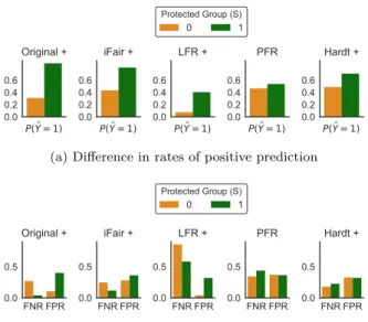
Group Fairness: However, PFR clearly outperforms all other methods on group fairness. It achieves near-equal rates of positive predictions as shown in Figure 9a, and near-equal error rates across groups as shown in Figure 9b. Again, PFR’s performance on group fairness is as good as that of Hardt which is solely designed for equalizing error rates by post-processing the classifier’s outcomes.
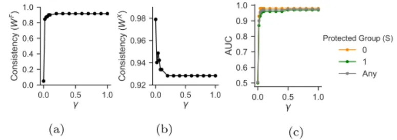
Influence of Hyper-Parameterγ: Figures 10a and 10b show the same effects as observed for the other datasets: increasingγhelps consistency w.r.t. WF and degrades con-sistency w.r.t. WX. Likewise, Figure 10c confirms that higherγhurts AUC over both groups together. However, as before,AUC for the protected group (S =1) improves and
the gap in AUC between the two groups decreases when
P(Y = 1) 0.0 0.2 0.4 0.6 Original + P(Y = 1) 0.0 0.2 0.4 0.6 iFair + P(Y = 1) 0.0 0.2 0.4 0.6 LFR + P(Y = 1) 0.0 0.2 0.4 0.6 PFR P(Y = 1) 0.0 0.2 0.4 0.6 Hardt + Protected Group (S) 0 1
(a) Difference in rates of positive prediction
FNR FPR 0.0 0.5 Original + FNR FPR 0.0 0.5 iFair + FNR FPR 0.0 0.5 LFR + FNR FPR 0.0 0.5 PFR FNR FPR 0.0 0.5 Hardt + Protected Group (S) 0 1
(b) Difference in error rates (FPR and FNR)
Figure 9: Compas Data: Difference between Groups in (a) Rate of Positive Predictions and (b) Error Rates.
γ is set higher. So the PFR way of incorporating pairwise judgements helps the protected group.
0.0 0.5 1.0 0.525 0.550 0.575 0.600 0.625 Consistency ( W F) Compas (a) 0.0 0.5 1.0 0.80 0.85 0.90 0.95 Consistency ( W X) Compas (b) 0.0 0.2 0.4 0.6 0.8 1.0 0.60 0.65 AUC Protected Group (S) 0 1 Any (c) Figure 10: Influence of γ on (a) Individual Fairness w.r.t.
WF (b) Individual Fairness w.r.t. WX and (c) Utility
4.4
Discussion and Lessons
PFRoutperforms all other methods on individual fairness regardingWF for an acceptable performance in AUC, even when these baselines are given the same side-information for their augmented version (suffixed +). The improvement in individual fairness in WF comes at the expense of reduc-ing individual fairness forWX, an unavoidable trade-off if the two views of fairness – data attributes (WX) and pair-wise judgements (WF) – exhibit inherent tension. As for group fairness,PFR clearly outperforms all other represen-tation learning methods, with group-fairness metrics as good as those of Hardt whose sole optimization goal is to equal-ize the error rates. This strong behavior of PFR on group fairness measures is remarkable as PFR is not explicitly de-signed for this goal. It underlines, however, the point that pairwise judgements is highly beneficial side-information, es-pecially when comparing individuals from a-priori incompa-rable groups via quantiles from within-group rankings. The flexibility to incorporate such information is a salient advan-tage of PFR, missing in prior works for fair representation learning.
5.
CONCLUSIONS
This paper proposes a new departure for the hot topic of how to incorporate fairness in algorithmic decision mak-ing. Building on the paradigm of individual fairness, we devised a new method, calledPFR, for operationalizing this line of models, by eliciting and leveraging side-information on pairs of individuals who are equally deserving and, thus, should be treated similarly for a given task. We developed an optimization model to learn Pairwise Fair Representa-tions (PFR), using the fairness graphs of pairwise judge-ments as inputs. We carried out comprehensive experijudge-ments with the Compas recidivism data and decile scores derived from questionnaires, and with the Crime & Communities data on socio-economic properties and ratings of neighbor-hoods by former and current residents. In both cases, the side-information on fairness turned out to be beneficial for giving members of the protected group their deserved share, resulting in high individual fairness and high group fairness (near-equal error rates across groups), with reasonably low loss in utility.
6.
REFERENCES
[1] E. Amid and A. Ukkonen. Multiview triplet
embedding: Learning attributes in multiple maps. In ICML, 2015.
[2] E. Anderson, Z. Bai, J. Dongarra, A. Greenbaum, A. McKenney, J. Du Croz, S. Hammarling,
J. Demmel, C. Bischof, and D. Sorensen. Lapack: A portable linear algebra library for high-performance computers. InICS, 1990.
[3] J. Angwin, J. Larson, S. Mattu, and L. Kirchner. Machine bias: There’s software used across the country to predict future criminals and it’s biased against blacks.In ProPublica 2016.
[4] A. Asudeh, H. V. Jagadish, J. Stoyanovich, and G. Das. Designing fair ranking schemes. InSIGMOD, 2019.
[5] J. Biega, K. P. Gummadi, and G. Weikum. Equity of attention: Amortizing individual fairness in rankings. InSIGIR, 2018.
[6] T. Brennan, W. Dieterich, and B. Ehret. Evaluating the predictive validity of the compas risk and needs assessment system.CJB, 2009.
[7] R. L. Brooks.Rethinking the American race problem. Univ of California Press, 1992.
[8] T. Calders, F. Kamiran, and M. Pechenizkiy. Building classifiers with independency constraints. InICDM, 2009.
[9] L. E. Celis, D. Straszak, and N. K. Vishnoi. Ranking with fairness constraints. InICALP, 2018.
[10] F. Chierichetti, R. Kumar, S. Lattanzi, and S. Vassilvitskii. Fair clustering through fairlets. In NIPS, 2017.
[11] A. Chouldechova. Fair prediction with disparate impact: A study of bias in recidivism prediction instruments.Big data, 2017.
[12] S. Corbett-Davies, E. Pierson, A. Feller, S. Goel, and A. Huq. Algorithmic decision making and the cost of fairness. InKDD, 2017.
[13] K. Crawford. Artificial intelligenceˆa ˘A´Zs white guy problem.The New York Times 2016, 2016. [14] C. Dwork, M. Hardt, T. Pitassi, O. Reingold, and
R. S. Zemel. Fairness through awareness. InITCS, 2012.
[15] S. Elbassuoni, S. Amer-Yahia, C. E. Atie,
A. Ghizzawi, and B. Oualha. Exploring fairness of ranking in online job marketplaces. InEDBT, 2019. [16] M. Feldman, S. A. Friedler, J. Moeller, C. Scheidegger,
and S. Venkatasubramanian. Certifying and removing disparate impact. InKDD, 2015.
[17] S. A. Friedler, C. Scheidegger, and
S. Venkatasubramanian. On the (im)possibility of fairness.CoRR, abs/1609.07236, 2016.
[18] S. Gillen, C. Jung, M. Kearns, and A. Roth. Online learning with an unknown fairness metric. In NeurIPS, 2018.
[19] W. L. Hamilton, R. Ying, and J. Leskovec. Representation learning on graphs: Methods and applications.IEEE Data Eng. Bull., 2017. [20] M. Hardt, E. Price, and N. Srebro. Equality of
opportunity in supervised learning. InIn NIPS 2016. [21] C. Jung, M. Kearns, S. Neel, A. Roth, L. Stapleton,
and Z. S. Wu. Eliciting and enforcing subjective individual fairness.arXiv preprint arXiv:1905.10660, 2019.
[22] M. J. K., J. R. L., C. R., and R. S. Counterfactual fairness. InNIPS, 2017.
[23] F. Kamiran, T. Calders, and M. Pechenizkiy.
Discrimination aware decision tree learning. InICDM, 2010.
[24] T. Kamishima, S. Akaho, H. Asoh, and J. Sakuma. Considerations on fairness-aware data mining. In ICDM, 2012.
[25] T. Kamishima, S. Akaho, and J. Sakuma. Fairness-aware learning through regularization approach. InICDMW, 2011.
[26] M. Kearns, A. Roth, and Z. S. Wu. Meritocratic fairness for cross-population selection. InICML, 2017. [27] J. Kleinberg and E. Tardos. Approximation algorithms
for classification problems with pairwise relationships: Metric labeling and markov random fields.JACM, 2002.
[28] J. M. Kleinberg, S. Mullainathan, and M. Raghavan. Inherent trade-offs in the fair determination of risk scores. InITCS, 2017.
[29] P. Lahoti, K. P. Gummadi, and G. Weikum. ifair: Learning individually fair data representations for algorithmic decision making. InICDE, 2019. [30] Y. Lin, T. Liu, and H. Chen. Semantic manifold
learning for image retrieval. InACM Multimedia, 2005. [31] R. M. Communities and crime dataset, uci machine
learning repository, 2009.
[32] D. Pedreschi, S. Ruggieri, and F. Turini.
Discrimination-aware data mining. InKDD, 2008. [33] B. Salimi, L. Rodriguez, B. Howe, and D. Suciu.
Interventional fairness: Causal database repair for algorithmic fairness. InSIGMOD, 2019.
[34] T. Speicher, H. Heidari, H. Grgic-Hlaca, K. Gummadi, A. Singla, A. Weller, and M. B. Zafar. A unified approach to quantifying algorithmic unfairness: Measuring individual &group unfairness via inequality indices. InKDD, 2018.
set selection with fairness and diversity constraints. In EDBT, 2018.
[36] M. Zafar, I. Valera, M. Rodriguez, K. Gummadi, and A. Weller. From parity to preference-based notions of fairness in classification. InNIPS, 2017.
[37] M. B. Zafar, I. Valera, M. Gomez-Rodriguez, and K. P. Gummadi. Fairness beyond disparate treatment & disparate impact: Learning classification without
disparate mistreatment. InWWW, 2017.
[38] M. B. Zafar, I. Valera, M. Gomez-Rodriguez, and K. P. Gummadi. Fairness constraints: Mechanisms for fair classification. InAISTATS, 2017.
[39] R. S. Zemel, Y. Wu, K. Swersky, T. Pitassi, and C. Dwork. Learning fair representations. InICML, 2013.