Analysis of Multi Attribute Decision Making Problems by Using of Data Envelopment Analysis Technique

Journal of

Applied Research on Industrial Engineering

Journal of Applied Research on Industrial Engineering

Vol. 1, No. 4 (2014) 198-207

Analysis of Multi Attribute Decision Making Problems by Using of Data

Envelopment Analysis Technique

Saeid Nasrollahi-Sebdani

1*1

_{, Majid Esmaelian}

2

_{, Daryush Mohamadi-Zanjirani}

3

1_{Department of Industrial Engineering, Najafabad Branch, Islamic Azad University, Najafabad, Iran ([email protected])} 2 _{Department of Management, Isfahan University, Isfahan, Iran ([email protected])}

3 _{Department of Management, Isfahan University, Isfahan, Iran ([email protected])}

A B S T R A C T A R T I C L E I N F O

Data Envelopment Analysis (DEA) is used for calculating of relative efficiency and then ranking of decision making units (DMU) subject to inputs and outputs in a continuous decision making space. In this paper, DEA models, Cook and Kress Model and Belton-Vickers model have been applied as a multi attribute decision making (MADM) tool and compared analytically to other MADM models such as simple additive weighted (SAW) and technique for order preference by similarity to ideal solution (TOPSIS). For this purpose, after simulating some decision making matrixes and replacing DMU with alternatives, outputs with criteria to be maximized, inputs with criteria to be minimized, alternatives will be ranked by these models. The results of this study show that incorporating decision maker value judgments into the DEA models (restricted DEA models) provide comparable results to traditional MADM models (such as SAW and TOPSIS that are applied more than others). So, restricted DEA models seem to be an advantageous tool for solving MADM problems.

Article history : Received: 15 September 2014 Received in revised format: 2 October 2014

Accepted: 5 October 2014 Available online: 1 December 2014 Keywords:

Data Envelopment Analysis, Multi Attribute Decision Making, Efficiency.

1.

Introduction

The primal aim in DEA is not to rank DMUs; the intention is to recognize ‘efficient’ and ‘inefficient’ DMUs. In MADM, there are some alternatives which are described by some criteria and the decision maker should select one of these alternatives which is ranked higher than others. In fact, DEA measures relative efficiency of each DMU and separates efficient DMUs from inefficient DMUs.

There are some articles on the use of DEA models as an MADM tool. Some researchers represented new models and others tried to compare results of DEA and MADM models. Belton

199

and Vickers (1992) by using of relation between DEA and MADM and also dominance concept

(which is used in MADM models) represented a model to identify dominant alternatives and rank them. Doyle and Green (1993) adjusted Sexton model to prevent from obtaining different weights of outputs and inputs and then applied this adjusted model to solve an MADM problem. Cook and Kress (1994) by definition of composite index and representing a model solved MADM problems with both qualitative and quantitative data. Stewart (1996) compared Belton and Vickers models and performed sensitivity analysis with an applied example. Bouyssou (1999) represented a model which uses convex efficiency concept and also ‘return to scale’ problem is neglected by converting of outputs and inputs to maximizing criteria. Sarkis (2000) compared some basic DEA ranking models with some MADM models by using of an applied example and finally discussed that DEA ranking models can be used to solve MADM problems.

In spite of the fact that some good achievements have been obtained (even some new models) by researchers, they have not found a comprehensive method to solve MADM problems by DEA models (due to some basically differences between two areas) and there are lots of unsolved problems in this case.

2.

Applying DEA as an MADM tool

There are some similarities between DEA and MADM formulations such as inputs and outputs as negative and positive criteria or attributes which suggest using DEA models for solving MADM problems.

3.

Efficiency in DEA and MADM

The relation between ‘efficiency’ concept in DEA and ‘convex efficiency’ in MADM is not new. Suppose that X {a₁,...,a_n} is a finite set of alternatives that have been defined on criteria set. For avoiding ‘return to scale’ problem, all inputs are transformed to outputs. Also

0



y_kj is the value of alternative

a

_k on criterion j. Alternative _{a i} is dominated by alternative

a_kif y_kjy_ij,k 1,...,land at least one of these inequalities is strict. In other words,

alternative a is called efficient alternative in X if other alternatives does not dominate it.

4.

Return to scale

Recognition of ‘return to scale’ is a problem which has not been solved yet. One way to solve this problem is change of minimizing criteria (inputs) to maximizing criteria (outputs) and disregarding return to scale. In fact there is no transformation process of inputs outputs in decision making matrix even in most problems there is not any relation between them.

5.

CCR Model

Charnes, Cooper and Rhodes (1976) represented the first DEA model called CCR which measures relative efficiency of DMUs with several inputs and outputs. Assume that a set of n DMU j (j=1,…,n) using m inputs

x

ij (i=1,…,m) and generating s outputs

y

rj (r=1,…,s).An

200

0

,

,

...

,

2

,

1

0

1

:

1 1 1 1



















   

v

u

n

j

x

v

y

u

x

v

st

y

u

Max

i r ij m i i rj s r r io m i i ro s r r (1)

Where

v

i and

u

r are input and output weights. This basic DEA model does not always

discern and rank DMUs completely, particularly where some of DMUs are efficient and have efficiency value equal to 1.

6.

DEA Ranking Models

Although there are lots of models to rank alternatives which have advantages but also they have some disadvantages. In this paper, models, which have less disadvantages, are preferred.

6.1.

Andersen and Petersen model (a super-efficiency model)

Andersen and Petersen proposed a model (has been shown in model 2) for ranking efficient units which determines the most efficient unit. Measure of Efficient units can be greater than one and these units are ranked like as inefficient units. In this method, at first CCR model should be solved and efficient units are determined then model 2 is solved for each DMU.

0

,

,

,

...

,

2

,

1

0

1

:

1 1 1 1





















   

v

u

o

j

n

j

x

v

y

u

x

v

st

y

u

Max

i r ij m i i rj s r r io m i i ro s r r (2)

There are two problematic issues. First, infeasibility problem, which if it happens, all DMUs are not ranked completely. The second problem is about unstable solutions, which means some efficient DMUs have great efficiency scores.

6.2.

LJK-CCR model (a super-efficiency model)

201

. , ,..., 1 0 , 0 , 0 , 0 ; ,..., 1 ; , ,... 1 : 1 1 2 1 1 2 1 1 1 2 o j n j s s s s r y s y m i x s s x st R s m Min r i i j ro r rj n o j j j io i i ij n o j j j m i _i i                                    







(3)

Where R

 

xij n j i max

1 

_{ . It should be noticed that defining one free variable}

s

i instead of both

slack variables

s

i



1 and si



2 cause to infeasible solutions for dual model.

In optimal solution,

DMU

o, which is DEA efficient in the CCR model, is called

super-efficient in the LJK model if objective value is greater than 1.

6.3.

DEA Multiplier models with restricted weights(Assurance Region

method)

Given the fact that criteria weights are determined by models in DEA, decision maker (DM) preferences are disregarded. That is, a criterion may have larger weight than other criteria and then an alternative, which is less preferable, will have higher rank. To avoid this problem, assurance region (AR) approach can be used. Based on AR method, some constraints (similar to (4) and (5)), which have upper and lower bounds for each criterion weight, are added to DEA multiplier models.

m

i

U

v

v

L

i i

i 1,

,

1

,...,

1 ,

1







(4)

s

r

U

u

u

L

r r

r 1,

,

1

,...,

1 ,

1







(5)

Where

L

1,i

,

U

1,i

,

L

1,r

,

U

1,r are lower and upper bounds on ratios

v

i

v

1

,

u

r

u

1 (ratio of criteria weights).

In general, efficiency scores are reduced by adding these constraints and some DMUs which were efficient may become inefficient.

Although assurance region constraints are nonlinear, they can be transformed to linear constraints (like as (6) and (7)).

m

i

v

U

v

v

L

1,i 1



i



1,i 1

,



1

,...,

(6)

s

r

u

U

u

u

L

1,r 1



r



1,r 1

,



1

,...,

(7)

7.

Cook and Kress model

202

quantitative and qualitative data simultaneously. Cook and Kress (1994) proposed a multi

criteria composite index model which uses DEA procedure to solve MADM problems.

Assume that there are N alternatives with

_k

1 ordinal (qualitative) criteria and

k

2 cardinal

(quantitative) criteria.

a

_k

(

i

)

is measure of alternative i in cardinal criterion k and

W

k is weight

of criterion k that



_iN_

a

_k

(

i

)



1

,

k



CARD

1 and

1

2 1 1





  k k

k

W

k .



is scale parameter which

is determined by model and if it is not used in model, solution may be infeasible. Also

d

_kl

(

i

)

is defined subject to ordinal criteria k (k=1,…,

_k

1) which

d

kl

(

i

)



1

if alternative i is ranked in

lth ordinal position (l=1,…,L) and like

a

_k

(

i

)

,

w

_kl is value of lth ordinal position for ordinal

criterion k.

A composite index is written by,

) ( ) ( 1 i a W x i d W R _k CARD k k kl kl ORD k L l k

i

 





 







(8)

Where _{x kl}_{W kl} kORD and because of data normalizing composite index

R

_i has upper bound 1 for each alternative i.therefore Cook-Kress model is,

(9)

Where Mkl



_iN_1d kl(i) ,kORD.

g

L parameters are bounds on gaps

(

x

kl



x

k(l1)

)

and decision variables

u

_k , which are determined by model, show criteria clearness. In particular, if

criterion

k

1 is clearer than

k

2 , constraint u_k1u_k2 (or u_k u_k z 0

2

1   where z is a positive variable) is added to model.

Below algorithm is used for ranking alternatives,

Step1: preparing data. At first, converting negative criteria to positive criteria and second normalizing weights.

Step2: Model is solved by using specified

g

_l and clarity of criteria and then

R

_i is obtained.

Step3: finally, alternatives are ranked according to

R

_i measures.

203

8.

Bouyssou Model

A ‘folk theory’ in MCDM context says that alternative a_j is efficient if a strict additive

weights of a _j is greater than or equal to other alternatives. a _j is called convex efficient (CE)

and other alternatives are called convex dominated (CD). Convex efficient alternatives are assigned by Bouyssou model,

(10) (10) (10)

Where



is an arbitrarily small positive number,

w

_k is weight of criterion k and

y

_ko is measure of alternative

a

_o according to criterion k and also negative criteria should be

transformed to positive criteria. So

a

_o is convex efficient if D=0. Finally, convex efficient alternatives are ranked higher than convex dominated alternatives.

9.

Belton-Vickers model

Belton and Vickers represented a model based on dominance concept. Suppose that

u

_r and

v

_i are positive and negative criteria weights. x_ij and

y

_rj are measure of alternative a _j

according to negative criterion i (input) and positive criterion r (output). a _j is dominated by

a

_o if r(r=1,…,s) y_roy_rj and i(i=1,…,m) x_ijx_io and at least one of these inequalities being strict. So,

a

_o is ranked higher than a _j . Belton and Vickers model is written by the

following LP model,

(11)

Where  is maximum of deviations _Dj (j=1,…,n).

It should be point out that both Bouyssou and Belton-Vickers models have identical ranking results because the difference between them is only due to changing data.

204

10.

Comparing results of DEA ranking models with MADM models

In this section, discrimination power and correlation of ranking results in DEA models and MADM models are compared by solving some examples. Hence, 15 decision making matrixes with quantitative and qualitative criteria are simulated. Each simulated example has some inputs (minimizing criteria) and some outputs(maximizing data) which one of these outputs has qualitative data. Quantitative data are selected from discrete uniform distribution in range of 1 to 100. For using these data in DEA models, qualitative data should be converted to quantitative data by Likert scale but this process is not used for solving Cook-Kress model. Also Criteria weights are gained by using of Shanon entropy method.

10.1.

Comparing Discrimination Power of Models

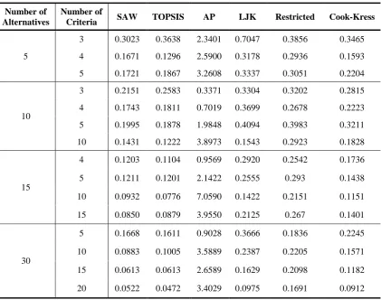
After solving simulated problems by DEA ranking and MADM models and getting their results, standard deviation of results is calculated for comparing of discrimination power of models. It can be deduced that models with greater standard deviation value have more discrimination power. Greater standard deviation value means alternatives ranking is easier but when results are very close, ranking validity is doubtful. Table 1 and chart 1 have showed this result.

Table 1 standard deviations of models results

Number of Alternatives

Number of

Criteria SAW TOPSIS AP LJK Restricted Cook-Kress

5

3 0.3023 0.3638 2.3401 0.7047 0.3856 0.3465

4 0.1671 0.1296 2.5900 0.3178 0.2936 0.1593

5 0.1721 0.1867 3.2608 0.3337 0.3051 0.2204

10

3 0.2151 0.2583 0.3371 0.3304 0.3202 0.2815

4 0.1743 0.1811 0.7019 0.3699 0.2678 0.2223

5 0.1995 0.1878 1.9848 0.4094 0.3983 0.3211

10 0.1431 0.1222 3.8973 0.1543 0.2923 0.1828

15

4 0.1203 0.1104 0.9569 0.2920 0.2542 0.1736

5 0.1211 0.1201 2.1422 0.2555 0.293 0.1438

10 0.0932 0.0776 7.0590 0.1422 0.2151 0.1151

15 0.0850 0.0879 3.9550 0.2125 0.267 0.1401

30

5 0.1668 0.1611 0.9028 0.3666 0.1836 0.2245

10 0.0883 0.1005 3.5889 0.2387 0.2205 0.1571

15 0.0613 0.0613 2.6589 0.1629 0.2098 0.1182

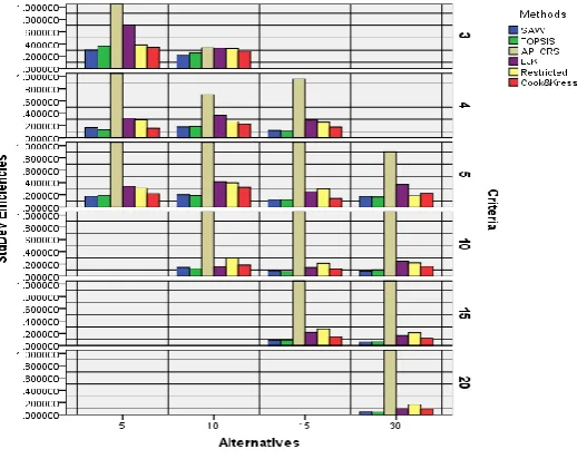
205

Fig 1. Bar charts of standard deviations

Considering table 1 and figure 1, DEA ranking models and also Cook-Kress model have greater standard deviation than SAW and TOPSIS models. In fact, results of SAW and TOPSIS models are closer to each other than DEA ranking models, especially in big problems. So, it can be concluded that results with smaller standard deviations are closer to each other and have less discrimination power. For example in problem with 15 alternatives and 15 criteria, standard deviations of SAW and TOPSIS results (0.09 approximately) are smaller than DEA ranking results.

Also due to identical results of Bouyssou and Belton-Vickers models and also existence of so many convex efficient alternatives (which have zero value) in big problems, the results have not been expressed.

10.2.

Comparing Correlation Coefficients Between Models

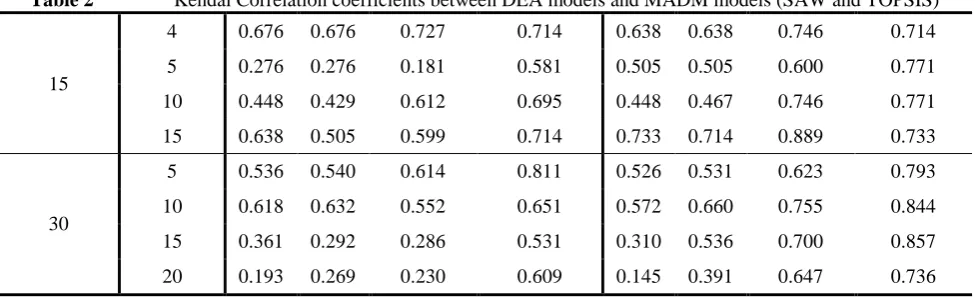
It should be explained that the ranking orders are not exactly the same between DEA ranking models and MADM models. Kendal correlation coefficient is used to calculate correlations between DEA models and MADM models and determine how well the ordinal ranks of all models correlated with each other. The results are shown on table 2.

Table 2 Kendal Correlation coefficients between DEA models and MADM models (SAW and TOPSIS)

SAW TOPSIS

Number of Alternatives

Number of

Criteria AP LJK Restricted Cook-Kress AP LJK Restricted

Cook-Kress

5

3 0.8 0.8 0.8 0.8 0.8 0.8 0.8 0.8

4 0.4 0.4 0.8 0.6 0.2 0.2 0.6 0.4

5 1 1 0.8 0.8 0.8 0.8 1 1

10

3 0.689 0.689 0.822 0.778 0.511 0.511 0.644 0.867

4 0.733 0.689 0.733 0.6 0.689 0.733 0.778 0.911

5 0.689 0.689 0.822 0.511 0.822 0.822 0.956 0.556

206

Table 2 Kendal Correlation coefficients between DEA models and MADM models (SAW and TOPSIS)

15

4 0.676 0.676 0.727 0.714 0.638 0.638 0.746 0.714

5 0.276 0.276 0.181 0.581 0.505 0.505 0.600 0.771

10 0.448 0.429 0.612 0.695 0.448 0.467 0.746 0.771

15 0.638 0.505 0.599 0.714 0.733 0.714 0.889 0.733

30

5 0.536 0.540 0.614 0.811 0.526 0.531 0.623 0.793

10 0.618 0.632 0.552 0.651 0.572 0.660 0.755 0.844

15 0.361 0.292 0.286 0.531 0.310 0.536 0.700 0.857

20 0.193 0.269 0.230 0.609 0.145 0.391 0.647 0.736

It can be inferred from table 2 that DEA models with restriction weights and Cook-Kress model have greater correlation values with MADM models than other DEA models. Indeed, the rankings of DEA models with restriction weights seem to correlate well with both SAW and TOPSIS models.

11.

Discussion and Conclusions

According to DEA literature, DEA models are categorized into two kinds of models, constant returns to scale (CRS) and variable returns to scale (VRS). In case of VRS against CRS, results of input-oriented models are different from output-oriented models. So, it should be noticed that CCR model and ranking DEA models which apply CRS concept, must be used instead of BCC model. This point has been followed by researchers and they have used CCR model to compare with MADM models in their articles.

In this research, results of DEA and MADM models were compared by solving simulated examples. Although, the recognition of which MADM methods are the best has been a difficult goal to be obtained by researchers, SAW and TOPSIS methods which are used more than other methods are applied and compared with DEA ranking models.

In conclusion, DEA ranking models (such as AP, LJK and models with restriction weights) and Cook-Kress model (which uses both quantitative and qualitative criteria) have more discrimination power than MADM models (SAW and TOPSIS) especially in big problems. MADM models are so close compare to DEA models and eventually valid ranking of alternatives is questionable. Another important point should be expressed that there is no generally accepted method to make a relative comparison of DEA models or any other MADM models among themselves. However, comparing of ranking results has been performed by determining of Kendal correlation coefficient and finally results of DEA models and Cook-Kress model have good correlation with MADM models. So these models can be used to solve MADM problems. In addition to this, models with restriction weights because of applying value judgments are the best choice for solving MADM problems. In other words, incorporating decision maker or manager preferences enhances the correlation between DEA and MADM models.

207

12.

Acknowledgments and Legal Responsibility

The authors are also grateful to Dr. H. Shirouyehzad for his guidance to complete this paper.

13.

References

Adler, N, Friedman, L and Sinuany-Stern, Z (2002) “Review of ranking methods in the data envelopment analysis context “, European Journal of Operational Research , Vol. 140, pp. 249-265.

Belton, V and Vickers, S.P (1992) “ VIDEA: integrated DEA and MCDA- A visual interactive approach “ , Proceedings of the Tenth International Conference on Multiple

Criteria Decision Making , Vol. 2, pp. 419-429.

Bouyssou, D. (1999)”Using DEA as a tool for MCDM : some remarks” , Journal of the

Operational Research Society,Vol. 50, pp. 974-978.

Cook, W.D and kress, M.(1994) “A multiple-criteria composite index model for quantitative and qualitative data “, European Journal of Operational Research, Vol. 78, pp. 367-379.

Cook, W.D and Seiford, L.M. (2009),”Data envelopment analysis (DEA) – Thirty years on”,

European Journal of Operational Research, Vol. 192, pp. 1-17.

Cooper, W.W, Seiford, L.M and Tone, K.(2006) Introduction To Data Envelopment Analysis and Its Uses , USA , NY : Springer.

Doyle, JR and Green, R.H.(1993)”Data Envelopment Analysis and Multiple Criteria Decision Making”, OMEGA, Vol. 21, No. 6, pp. 713-715.

Ishizaka, A and Nemery, P, (2013) Multi-Criteria Decision Analysis – Methods and

Software , United Kingdom, John Wiley & Sons.

Sarkis,J,(2000)”A comparative analysis of DEA as a discrete alternative multiple criteria decision tool”, European Journal of Operational Research, Vol. 123, pp. 543-557.

Stewart, t.(1996)”Relationships between Data Envelopment Analysis and Multi criteria Decision Analysis ”, Journal of the Operational Research Society,Vol. 47, pp. 654-665.

Shanling, LI , Jahanshahloo, G.R and Khodabakhshi, M.(2007)” A super-efficiency model for ranking efficient units in data envelopment analysis”, Applied Mathematics and

Computation, Vol. 184, pp. 638–648.

Venkata Rao, R. (2013) Decision Making in the Manufacturing Environment Using Graph

Theory and Fuzzy Multiple Attribute Decision Making Methods, USA, NY: Springer