1
Spatio-temporal downscaling of gridded crop model yield estimates based on
1
machine learning
2
C. Folbertha, A. Baklanovb,c, J. Balkoviča,d, R. Skalskýa,e, N. Khabarova, M. Obersteinera 3
4
a International Institute for Applied Systems Analysis, Ecosystem Services and Management Program, Schlossplatz
5
1, A-2361 Laxenburg, Austria, [email protected], [email protected], [email protected], 6
[email protected], [email protected] 7
b International Institute for Applied Systems Analysis, Advanced Systems Analysis Program, Schlossplatz 1, A-2361
8
Laxenburg, Austria, [email protected] 9
c National Research University Higher School of Economics, Soyuza Pechatnikov str., 16, St. Petersburg, Russian
10
Federation 11
d Department of Soil Science, Faculty of Natural Sciences, Comenius University in Bratislava, Ilkovičova 6, 842 15
12
Bratislava, Slovak Republic, [email protected] 13
e National Agricultural and Food Centre, Soil Science and Conservation Research Institute, Trencianska 55, 824 80
14
Bratislava, Slovak Republic, [email protected] 15 16 Corresponding author: 17 Christian Folberth 18 Schlossplatz 1 19
A-2361 Laxenburg, Austria 20
E-Mail address: [email protected] 21
2 Highlights:
22
Machine learning allows for highly accurate downscaling of GGCM outputs 23
Increasing detail of climate features improves prediction accuracy 24
Feature importance ranks in the order climate ≥ cultivar > soil and topography 25
Approach is scale-free and does not require prior assumptions on feature importance 26
It enables the development of robust downscaling tools with low user bias 27
3 Abstract
29
Global gridded crop models (GGCMs) are essential tools for estimating agricultural crop yields 30
and externalities at large scales, typically at coarse spatial resolutions. Higher resolution 31
estimates are required for robust agricultural assessments at regional and local scales, where the 32
applicability of GGCMs is often limited by low data availability and high computational 33
demand. An approach to bridge this gap is the application of meta-models trained on GGCM 34
output data to covariates of high spatial resolution. In this study, we explore two machine 35
learning approaches – extreme gradient boosting and random forests - to develop meta-models 36
for the prediction of crop model outputs at fine spatial resolutions. Machine learning algorithms 37
are trained on global scale maize simulations of a GGCM and exemplary applied to the extent of 38
Mexico at a finer spatial resolution. Results show very high accuracy with R2>0.96 for 39
predictions of maize yields as well as the hydrologic externalities evapotranspiration and crop 40
available water with also low mean bias in all cases. While limited sets of covariates such as 41
annual climate data alone provide satisfactory results already, a comprehensive set of predictors 42
covering annual, growing season, and monthly climate data is required to obtain high 43
performance in reproducing climate-driven inter-annual crop yield variability. The findings 44
presented herein provide a first proof of concept that machine learning methods are highly 45
suitable for building crop meta-models for spatio-temporal downscaling and indicate potential 46
for further developments towards scalable crop model emulators. 47
Keywords: meta-model, extreme gradient boosting, random forests, maize yield, agricultural 48
externalities, climate features 49
4 1Introduction
50
In recent years, global gridded crop models (GGCMs) - combinations of a crop model 51
and global sets of gridded data - have become essential tools for estimating crop yields and 52
agricultural externalities under a wide range of environmental and management conditions (e.g. 53
Müller et al., 2017). Besides the direct provision and interpretation of model outputs for crop 54
yields alone (e.g. Rosenzweig et al., 2014) or their joint evaluation with externalities such as 55
crop water use (Liu et al., 2013; Elliott et al., 2014), GGCMs provide base layers of input data 56
for agro-economic or integrated assessment models (IAMs; Müller and Nelson, 2014) e.g. for 57
land use change analyses and optimization (e.g. Havlík et al., 2011). 58
The present global standard resolution of input data is 0.5° x 0.5° corresponding to 59
approx. 50 km x 50 km near the equator. This is foremost determined by climate data, which are 60
rarely available at higher resolutions at a global scale. Further common input data are 61
management information and in most cases soil data and topography (Müller et al., 2017). The 62
latter two are available at increasingly fine resolutions well below 1 km (Hengl et al., 2017a, 63
Jarvis et al., 2008), while management is typically reported at national or subnational 64
administrative levels (e.g. Sacks et al., 2010; Mueller et al., 2012). In few cases, simulations are 65
run at the sub-grid level accounting for some heterogeneity in soil and topography (Skalský et 66
al., 2008; Balkovič et al., 2014). Regardless of the spatial resolution, each simulation unit is 67
treated as a homogenous field in the crop model. 68
While this spatial resolution provides sufficient detail for robust assessments at macro 69
scales such as the country level, there is increasing concern that GGCM estimates and hence 70
impact assessments at coarse resolutions often miss actual on-ground conditions. As only 71
5
average or dominant characteristics present within each grid are considered for simulations, 72
assumptions and data may not match actually farmed land (e.g. Folberth et al., 2016) and 73
farming practices (e.g. Reidsma et al., 2009). In addition, they may omit farm-level 74
heterogeneity present at the sub-grid level (Ewert et al., 2011), which is essential for local to 75
regional decision-making and stakeholder information (Rosenzweig et al., 2018). 76
Applying gridded crop models at very high spatial resolutions on the other hand increases 77
computational demand substantially and is often limited by data availability as outlined above. 78
Foremost climate data at suitable temporal resolutions for crop models - which is typically a 79
daily time step (Müller et al., 2017) - are hardly available at fine spatial resolutions. The 80
presently highest resolving global daily dataset known to the authors has 0.25° x 0.25° (Ruane et 81
al., 2015), while regional products may have resolutions of up to 0.11° x 0.11° (Haylock et al., 82
2008). Temporally coarser data e.g. with a monthly time step, however, are available at very fine 83
resolutions up to <1 km (e.g. Wang et al., 2016; Fick and Hijmans, 2017). 84
An approach lending itself to address these issues in an efficient and flexible way is the 85
use of meta-models built from coarser GGCM simulations. This allows for deriving estimates of 86
crop yields and associated agricultural externalities at high, virtually scale-free, spatial 87
resolutions without requirements for setting up high-resolution crop model infrastructures 88
including their comprehensive data requirements. There is no scientific literature on crop meta-89
model development for spatio-temporal predictions across scales known to the authors. The 90
potentially most closely related field is the recently evolving crop model emulator development 91
at the grid cell level. Examples are the development of regressions along climate change 92
trajectories as such (e.g. Blanc and Sultan, 2015; Blanc, 2017) or the use of global crop model 93
6
simulations with artificial alterations of climate variables to retrieve estimates of climate change 94
impacts for assessment studies based on regressions along temperature, precipitation, and CO2
95
concentrations (Ruane et al., 2017; Rosenzweig et al., 2018). The production of high-resolution 96
crop yield surfaces in contrast is foremost accomplished using simplified crop model algorithms 97
(e.g. IIASA/FAO, 2012) or purely statistical approaches (e.g. Mueller et al., 2012). Common to 98
all referenced approaches is that they (a) are based on narrow sets of a priori selected covariates 99
based on modelers’ assumptions and (b) do not allow for or have not been tested for the joint 100
evaluation of agricultural productivity and externalities. Crop model emulators are in addition 101
typically parameterized at the grid level, which renders them spatially determined and scale-102
depended. 103
The presently most flexible approaches for data-driven development of models with high 104
accuracy can be found in the field of machine learning. Machine learning is a collective term for 105
a wide range of data analysis and data-driven forecasting techniques. The most advanced 106
techniques are characterized by the ability to digest large amounts of covariates (herein syn.
107
features, syn. predictors) to provide predictions for both numeric and categorical variables with 108
algorithms of high complexity and flexibility, which determine the relevance of provided 109
covariates themselves (e.g. Witten et al., 2016). Examples of methodologic approaches are 110
neural networks, various forms and derivatives of regression trees, as well as clustering 111
techniques. While simpler methods such as multiple linear or lasso regressions are typically 112
computationally faster and straightforward to interpret, they show typically a substantially lower 113
performance. Within agricultural sciences, applications are to date mostly limited to processing 114
and analyzes of remote sensing data (e.g. Duro et al., 2012; Ali et al., 2015). Few exceptions are 115
7
the development of crop nutrient response models for studying yield responses in sub-Saharan 116
Africa based on field trial data (Hengl et al., 2017b) and the use of data mining tools for 117
identifying crop growth limitations (Delerce et al., 2016). 118
119
120
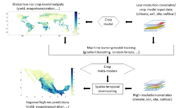
Figure 1. Schematic representation of the downscaling approach presented in this study. 121
Machine-learning derived meta-models trained on global crop model outputs and 122
covariates at a comparably low spatial resolution are used for producing regional 123
estimates of corresponding variables at a higher spatial resolution. 124
In this study, we evaluate machine learning as an approach for building crop meta-125
models. The focus is on the feasibility to use low-resolution global crop simulations of maize 126
yield potential for predictions at a high resolution, here exemplary the extent of Mexico, as 127
8
depicted schematically in Figure 1. Non-nutrient and pest limited yield potentials (Lobell et al., 128
2009) with and without sufficient water supply were selected as a target variable as they allow 129
for a thorough evaluation of climate-related covariates without inference from soil nutrient 130
trajectories. Two of the presently most flexible and in recent competitions best performing 131
(Fernández-Delgado, 2014; Chen and Guestrin, 2016) machine learning approaches for numeric 132
predictions, extreme gradient boosting and random forests, are tested and compared against crop 133
model simulations carried out at the finer resolution. Objectives of the study are to (a) evaluate 134
the meta-model performance in downscaling the low-resolution global yield simulation to high-135
resolution predictions in the study region of Mexico, (b) identify most important covariates 136
required by the meta-model, and (c) test the approach for predictions of selected agricultural 137
externalities across scales. To provide an exemplary application case, machine learning model 138
predictions are performed at a very high spatial resolution (1 km x 1 km) in major producing 139
areas and benchmarked against reported inter-annual yield variability, a key performance 140
indicator for climate change impact assessments (Müller et al., 2017). Finally, an outlook 141
provides suggestions for further steps to extend the models’ capabilities. 142
2Methods and Data 143
2.1Gridded crop model description 144
Crop simulations were carried out using a gridded version of the Environmental Policy 145
Integrated Climate model (EPIC). EPIC was initially developed to assess the impacts of 146
management on crop yields (Williams, 1995). It has constantly been updated to cover additional 147
processes such as effects of elevated atmospheric CO2 concentration on plant growth (Stockle et
9
al., 1992), detailed soil organic matter cycling (Izaurralde et al., 2006, Izaurralde et al., 2012), 149
and an extended number of crop types and cultivars (e.g. Kiniry et al., 1995; Gaiser et al., 2010) 150
among others (see Gassman, 2004). More details of the crop growth model are provided in 151
Supplementary Text S1. 152
The gridded version of EPIC used here, EPIC-IIASA (Balkovič et al., 2014), runs the 153
EPIC model for a given set of simulation units derived from intersecting homogenous response 154
units (soil and topography), administrative borders, and climate grids (Skalský et al., 2008). 155
Thereby, each simulation unit is treated as a representative, homogenous field. 156
2.2Study regions, delineation of simulation units, and simulation period 157
Simulations and meta-model predictions were performed (a) at the global scale at a 158
coarse spatial resolution and (b) for Mexico at a finer resolution. The latter was selected as an 159
exemplary study region as it encompasses the three major climates tropic, temperate, and (semi-160
)arid and has a large coverage of maize harvest areas. The basic spatial resolutions at the two 161
scales were grids of 5’ (global) and 0.5’ (Mexico), respectively, serving also as basic references 162
for spatial harmonization of all underlying input data (topography, soil, and land cover). 163
Individual pixels were aggregated to homogeneous response units (HRUs) based on slope, 164
altitude and soil classes. HRU provide aggregated spatial units which are expected to be 165
homogenous in their physical response and relatively stable over time. The basic bio-166
physical drivers assumed for an HRU are hardly adjustable by farmers, which allows for 167
analyzing impacts of the same management practices employed across a variety of natural 168
conditions. Intersecting HRUs with administrative units (countries globally and states for 169
10
Mexico) and the climate grids of 0.5° x 0.5° and 0.25° x 0.25° resolution at the global and 170
Mexican scale, respectively, resulted in final simulation units with a total number of 1.3 x 10⁵
171
globally and 2.3 x 10⁵ for Mexico. Spatially explicit inputs for EPIC on topography and soil were 172
then calculated as mean (altitude) or majority (slope, soil) values across all pixels within the 173
simulation unit. Additional evaluations were carried out for the Mexican state of Jalisco, which is 174
the top rainfed maize producing state in the country according to Servicio the Información 175
Agroalimentaria y Pesquera (SIAP, 2018b). 176
Simulations were performed for the years 1980-2010 based on climate data coverage 177
(Section 2.3.1) and evaluated for the period 1990-2009 as the crop model equilibrates during the 178
first simulation years and the global simulations used for training machine learning models did 179
not provide outputs for the year 2010 in regions with growing seasons crossing years. 180
2.3Crop model input data 181
2.3.1 Climate data 182
Gridded climate data were obtained from the publicly available AgMERRA climate 183
dataset (Ruane et al., 2015) at spatial resolutions of 0.5° x 0.5° for global simulations and 184
predictions and 0.25° x 0.25° for the study region of Mexico. AgMERRA covers the period 185
1980-2010 and combines data from the Modern-Era Retrospective Analysis for Research and 186
Applications (MERRA; Rienecker et al., 2011), station data, and remotely sensed datasets and 187
has been bias corrected using stations from agricultural land only. The high-resolution version 188
was obtained from the providers’ website directly, the coarser resolution was provided through 189
the Global Gridded Crop Model Intercomparison (GGCMI) project (Elliott et al., 2015). 190
11
Although higher resolution monthly climate data would be available for the study region (e.g. 191
Wang et al., 2016) allowing for higher resolution meta-model predictions, these would not allow 192
for benchmarking against EPIC simulations requiring daily climate data. 193
2.3.2 Soil data 194
Soil data were retrieved from the Harmonized World Soil Database v1.2 (HWSD; 195
FAO/IIASA/ISRIC/ISS-CAS/JRC, 2012) at both spatial scales. For each grid cell at 5’ (global) 196
or 0.5’ (Mexico) resolution, the dominant soil type of the largest soil mapping unit was selected 197
as the representative soil type. Soil characteristics considered in EPIC and the machine learning 198
approaches are depth, texture, coarse fragment content, bulk density, soil organic carbon content, 199
pH, electric conductivity, cation exchange capacity, base saturation, and carbonate content 200
(Table 1). 201
2.3.3 Topography 202
For the global setup, elevation data were adopted from GTOPO30 (USGS, 2002) 203
calculating the mean elevation in each simulation unit. Slope classes were obtained from the 204
Global Agro-ecological Zones Assessment for Agriculture (GAEZ; Fischer et al., 2012). For the 205
high-resolution setup constructed for Mexico, both elevation and slopes were derived from the 206
SRTM 4.1 database provided by CIAT-CSI (Jarvis et al., 2008). 207
2.3.4 Land use 208
Global low-resolution simulations were carried out for all simulation units presently 209
containing cropland according to at least one of the datasets Global Land Cover 2000 database 210
12
(Global Land Cover 2000 database, 2003) or SPAM (You et al., 2017). For Mexico, simulations 211
were done for all simulation units and MIRCA2000 was used for identifying simulation units 212
containing relevant maize harvest area, here defined as >5% of total area. Selected analyses were 213
restricted to these in order to evaluate model performance for the whole land and relevant 214
cropland only. 215
2.3.5 Crop management 216
Maize was used as a model crop due to its extensive cultivation globally and in Mexico. 217
Default crop parameters from the EPIC model were used, which reflect a high-yielding variety 218
adapted to warm climate (Kiniry et al., 1995). Crop growing seasons were adopted at both scales 219
from Sacks et al. (2010) as provided by Elliott et al. (2015). PHU were calculated from planting 220
to harvest using long-term monthly climate data for the whole time-period covered by the 221
AgMERRA climate dataset (1980-2010) at each spatial resolution separately. 222
To obtain non-nutrient limited maize yield potentials (Lobell et al., 2009), mineral N 223
fertilizer was applied automatically by the EPIC model based on plant stress to avoid plant 224
growth limitations due to nutrient deficits, which may cause trends in yields over time due to 225
nutrient mining. The maximum applied amount of fertilizer was set to 500 kg N ha-1 yr-1, which 226
is commonly more than sufficient for maximizing maize yields (e.g. Folberth et al., 2013). 227
Simulations were carried out with water supply either from precipitation only (rainfed) or with 228
sufficient supplementary irrigation water supply (fully irrigated). Irrigation water was applied 229
based on plant stress analogously to fertilizer with an annual maximum volume of 2000 mm. 230
13
Other management practices were kept at a basic level with four operations in each season: field 231
cultivation, planting, harvest, and stover removal. 232
2.4Machine learning framework 233
We test two state-of-the-art tree-based ensemble methods, extreme gradient boosting and 234
random forests. Ensemble methods employ a collection of learning algorithms to achieve better 235
predictive power than could be gained from any of these algorithms alone. For ensembles such as 236
extreme gradient boosting and random forests, it is typical to use trees as building blocks to
237
allow for invariance to scaling of inputs and complex interactions between features. Since 238
ensembles have additional parameters responsible for aggregation of learning algorithms, they 239
have more flexibility in fitting training data than single-algorithm approaches do. Thus, 240
ensembles are more prone to overfitting. Overfitting is prevented through out-of-bag error 241
monitoring, n-fold cross-validation, correction of the ensemble by regularization that makes the 242
training procedure more conservative, and testing on the holdout dataset covering 25% of 243
observations (see below). Both extreme gradient boosting and random forests are insensitive to 244
multiple correlation of covariates with respect to prediction accuracy and overfitting. The 245
quantification of variable importance, however, may be affected if covariates are strongly 246
correlated (see Section 2.4.3). 247
Crop model simulation data (serving here as observations) for building machine learning 248
models was randomly split into training and validation sets containing 75% and 25% of samples, 249
respectively, which is a common split ratio in machine learning. About 19.5 x 10⁵ samples 250
(simulation units x simulation years) were used for model training and 6.5 x 10⁵ for validation. 251
14
Machine learning models were built separately for the two water management scenarios, rainfed 252
or sufficiently irrigated, within the statistical computing software R (R Development Core Team, 253
2008) using the packages specified in the following sections. 254
To streamline the presentation of results, the main body of the paper focuses on results 255
from extreme gradient boosting. The evaluation of the random forests models is presented in the 256
SI and discussed within the main body where relevant. 257
2.4.1 Extreme gradient boosting 258
Similar to other boosting methods, extreme gradient boosting is an ensemble learning 259
technique that sequentially builds the model: each tree is fit on a modified version of the original 260
training data set. I.e., every new tree uses information from previously grown trees. This is the 261
key difference to random forests (see below). Extreme gradient boosting generalizes boosting 262
methods by allowing minimization of an arbitrary differentiable loss function. In this study, we 263
employed the R package XGBoost for extreme gradient boosting, a highly efficient realization of 264
the gradient boosting approach that showed the best performance in recent machine learning 265
challenges (Chen and Guestrin, 2016). Being a learning algorithm with high flexibility, extreme 266
gradient boosting is prone to overfitting, especially, if training data are scarce, which is not the 267
case here. Typically, parameter tuning is done by performing an exhaustive grid search along 268
parameter dimensions using the default parameters as the reference point. This was here not 269
considered meaningful due to the vast amount of training data, rendering a full grid search 270
computationally inefficient and unneeded, due to extremely low error obtained already in a 271
limited grid search. I.e., we tuned only key parameters for shrinkage and learning (eta, 272
15
max_depth, nrounds; Table S1). In our case, the default parameter values resulted in stable but 273
improvable performance with R2=0.94 for the test dataset. This suggested to increase the
274
maximum tree depth and local variation of the learning rate (eta). The grid search resulted in 275
R2=0.99 for both training and test data with eta=0.15 or 0.30 and max_depth=15 or 20. The 276
lowest RMSE in both training and test data was obtained with eta=0.15 and max_depth=20 in a 277
five-fold cross validation (Table S2). Although this parameter set results in a marginal overfit, it 278
also showed the best performance in regression metrics and mean absolute error (MAE; not 279
shown), the main performance indicators used herein (see section 2.5.1). It was hence selected 280
for performing the predictions. Extending the grid search to by increasing the rounds of tree 281
building (nrounds) from 60 to 100 provided only a negligible increase in performance (Table 282
S2). Resulting parameters were hence eta=0.15, max_depth=20, and – to ensure very high 283
accuracy - nrounds=100. 284
Since extreme gradient boosting may produce negative predictions even if the training 285
data does not have them, the lower boundary was set to zero and all predictions below corrected 286
to this value. This was the case for rainfed crop yields in 0.1% of samples with predictions of up 287
to -0.19 t ha-1 in the validation set and 0.02% of the predictions for Mexico with up to -0.08 t ha -288
1. Irrigated crop yield predictions were affected in the validation set only with up to -0.09 t ha-1 in
289
<0.01% of samples. 290
2.4.2 Random forests 291
In contrast to boosting methods, tree ensembles build a number of models in parallel 292
from which average predictions are derived. Bagging is a basic approach to introduce an 293
16
ensemble that consists of a number of decision trees trained on random subsets of data 294
(bootstrapped training samples). Random forests (Breiman, 2001) employ not only bagging (row 295
sub-sampling) but also column sub-sampling, i.e., every time a split in a tree is examined for a 296
random subset of candidate features drawn from the full set of features. This effectively de-297
correlates the trees. As reported in a recent meta-study of machine learning algorithms 298
(Fernández-Delgado, 2014), random forests was identified as the best family of classifiers. In 299
this study, random forests models were constructed using the R package h2o, which serves as a 300
link to the H2O.ai machine learning cluster environment (The H2O.ai team, 2017). 301
As random forests are less prone to overfitting, global parameters were tuned to achieve a 302
reasonable balance between performance and computational demand, which increases linearly 303
with number of trees and tree depth. Major parameters to adjust in random forest are number of 304
trees (ntrees), maximum tree depth (max_depth), and a number of features considered for each 305
split decision (mtries). The latter is per default one third of total features for numeric predictions. 306
Starting from the default values ntree=50, max_depth=20, and mtries=[number of features]*0.3, 307
we found an increase in performance in terms of regression coefficients and MAE of the test 308
dataset up to max_depth=30 with negligible improvements if ntree was increased from 50 to 80 309
(Figure S1). Further increasing the parameter values provides a marginal increase, but would not 310
justify the increase in computational demand, which is already at any point substantially higher 311
than for extreme gradient boosting (see also section 4.4). Increasing or decreasing the parameter 312
mtries from about 33% of feature number as a default to 20% or 50% affected model 313
performance only marginally as well with no changes in R2 or slope and changes by ±0.01 t ha-1 314
in intercept and MAE. 315
17 2.4.3 Feature importance
316
Both methods determine feature importance internally. To obtain an overall summary of 317
the importance of predictors, the residual sum of squares (for regression) or the Gini index (for 318
classification; Breiman et al. 1984) are used. For ensembles of regression trees, the total amount 319
by which the residual sum of squares is decreased by splits over a fixed feature is calculated and 320
then average over all trees. Larger values point to predictors that are more important. Likewise, 321
in the case of ensembles of classification trees, the total amount that the Gini index is reduced 322
due to splits is cumulated over a given feature and averaged over all trees. For both machine 323
learning methods, we present the relative importance of each feature as percentage. Due to 324
differences in the estimation of feature importance, it is not feasible to compare importance 325
across different algorithms quantitatively. In addition, multiple correlated features, which can be 326
expected here at least among soil characteristics or (monthly) climate variables, are known to 327
bias the quantification of feature importance (Toloşi and Lengauer, 2011). E.g., if two features 328
included in an extreme gradient boosting model are perfectly correlated, each of them will 329
receive 50% of the actual importance. For these reasons, we focus in the evaluation of feature 330
importance foremost on the ranking of features rather than their quantitative contributions. 331
2.4.4 Machine learning features and feature engineering 332
Table 1. Features and target variables used in machine learning experiments. Several statistics 333
were calculated for each climate variable VAR in the first section of the table as listed in 334
the second section. Averages were calculated for the temperature indices TMX and TMN, 335
sums for all others. Total number of features is 247, the maximum number used in model 336
18
training is 151 (Table 2). The attributes transient and static in the section headings refer 337
to the temporal dimension. 338
Abbreviation Variable description
Climate variables (VARs; transient)
TMX Maximum temperature [°C] TMN Minimum temperature [°C] GDD Growing degree days [°C] RAD Solar radiation [MJ m-2]
PET Potential evapotranspiration [mm] PRCP Total precipitation [mm]
WET Wet day frequency [d]
CMD Climatic moisture deficit (PRCP-PET) [mm]
Temporal aggregates and derivatives of climate variables (transient)
VAR_X Monthly value for month X {1:12} since planting (e.g. “TMX_1”)
VARsd_X Standard deviation of mean value in month X {1:12} (e.g. “TMXsd_1”)
VARavYRcal Average of climate variable in calendar year (January to December)
VARsumYRcal Sum of climate variable in calendar year (January to December)
VARavYRgs Average of climate variable in growing season year (12 months from planting)
VARsumYRgs Sum of climate variable in growing season year (12 months from planting)
VARskYRgs Skew of climate variable in growing season year (12 months from planting)
VARavGS Average of climate variable in growing season (planting month to harvest)
VARsumGS Sum of climate variable in growing season (planting month to harvest)
VARskGS Skew of climate variable in growing season (planting month to harvest)
Soil and site variables (static)
DEPTH Total soil depth [m] SAND Sand content in topsoil [%] CLAY Clay content in topsoil [%] PH pH in topsoil [-]
SB Sum of bases in topsoil [cmol kg-1]
CEC Cation exchange capacity in topsoil [cmol kg-1]
EC Electric conductivity in topsoil [mmho cm-1]
ROK Coarse fragment (rock) content in topsoil [%] BD Bulk density in topsoil [g cm-3]
CARB Carbonate content in topsoil [%] OC Organic carbon content in topsoil [%] PAW Total plant available water capacity [m3 m-3]
HG Soil hydrologic group (water infiltration potential) [-] SLP Hill slope [%]
Cultivar and growing season variables (static)
PHU Potential heat units/growing degree days from planting to maturity [°C] LVP Length of vegetation period. Average days from planting to maturity [d]
Target variables (transient)
YLDG Maize crop yield [t ha-1]
CAW Crop available water [mm]
GSET Growing season evapotranspiration [mm]
19
Features are based on crop model input data, i.e. soil, climate and management 340
specifications as described in Section 2.3. Daily climate data were in a first step aggregated to 341
monthly sums or averages depending on the variable. For each simulation unit, the month of 342
planting was designated as month 1 to harmonize the order of months from planting globally. 343
Subsequently, annual and growing season values were calculated for (a) the growing season 344
months (based on the static length of reported vegetation period (LVP)), (b) the calendar year, 345
and (c) a year starting from the planting month (Table 1). This process is referred to as feature 346
engineering, i.e. the specification of model features beyond raw data based on expert knowledge. 347
Soil variables were foremost adopted for the topsoil, which has the largest impact on crop 348
growth. Only variables with high importance for water availability, depth, plant available water 349
capacity (PAW; difference of water contents at field capacity and wilting point), and hydrologic 350
soil group (HG) refer to the whole soil profile. Additional characteristics considered potentially 351
relevant for the meta-models were hill slope as a site characteristic and PHU and LVP as cultivar 352
characteristics. 353
Models were built for three target variables: maize crop yield (yield hereafter), growing 354
season ET (GSET), and crop available water (CAW). The latter is a balance of initial soil 355
humidity at the beginning of the growing season, growing season precipitation and irrigation 356
water if provided, surface runoff, and percolate. 357
To evaluate the importance of raw and engineered climate features, the machine learning 358
models were trained with various feature subsets (Table 2). Soil and site data, PHU, and LVP 359
were considered in all scenarios to evaluate the importance of climate variables only. Annual 360
climate data can be considered the most general feature set. Growing season climate considers 361
20
the mean or sum of climatic conditions experienced by the crop. Monthly data in turn account for 362
intra-seasonal variability and climate effects in certain growth stages. The complete climate 363
feature set takes all aspects into account and solely lets the algorithm select the most relevant 364
features. Thereby, months beyond the sixth from planting were excluded to keep the number of 365
features at a reasonable extent, considering that maize cultivars hardly require >180 days to 366
reach maturity. 367
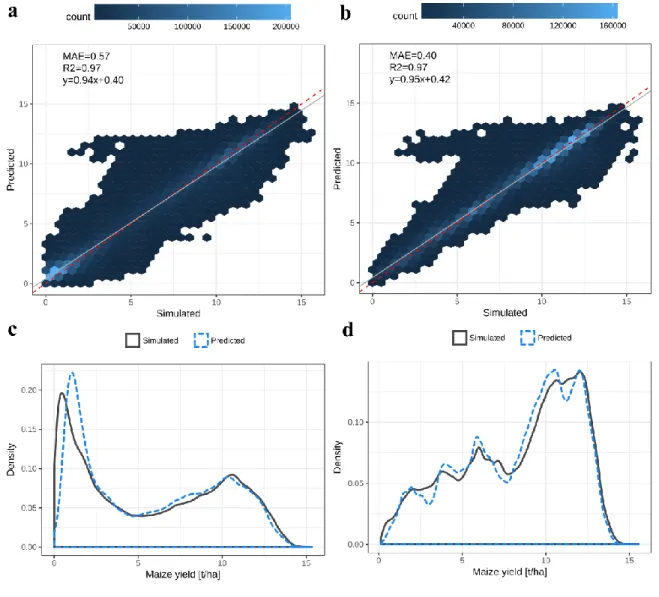
Table 2. Climate feature subsets used in the analyses. Besides indicated climate features (see 368
Table 1 for details), soil and site data, PHU, and LVP were considered in all training sets. 369
Feature subset Climate features considered Number of features
annual climate VARavYRcal, VARsumYRcal 23 growing season climate VARavGS, VARsumGS 23
monthly climate VAR_X (with X ≤ 6) 63
complete climate all features except VAR_X with x ≥ 7 151 370
2.5Performance metrics and model evaluation 371
2.5.1 Machine learning model performance compared to crop model simulations 372
Model performance was assessed using linear regression of (a) meta-model predictions 373
against the validation subset of global EPIC simulations and (b) downscaling predictions against 374
the high-resolution benchmark simulations for Mexico. Mean absolute error (MAE) was used as 375
a metric for mean model bias. Nash-Sutcliffe efficiency (NSE) was used as an indicator for the 376
accuracy of inter-annual yield variability. 377
The coefficient of determination R2 was calculated according to 378
21 𝑅2 = 1 −∑ (𝑌𝑟𝑒𝑓,𝑖−𝑌̂𝑝𝑟𝑒𝑑) 2 𝑛 𝑖=1 ∑𝑛𝑖=1(𝑌𝑟𝑒𝑓,𝑖−𝑌̅𝑟𝑒𝑓)2 (1) 379
where i is the number of the sample point (one simulation year-location) considered, n is 380
the total number of sample points across simulation units and years, Yref is the reference crop 381
yield, 𝑌̂𝑝𝑟𝑒𝑑 is the fitted yield, and 𝑌̅𝑟𝑒𝑓 is the arithmetic mean of reference samples. 382
MAE was calculated as 383 𝑀𝐴𝐸 =∑ |𝑌𝑝𝑟𝑒𝑑,𝑖−𝑌𝑟𝑒𝑓,𝑖| 𝑛 𝑖=1 𝑛 (2) 384
where Ypred,i is the machine learning model predicted value for data point i and Yref,i is the 385
corresponding EPIC simulated reference value. 386
NSE is a common metric for model performance over time, used especially in hydrology 387
(Nash and Sutcliffe, 1970). It is calculated using the same variables as the prior metrics but 388
separately for each simulation unit over time according to 389 𝑁𝑆𝐸 = 1 −∑ (𝑌𝑟𝑒𝑓,𝑡−𝑌𝑝𝑟𝑒𝑑,𝑡) 2 𝑚 𝑡=1 ∑𝑚𝑡=1(𝑌𝑟𝑒𝑓,𝑡−𝑌̅𝑟𝑒𝑓)2 (3) 390
where Ypred,t is the yield estimated by the meta model for year t and Yref,t the 391
corresponding reference. NSE can range from -∞ to +1 with NSE>0 indicating that model 392
predictions are more useful than the mean of reference data. As NSE is sensitive to both absolute 393
values and their temporal dynamics, it was in addition calculated for zero-centered yield values 394
(sample mean removed) in order to assess inter-annual yield variability alone, which is 395
considered a vital GGCM evaluation characteristic for climate (change) impact assessments (e.g. 396
Müller et al., 2017). 397
22
Evaluations were partly carried out at the level of major Koeppen-Geiger climate regions 398
(Figure S2) following the rules of Peel et al. (2007). Koeppen-Geiger regions were identified for 399
each 0.25° x 0.25° climate grid for the 31-year climatology of the AgMERRA dataset 1980-400
2010. 401
2.5.2 Model performance compared to regional statistics 402
The EPIC model itself and the global gridded EPIC-IIASA framework have been 403
evaluated and validated thoroughly at various scales from the agricultural plot (Kiniry et al., 404
1995; Gassmann et al., 2004; Izaurralde et al., 2006) to regional (Gaiser et al., 2010; Folberth et 405
al., 2012) and global assessments (Balkovič et al., 2014; Müller et al., 2017) finding good 406
agreement with reported yields. Here we provide a brief evaluation of model performance in 407
terms of inter-annual yield variability expressed as NSE (eq. (3)) for the top ten maize producing 408
municipios (second-level administrative units) of the major maize producing state Jalisco, where 409
crop management can be considered fairly stable and data quality reasonable. This also illustrates 410
an exemplary application of the machine learning framework. Reported maize yields were 411
obtained from SIAP (2018a). Crop yields are reported since the year 2003 at the second 412
administrative level, resulting in an evaluation period from 2003-2009 considering the time 413
period for crop model simulations (see Section 2.2). Besides the machine learning predictions 414
corresponding to the high-resolution input data for the crop simulations at the scale of Mexico 415
(see Section 2.3.1), predictions were also produced using monthly climate surfaces from 416
ClimateNA 5.60 (Wang et al., 2016) at a spatial resolution of 1 km x 1 km and a national soil 417
dataset (INEGI, 2004) besides HWSD to assess the impact of higher resolution climate data and 418
regional soil data products, a major application opportunity for the methodology presented 419
23
herein. Maize planting dates recorded in the year 2017 were obtained from SIAP (2018b). All 420
yields were de-trended linearly to correct for changes in management intensity. 421
2.6Computational framework 422
All computations, evaluations and plotting were done within the R software environment 423
(R Development Core Team, 2008). Machine learning models were built using the packages 424
specified in sections 2.4.1 and 2.4.2. Figures were produced using ggplot2 (Wickham, 2009). 425
Statistical analyses beyond linear regression were carried out with hydroGOF (Zambrano-426
Bigiarini, 2017). 427
3Results 428
3.1Global scale model performance for crop yields 429
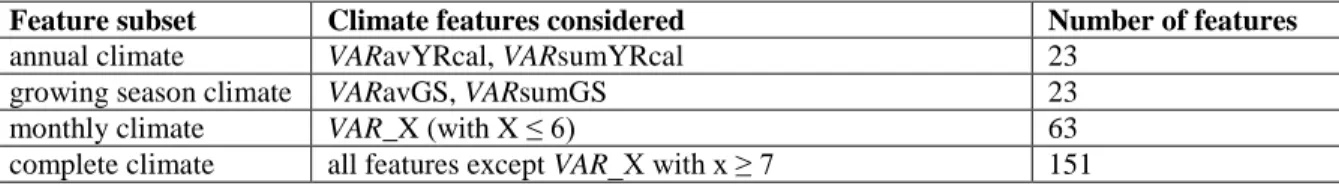
The global extreme gradient boosting meta-models for irrigated and rainfed maize yields 430
based on the full climate features show a near perfect fit and low mean bias in both cases (Figure 431
2a,b). Large over– and underestimations in predictions are rare. The first occur foremost at low 432
simulated yields, the latter at high ones with a negative trend beyond 12 t ha-1 (see Figure S3a,b 433
for residual plots). For rainfed yields, noticeable deviations in density distributions of EPIC 434
simulated and extreme gradient boosting predicted yields occur below 2 t ha-1 and around 6-7 t 435
ha-1 (Figure 2c). The density distributions are nearly identical for irrigated yields (Figure 2d).
24 437
Figure 2. Hexbin and regression plots for EPIC simulated and extreme gradient boosting 438
predicted crop yields in the validation dataset (25% of total samples) for (a) rainfed and 439
(b) irrigated conditions and corresponding density distributions for (c) rainfed and (d) 440
irrigated conditions. Red dashed and grey solid lines in (a) and (b) show 1:1 line and 441
regression, respectively. See section 3.4 and SI for random forest models. 442
25 3.2Performance of crop yield predictions for Mexico 443
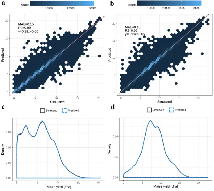
3.2.1 General performance and patterns 444
The accuracy of rainfed and irrigated yield predictions for Mexico at a high spatial 445
resolution (Figure 3a,b) is nearly up to that of the global validation data with 97% of variance of 446
EPIC simulated yields explained by the extreme gradient boosting models in both cases. Slopes 447
of the linear regressions are lower and the intercepts are higher than at the global scale indicating 448
biases at the lower and upper bounds of simulated yields. MAE increases by up to 0.5 t ha-1 but
449
is still considerably low concerning the mean of crop yield estimates. Overestimations by >100% 450
occur in both water management scenarios with a cluster of data points around 3.5 t ha-1 of EPIC 451
simulated yields. These are related to remaining nitrogen stress in few simulations (0.5% of 452
samples) due to extreme soil-climate combinations on which the automatic fertilizer application 453
of up to 500 kg N yr-1 does not suffice to fulfill plant requirements caused by vast losses of N in
454
runoff. Removing these simulations has no discernible effect on model performance (Figure S4). 455
The distributions of rainfed yield estimates and predictions exhibit a bimodal pattern with 456
over- and underestimation especially at the lower bound where the peak is shifted by about 1 t 457
ha-1 (Figure 3c). This is to a lesser extent also the case for the distributions of irrigated yield 458
estimates and predictions (Figure 3d). In addition, irrigated yields predicted by the extreme 459
gradient boosting model exhibit clustering, i.e. with overestimation peaks around 4, 5.5, and 10 t 460
ha-1 and valleys at 3 and 12 t ha-1, while EPIC simulated yields show a smoother distribution. 461
Using the more parsimonious climate feature sets decreases model performance (Table 462
S5) similar to the global scale validation data (Table S4). The largest decrease occurs for the 463
26
most set of growing season climate data, while again hardly any difference is found when using 464
the monthly climate features. 465
466
Figure 3. Same as Figure 2 but comparing the high-resolution downscaled predictions and 467
benchmark EPIC simulations for Mexico. 468
Comparing low-resolution simulations, high-resolution simulations, and high-resolution 469
machine learning predictions at the scale of a single state of Jalisco for rainfed maize yields in 470
27
the year 2000 shows that the machine learning predictions can fairly well reproduce the 471
heterogeneity seen in the high-resolution simulations (Figure 4a,c). Notable differences are 472
apparent in the region west of -104.5° and north of 20°, where the predictions are about 20% 473
lower than the simulation results and parts of the southern and northern state where predictions 474
are up to 40% higher (Figure 4d). Overall, the distributions of yields agree fairly well (Figure 475
4b), but the predictions omit moderate and very high yields, indicating peaks around 7.5 and 9 t 476
ha-1 and a valley at 10.5 t ha-1, which are not present in the simulations. Still, yield predictions
477
and simulations are correlated with R2=0.87 (Figure S5a). 478
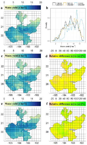
28 479
Figure 4. Examples of rainfed maize yields for the year 2000 in the state of Jalisco from (a) 480
high-resolution EPIC simulation, (c) high-resolution machine learning prediction, and (e) 481
global low-resolution simulation. (b) Shows the corresponding density distributions for 482
which yield estimates from the low-resolution simulations have been resampled to the 483
higher resolution to obtain at consistent sample sizes. (d) and (f) show the relative 484
differences of (c) and (e) compared to (a), respectively. Regressions and statistics are 485
presented in Figure S5a,b. The rectangular grid represents the 0.25° x 0.25° climate grid. 486
29
Expectedly, low-resolution EPIC estimates (Figure 4e) agree only with respect to large-487
scale patterns. Substantial overestimation by up to 60% occur in the central parts and 488
underestimation by up to 30% foremost in the west but also scattered at the subgrid level (Figure 489
4f). The yield distribution is biased towards higher yield estimates (Figure 4b) and the coefficient 490
of determination is R2=0.64 (Figure S5b). The arithmetic means at the state level are 9.06 t ha-1 491
for the high-resolution simulations, 8.85 t ha-1 for the predictions, and 10.15 t ha-1 for the low-492
resolution simulations, corresponding to an overestimation by 11.98% for the low-resolution 493
simulations and an underestimation by 2.31% for the extreme gradient boosting predictions. 494
Hence, despite remaining differences, the high-resolution predictions reproduce the 495
corresponding simulations quite robustly compared to the EPIC outputs derived from more 496
granular input data. 497
3.2.2 Reproduction of inter-annual crop yield variability 498
NSE is greater than zero in around 20-30% of all simulation units for predictions of 499
rainfed yields by the model based on calendar year climate features alone (Figure 5a-c). The 500
model trained with the full set of climate features in contrast shows a substantially better 501
performance, especially in tropic climates. If simulated and predicted yields are zero-centered 502
and only present cropland is considered, NSE performance turns out substantially better for both 503
feature sets (Figure 5d-f) and again to a very high degree for the extreme gradient boosting 504
model trained on the full climate feature set. 505
30 507
Figure 5. Violin plots of Nash-Sutcliffe Efficiency disaggregated by major Koeppen-Geiger 508
climate regions (see section 2.5) for the feature subsets using calendar year climate 509
variables only or all climate features. (a-c) All simulation units of Mexico with raw data 510
or (d-f) only simulation units with >5% maize harvest area and zero-centered yield 511
variability. Percentages indicate the fraction of simulation units with NSE>0. 512
Complementary statistics are provided in Table S6. The extent of the y-axis was limited 513
to -5 for better readability. 514
31
With sufficient irrigation water supply, NSE performance is overall lower while the 515
patterns remain quite similar, resulting in only few simulation units with NSE>0 for the model 516
based on annual climate data (Figure S6a-f). A key difference to rainfed yield estimates is the 517
lower performance in (semi-)arid regions, where inter-annual yield variability decreases 518
substantially if sufficient water is supplied. 519
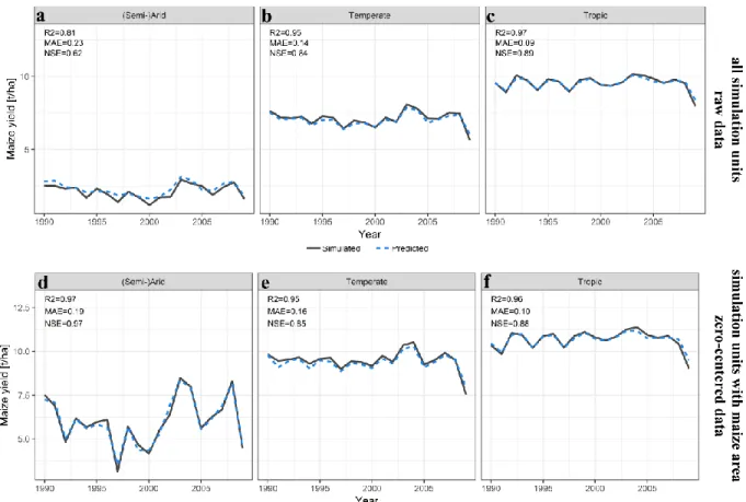
At a higher level of spatial aggregation – here the arithmetic mean for major Koeppen-520
Geiger climate regions –, inter-annual dynamics are well represented when considering all 521
simulation units (Figure 6a-c). Similar to the distributions presented above (Figure 5), 522
performance is best in tropic climates and poorest in (semi-)arid regions, but NSE is in all cases 523
well above zero and MAE < 0.25 t ha-1. If only present cropland is considered (Figure 6d-f), 524
performance decreases marginally in tropic and temperate climates, while it improves 525
substantially in (semi-)arid climate where mostly highly arid simulation units are now neglected 526
and predominantly simulation units with erratic rainfall remain (not shown). Foremost the latter 527
climate region shows that the yield predictions can quite well reflect both yield peaks and 528
valleys. 529
If sufficient irrigation water is supplied, the agreement with EPIC simulations in terms of 530
NSE decreases substantially in temperate climate if all simulation units are considered but 531
remains very similar in tropics and (semi-)arid climate (Figure S7a-c). For present cropland 532
alone, the agreement in terms of NSE decreases most in (semi-)arid climate compared to rainfed 533
yield estimates, followed by temperate regions. Predictions for the tropics still show very good 534
agreement. 535
32 536
Figure 6. Inter-annual dynamics of mean rainfed yields for each Koeppen-Geiger climate region 537
of Mexico (see section 2.5) considering (a-c) all simulation units or (d-f) only simulation 538
units intersecting with substantial maize harvest areas (see section 2.3.4). 539
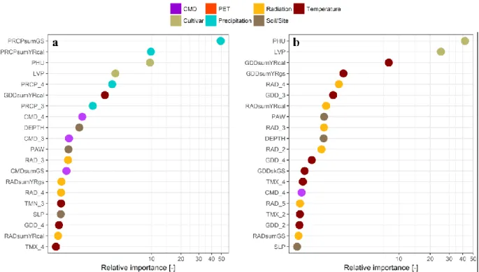
3.3Feature importance and the role of feature engineering 540
With rainfed water supply only, the sum of precipitation during the growing season 541
(PRCPsumGS) is the by far most important predictor (Figure 7a), followed by calendar year 542
precipitation PRCPsumYRcal, PHU, and LVP. Temperature, radiation, and soil-related features 543
are of moderate to minor importance. Soil variables matter only with respect to water 544
33
availability, driven by depth and PAW, which is a composite of texture, SOC, and depth. Other 545
soil variables, which are mostly related to nutrient availability, matter less due to the estimation 546
of yield potentials. With sufficient irrigation, the temporally static cultivar and management 547
characteristics PHU and LVP are the most important features, followed by the annual growing 548
degree day sum GDDsumYRcal and a wider set of transient climate features, which are 549
expectedly related to temperature and solar radiation (Figure 7b). Precipitation and ET-related 550
features do not occur among the top ranking features except for CMD_4. Among the soil 551
characteristics, again depth and PAW are the most relevant features. 552
Comparing the variable importance of different subsets of features for model training 553
(Figure S8; see Table 2 for feature subsets) shows that for rainfed water supply, precipitation- 554
and cultivar-related features are consistently the most important predictors (Figure S8a,c,e). 555
Beyond, the ranking of features depends on the feature set with PET derivatives exhibiting rather 556
low importance among climate features. Notably, soil characteristics beyond depth and PAW are 557
typically lowest ranking if occurring at all. With sufficient irrigation water supply, PHU and 558
LVP are consistently the most important features (Figure S8b,d,f) followed predominantly by 559
temperature and radiation indices. As for rainfed yield estimates, depth and PAW occur in all 560
feature set as moderately higher-ranking covariates. Precipitation- and PET-related features are 561
only present in the parsimonious models with 23 features in total, except for CMD_4 in the 562
model based on monthly features. 563
34 564
Figure 7. Feature importance for the extreme gradient boosting models for (a) rainfed and (b) 565
irrigated conditions. Only top 20 features (see Table 1 for details) are shown. The x-axis 566
is log(x+1) transformed for better readability. 567
3.4Random forests models compared to extreme gradient boosting 568
Statistical coefficients for the random forests predictions in the global validation dataset 569
are highly comparable to those from extreme gradient boosting (Table S4) with a marginal 570
tendency towards lower slopes and higher intercept and slope under rainfed conditions. 571
Predictions for Mexico in turn (Table S5) result typically in slightly higher intercepts and MAE 572
as well, but higher R2 especially for the parsimonious feature sets under irrigated conditions. 573
NSE statistics in contrast are almost consistently poorer. For the full set of climate 574
covariates under rainfed water management, the numbers of simulation units with NSE>0 are in 575
35
all cases lower or virtually equal (Table S8; c.f. Table S6). Most notable difference are apparent 576
for the models trained on the full climate feature set in tropic regions. This is even more 577
pronounced for irrigated conditions, where the number of simulation units with NSE<0 is up to 578
40% lower than the extreme gradient boosting predictions (Table S9; c.f. Table S7). 579
Accordingly, predictions aggregated to Koeppen-Geiger regions show also a poorer fit, 580
but differences are here less pronounced and apparent foremost in NSE statistics (Figure S12 and 581
Figure S13). This is most evident under rainfed conditions in (semi-)arid regions if all simulation 582
units are considered (Figure S12a-c). Under irrigated conditions, NSE is even negative in (semi-583
)arid climates, no matter whether all simulation units are considered or present cropland only, 584
(Figure S13a,d) and in temperate climate if all simulation units are considered (Figure S13b). 585
Variable importance remains structurally similar among feature subsets and water supply 586
regimes (Figure S14) compared to extreme gradient boosting (Figure 7; Figure S8) concerning 587
the overall ranking of features with some predictors moving up or down a few positions. A 588
striking differences, however, is that random forests rank also variables indicating distributions, 589
i.e. standard deviation, among the more important features, while extreme gradient boosting 590
predictions are foremost relying on sums and averages. 591
3.5Reproduction of reported inter-annual yield variability 592
The evaluation of inter-annual yield variability for the top producing municipios in 593
Jalisco (Figure S15) shows that NSE is positive in the majority of municipios and hence 594
satisfactory in all crop yield predictions from both EPIC and the extreme gradient boosting 595
models. Lowest median performance was found for the global simulations (EPIC global), 596
36
followed by the high-resolution EPIC simulations at the scale of Mexico (EPIC high-res) with a 597
slight tendency towards higher NSE. Interestingly, the median NSE for extreme gradient 598
boosting predictions (Predicted high-res) is higher than for the EPIC simulations at the same 599
resolution. This is mainly due to one municipio with rather poor performance in the simulations, 600
while the predictions (Predicted high-res) do not achieve very high performance in other 601
municipios where EPIC simulations result in up to NSE=0.8. The overall best rendition of inter-602
annual yield variability is produced by the machine learning predictions using 1k-resolution 603
monthly climate surfaces (Predictions 1k) and more so if a national soil data product is used 604
(Predictions 1k CRU x INEGI) with a median NSE of 0.42 as opposed to 0.20 in the high-605
resolution EPIC simulations (EPIC high-res). The CRU x HWSD combination in contrast results 606
in a lower median but higher maximum NSE. 607
4Discussion and Conclusions 608
4.1Model performance for downscaling of yield estimates 609
Performance of the meta-models for spatio-temporal downscaling of crop yield estimates 610
is exceptionally high in terms of linear regression statistics, and mean bias for both machine 611
learning methods (Table S4; Table S5). While the results are highly comparable among the two 612
methods, extreme gradient boosting shows moderately better results especially for inter-annual 613
yield variability (cf. Tables S6-9), which is of ample importance for climate impact studies (e.g. 614
Müller et al., 2017). In essence, substantial deviations of predictions from EPIC simulations 615
occur only for very low yields. Even here, this applies foremost to their absolute magnitude 616
while inter-annual yield variability is typically still very well reproduced although this is not an 617
37
implicit goal of the machine learning model optimization. In addition, the high skill in 618
reproducing irrigated yields stands out, as crop yield variability is known to be more strongly 619
dominated by variability in precipitation than temperature in most regions (e.g. Frieler et al., 620
2017). 621
Our results can hardly be compared to existing literature, as the spatio-temporal 622
downscaling of crop model outputs via meta-models has not yet been addressed to the authors’ 623
knowledge. Within the closely related, recently emerging field of crop model emulators, Blanc 624
and Sultan (2015) and Blanc (2017) developed polynomial models to predict yields for various 625
crops under climate change using unique parameterizations for the statistical models at the grid 626
cell level. Besides weather and soil data, they include CO2 as an additional dimension. These
627
structural differences (a) grid-cell level in the references vs scale-free approach here and (b) no 628
CO2 dimension in the present study render the comparison of results difficult. The authors of the
629
cited studies conclude that the statistical models provide reasonable results in the longer term. 630
However, the visual comparison of inter-annual yield variability for the Corn Belt during the 631
historic time period in Blanc and Sultan (2015) and the regional predictions presented in this 632
study suggest that the polynomial models may be suitable at the global scale and for longer term 633
assessments but not for regional impact studies. A similar statistical approach has been employed 634
by Oyebamiji et al. (2015) for a single GGCM finding that 62-93% of crop yield variability 635
produced by the GGCM can be explained by their multiple tier statistical model, which was as 636
well parameterized at the grid cell level. This indicates that so far no other methodologic 637
approaches can provide as accurate and flexible crop meta-models as the ones presented herein, 638
38
which are also virtually scale-free, free from a priori assumptions on relevant features, and truly 639
data-driven. 640
The very high accuracy of the machine learning models also allowed for detection of an 641
anomaly in the high-resolution EPIC simulations for Mexico, in which the automatic fertilizer 642
application failed due to extreme combinations of climate and soil (see Figure 3a,b and 643
associated text). This indicates that the method should also be tested for quality control of crop 644
model simulations. 645
4.2Feature engineering and feature importance 646
The evaluation of different feature subsets shows that even very basic features from 647
annual climate provide robust results when it comes to general regression metrics. This 648
highlights that these features should contain sufficient information for providing at least long-649
term mean crop yield and agricultural externalities surfaces. Monthly climate data are essential, 650
in contrast, to provide predictions of very high accuracy (Table S4, Table S5) and to capture 651
inter-annual crop-climate response accurately as reflected in the EPIC model (Figure 6). This can 652
be expected as crop growth processes are typically non-linear (Bonhomme, 2000) and crops’ 653
sensitivity to temperature and water supply can shift throughout the growing season. That is, for 654
instance, the case for drought stress susceptibility of maize yield formation, which is largest 655
during the second half of the growth cycle for maize (e.g. Gaiser et al., 2010) and is reflected in 656
the EPIC model within the calculation of an actual HI based on water stress (see section 2.1). 657
The feature importance of models for rainfed yield prediction is quite straightforward 658
with precipitation and other water-related features strongly dominating (Figure 7a). Static 659
39
variables PHU and LVP follow thereafter, rendering water availability the main driver for inter-660
annual yield variability, while especially PHU – a composite of growing season length and long-661
term temperatures – may rather serve as a proxy for the overall yield potential and thermal 662
growth conditions. If monthly climate statistics are considered, the third and fourth months have 663
the largest influence on rainfed yield predictions. This relates to the aforementioned non-linearity 664
of crop growth requirements and the crop’s higher sensitivity during the second half of the 665
growing season. 666
If sufficient water is supplied (Figure 7b), temperature- and solar radiation-related 667
features come to the fore. In the first case, these are not minimum or maximum temperatures 668
indices as such, but again growth effective temperature sums (here GDD). This corresponds 669
directly to the estimation of phenologic development in the EPIC model (see section 2.1), which 670
is driven by HU accumulation, while very high and very low temperatures cause stresses to the 671
crop, which is over large areas typically of minor importance compared to water deficits (e.g. 672
Schauberger et al., 2017). It is striking, however, that among the transient climate features, not 673
the growing season sum of GDD (GDDsumGS) is the most important feature, but annual GDD 674
(GDDsumYRcal). An explanation is that growing season features were calculated for the months 675
of the average length of vegetation period (feature LVP). Hence, GDDsumGS may in some years 676
exceed or fall below the actual PHU requirement, while GDDsumYRcal is a more robust annual 677
temperature index. 678
The low importance of soil covariates can be expected due to the simulation of yield 679
potentials. As shown in an earlier study (Folberth et al., 2016), the EPIC model itself is rather 680
insensitive to soil data if yield potentials are simulated, even more so with sufficient irrigation. 681
40
Hence, the only soil covariates of relevance here relate to water availability, i.e. soil depth and 682
PAW. Nutrient-related soil covariates in turn may even outweigh the importance of climate 683
features if no or little nutrients are supplied exogenously as nutrient supply can affect crop yields 684
by more than an order of magnitude (e.g. Folberth et al., 2013). Still, the spatial detail in Figure 685
4a,b shows that despite the low importance of soil and site covariates, yield patterns are very 686
well reproduced at the sub-climate grid (0.25° x 0.25°) level. This indicates that the soil and site 687
signal is sufficiently represented in the crop yield meta-model despite the comparably low 688
ranking of soil and site features (Figure 7). An increase in the importance of soil and site features 689
was found for the meta-model to predict crop available water (Supplementary Text S2), where 690
various hydrologically relevant covariates such as slope and soil hydrologic group rank higher 691
than for crop yield predictions or GSET (Figure S11). This emphasizes that approaches free from 692
assumptions on feature importance are required at least when moving away from crop yield 693
predictions towards agricultural externalities. 694
4.3Predictions of agricultural externalities 695
Agricultural externalities were assessed supplementary (Supplementary Text S2) to 696
evaluate the potential of machine learning algorithms to predict these as well, which is an 697
essential advantage of integrated crop growth models compared to purely statistical methods of 698
crop yield estimation. The very good results for GSET show that this is in principle feasible. The 699
slightly lower performance for CAW in turn indicates that there are limits under extreme 700
conditions: The very high values that are underestimated here (Figure S9c,d) occur in simulation 701
units with moderate to high precipitation, low slopes, and soils with high infiltration potential 702
(not shown). Capturing also such combinations may require an extension of the training data set 703
41
(see section 4.6). Overall, however, the results show that the computational framework used for 704
yield predictions can flexibly be transferred to other crop model outputs. Limitations can still be 705
expected for agro-environmental externalities that occur intermittently with daily peaks such as 706
emissions of certain greenhouse gases. 707
4.4Differences and advantages of employed machine learning approaches 708
Differences between the applied machine learning algorithms have been touched upon 709
above and are here summarized and complemented. In this study, random forests were found to 710
have lower performance in predictions with respect to inter-annual yield variability but showed 711
overall similar predictive accuracy, while also the importance of features for crop yield 712
predictions remained comparable (see section 3.4). From a practical point, however, the 713
computational cost of random forests is far higher than that of extreme gradient boosting. In the 714
case of the full climate feature set, it was here about nine hours versus one on the same 32 core 715
cluster (Figure S16). Even if the number of trees was reduced, which may not cause substantial 716
trade-offs in accuracy (Figure S1), the time requirement can be assumed at least four times 717
higher. While common gradient boosting methods may show low computational performance 718
due to sequential tree building, the extreme gradient boosting approach has markedly high 719
efficiency due to parallelization as already evaluated in its original publication (Chen and 720
Guestrin, 2016). 721
Although the quantification of prediction uncertainty is beyond the scope of this study, it 722
is worth mentioning that for random forests there are established methods to quantify prediction 723
intervals and hence uncertainties associated with predictions (e.g. Meinshausen, 2006) for which 724