Middlesex University Research Repository
An open access repository of
Middlesex University research
http://eprints.mdx.ac.ukLiu, Yilin (2008) Bayesian modelling of the spatial distribution of road
accidents. PhD thesis, Middlesex University.
Available from Middlesex University’s Research Repository at
http://eprints.mdx.ac.uk/13419/
Copyright:
Middlesex University Research Repository makes the University’s research available electronically.
Copyright and moral rights to this thesis/research project are retained by the author and/or other copyright owners. The work is supplied on the understanding that any use for
commercial gain is strictly forbidden. A copy may be downloaded for personal,
non-commercial, research or study without prior permission and without charge. Any use of the thesis/research project for private study or research must be properly acknowledged with reference to the work’s full bibliographic details.
This thesis/research project may not be reproduced in any format or medium, or extensive quotations taken from it, or its content changed in any way, without first obtaining permission in writing from the copyright holder(s).
If you believe that any material held in the repository infringes copyright law, please contact the Repository Team at Middlesex University via the following email address:
Middlesex University Research Repository:
an open access repository of
Middlesex University research
http://eprints.mdx.ac.uk
Liu, Yilin, 2008.
Bayesian modelling of the spatial distribution of road accidents. Available from Middlesex University’s Research Repository.
Copyright:
Middlesex University Research Repository makes the University’s research available electronically. Copyright and moral rights to this thesis/research project are retained by the author and/or other copyright owners. The work is supplied on the understanding that any use for commercial gain is strictly forbidden. A copy may be downloaded for personal, non-commercial, research or study without prior permission and without charge. Any use of the thesis/research project for private study or research must be properly acknowledged with reference to the work’s full bibliographic details. This thesis/research project may not be reproduced in any format or medium, or extensive quotations taken from it, or its content changed in any way, without first obtaining permission in writing from the copyright holder(s).
If you believe that any material held in the repository infringes copyright law, please contact the Repository Team at Middlesex University via the following email address:
Bayesian Modelling of the Spatial
Distribution of Road Accidents
Yilin Liu
A thesis submitted to Middlesex University in partial fulfilment of the
requirements for the degree of Doctor of Philosophy
Middlesex University Business School
April 2008
PAGE
NUMBERING
AS ORIGINAL
Acknowledgements
This thesis is the result of four and half years of work whereby many peo-ple have assisted and supported in various forms. I would like to have this opportunity to express my gratitude for all of them. I am extremely grateful to Middlesex University for financially supporting the completion of PhD as well as the presentations of my papers in two conferences and to the Research Office in Business School for providing necessary supports during my study.
My first supervisor, David Jarrett, deserves a special mention. He made ex-cellent supervision on the progress of my work and always was available when I needed his advice. He provided many valuable comments on earlier versions of the thesis. He is the one who brought my interests in the areas of road safety and applied statistics. I have learned a lot from him. To my second supervisor Chris Wright, thank you for your support and guidance, and giving thoughtful comments on the draft of thesis. Chris introduced the area of road safety to me and always encouraged me during my study. He also helped me obtain the right to use some data needed for this study from external organisations. To Jeff Evans, thank you for your advice and encoUf-agement during my study. I would also like to thank late Ken Lupton for introducing the Ordnance Survey data and geographical information systems tome.
This study involved the analysis of a large amount of data. I would like to thank Jacqui Bates and Sonal Ahuja of Matt MacDonald Ltd, Anne Patrick of the Ordnance Survey, and Solihull MBC and Coventry City Council for providing access to the SPECTRUM database. The accident data, STATS 19, were distributed by UK Data Archive (Crown Copyright) and authored by Department for Transport.
Abstract
This research aims to develop Hierarchical Bayesian models for road accident counts that take account of the spatial dependency in the neighbouring areas or sites. The Poisson log-linear model is extended by introducing a second level of random variation that includes a conditional autoregressive (CAR) component. Both models for accidents at the area level and models for acci-dents on a road network are developed. Areal models are fitted using data for counties and districts in England covering two different periods and data for wards in the West Midlands region in 200l. Network models are fitted to link data for the MI motorway and to junction data for the city of Coventry.
Results show that, in most cases, adding a spatial (CAR) component to con-ventional models produces better estimates of the expected number of acci-dents in an area or at a site. Signs of the coefficients for explanatory variables, including level of traffic and road characteristics, are consistent with expecta-tion. Levels of the spatial effects in a CAR model reflect the relative influence of the unknown or unmeasurable explanatory variables on the expected num-ber of accidents. Results from models at the local authority level in the 2000s show that spatial effects are positive in London boroughs and are negative in most metropolitan districts. For accidents at the ward level in the West Mid-lands, the performance of the CAR model is similar to that of the non-CAR model which includes log-normal random effects and metropolitan county ef-fects. For models of accidents on the MI, several links are identified to have positive and fairly large spatial effects. For Coventry junction accidents, the CAR model does not perform better than the non-CAR model. Approaches to including temporal effects in spatial models when data cover two or more periods and jointly modelling different types of accidents are also proposed and examined.
Two applications of the CAR models developed in this research are intro-duced. The first application is about predicting the number of accidents in a local authority in a new year based on previous years' data. One advantage of using the CAR model is that it produces more precise predictions than the non-CAR model. The second application of the CAR model is a new ap-proach for site ranking. The sites selected by such a criterion are those with high risks caused by some unknown or unmeasured factors (for instance, cur-vature or gradient of roads) which are spatially correlated. Further on-site investigation will be needed to identify such factors.
Contents
1 Introduction 1.1 Background
1.2 Aims of the research 1.3 Overview of the thesis
2 Statistical models for road accident data
2.1 The role of statistical models in road safety research. 2.2 General description of the STATS19 data.
2.3 Statistical models for accident frequencies 2.3.1 Poisson model . . . . 2.3.2 Negative binomial (NB) model. 2.3.3 Empirical Bayes methods
2.4 Limitations of conventional models. 2.5 Spatial analysis of road accidents . .
2.5.1 2.5.2
Spatial cluster identification Models with spatial aspects 2.6 Bayesian methods for data analysis .
2.6.1 Applying Bayes' Theorem 2.6.2 Bayesian computation . .
2.6.3 Estimation of parameters and model comparison 2.7 Bayesian models for numbers of road accidents . . . . .
\' 1 1 6 8 12 13 14 16 17 19 21 23 27 28 29 32 32 33 35 38
3 Bayesian models for spatial data 3.1 Bayesian spatial models. . .
3.1.1 General introduction of spatial data analysis . 3.1.2 Conditional autoregressive (CAR) model 3.1.3 Spatial moving average models
3.2 Extensions of univariate CAR models 3.2.1 Multivariate CAR models .. 3.2.2 Models with spatio-temporal effects 3.3 Moran's I statistic .
3.4 Edge effects . . . .
4 Methodology: Spatial models for accident frequencies 4.1 Univariate models . . . .
4.1.1 Poisson log-linear model
CONTENTS
4.1.2 Poisson regression model with log-normal random effects 4.2 Univariate spatial models . . . .
4.2.1 Poisson regression model with regional (fixed) effects 4.2.2 Poisson regression model with spatial random effects 4.2.3 Spatial neighbours list and weighting choice.
4.2.3.1 Neighbours list. . 4.2.3.2 Weighting choice 4.3 Univariate models with temporal effects 4.4 Poisson model with spatio-temporal effects 4.5 Multivariate models . . . .
4.6 Model fitting and checking
4.7 Posterior distribution of Moran's I
5 Methodology: Variables and data
5.1 Accident data and response variables .
5.2 Choice and measurement of explanatory variables
-w
41 41 43 47 48 48 50 52 53 55 56 56 57 57 57 5860
60
6567
67
69
71 73 75 7576
CONTENTS 5.2.1
5.2.2 5.2.3
Traffic and road characteristics. Proxy variables for traffic . . .
Characteristics of the geographical area 5.3 Data collection and preparation . . . .
5.3.1 Data for local authorities in England from 1983 to 1986 5.3.2
5.3.3 5.3.4 5.3.5
Data for local authorities in England from 2001 to 2005 Data for wards in the West Midlands in 2001
Data for the MI. . . . Data for junctions in Coventry
77 79 79 79 80 82 84 86 89
6 Areal models for accident frequencies 91
6.1 General description . . . " 91 6.2 Models for accidents at the local authority level in England from 1983 to
1986 . . . 93 6.2.1 Models for accidents in a single year.
6.2.2 Models for four years' data . . . .
94 99
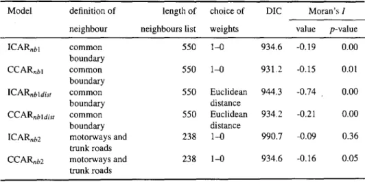
6.2.2.1 DIC and spatial correlation 99
6.2.2.2 Estimated parameters of the explanatory variables 107 6.2.2.3 Temporal correlation . . . 112 6.3 Models for accidents at the local authority level in England from 2001 to
2005 6.3.1 6.3.2 6.3.3 6.3.4 . . .
Description of the models DIC and spatial correlation . Maps of spatial effects
Temporal correlation . 115 116 118 120 125 6.3.5 Estimated coefficients 126
6.4 Models for accidents at the ward level in the West Midlands in 2001 132 6.4.1 Relationships of the variables
6.4.2 Description of the models .,
6.4.3 Models comparison and interpretation
132 132 134
6.4.4 Estimated coefficients .. 6.4.5 More on the spatial effects 6.5 More on residual spatial autocorrelation 6.6 Conclusion . . . . . . .
7 Models of accidents on a road network 7.1 Models for accidents on MI. . .
7.1.1 Some descriptive statistics 7.1.2 Fit of the models . . . . . 7.1.3 Estimates of the parameters
7.1.4 More on residual spatial autocorrelation 7.2 Junction accidents in Coventry
7.3 Conclusion .. . . . .
8 Applications of the models
9
A
8.1 Prediction of accident counts 8.2 Ranking the sites ..
8.2.1 Background.
8.2.2 Model-based ranking 8.2.3 More on the Mllinks .
Conclusion
9.1 Summary of the thesis 9.2 Findings from the analyses 9.3 Limitations of the research
9.4 Main contributions of the research 9.5 Suggestions for further research
Lists of local authorities and wards
B Parameter estimates for selected areal models (1983 - 1986)
CONTENTS 135 139 140 142 145 145 145 148 150 151 157 159 160 160 167 167 169 175 177 177 179 184 187 188 192 205
C Parameter estimates for selected areal models (2001 - 2005) D Parameter estimates for selected ward models (West Midlands) E Predictions using the non-CAR model
F WinBUGS codes for selected models F.1 Areal models (1983 - 1986) . F.2 Areal models (2001 - 2005) . F.3 Ward models (West Midlands) FA Link models for the MI. . . . F.5 Junction models for Coventry . F.6 Areal model for prediction
References CONTENTS 211 217 220 224 224 226 231 234 235 236 250 IX
List of Figures
2.1 Rectangular grids for areal models .. 2.2 Spatial dependency among the grids. 2.3 A node graph for junctions. . . . 2.4 Spatial dependency among the nodes. 2.5 A linear network. . . . .
4.1 Incomplete map of London boroughs . 4.2 Accidents on a road network.
4.3 A node-link-cell system. ..
4.4 Map of part of Southern England in 1980's.
5.1 Layout of the motorways in England .. 5.2 Node-link graph for the Ml. . . .
5.3 Neighbours structure of major junctions in Coventry.
6.1 Relationships between the variables in logarithmic forms for accidents in 1986: 'Fatal' for fatal accidents; 'Serious' for serious accidents; 'Slight' for slight accidents; 'Traffic' for traffic volume in million vehicle-km; 'Road' for road length in km; 'Vehicle' for number of registered vehicles
24 25 25 26 31 61 63 64 66 86 88 90 in thousand. . . ., 94
LIST OF FIGURES 6.2 Maps (England) of standardized residuals for serious accidents: (a) model
PLNre (Poisson model with log-normal random effects and metropolitan effects); (b) model CCARnbl (convolution CAR model whose neighbours list is determined by the boundaries); (c) model CCARnb2 (convolution CAR model whose neighbours list depends on the layout of the road
net-work). . . .. 98 6.3 Maps (London boroughs) of standardized residuals for serious accidents
- using the same models as in Figure 6.2. . . . 98 6.4 Residual maps for model PL (Poisson log-linear model): fatal accidents. 104 6.5 Residual maps for model PLNre (Poisson model with log-normal random
effects and metropolitan county effects): fatal accidents. 105 6.6 Residual maps of London boroughs for model PL: fatal accidents. 105 6.7 Residual maps of London boroughs for model PLNre: fatal accidents. 106 6.8 Residual maps for model PLNre (Poisson model with log-normal random
effects and metropolitan county effects): serious accidents. . . .. 106 6.9 Residual maps of London boroughs for model PLNre: serious accidents. 107 6.10 Residual maps for model CCAR(t)nb3roadtemp2 (convolution CAR model
with temporal effects, modelled by a first order autoregressive prior and its neighbours list depends on the layout of the road network): senous accidents. . . . . . 108 6.11 Residual maps of London boroughs for model CCAR(t)nb3roadtemp2:
se-rious accidents. . . 109 6.12 95% credible intervals of the coefficients for the explanatory variables in
model PLNre&temp2 for fatal accidents . . . 110 6.13 95% credible intervals of the coefficients for dummy variables in model
PLNre&temp2 for fatal accidents: 'Lon' for London boroughs; 'Man' for Great Manchester; 'Mer' for Merseyside; 'SYork' for South Yorkshire': 'T&W' for Tyne and Wear; 'WMid' for \Vest Midlands: '\VYork' for
West Yorkshire. . . 110
LIST OF FIGURES 6.14 95% credible intervals of the coefficients for the explanatory variables in
model PLN: serious accidents. . . . . 111 6.15 95% credible intervals of the coefficients for the explanatory variables in
model CCAR(t)nb3roadtemp2: serious accidents. . . III
6.16 95% credible intervals of the coefficients for the dummy variables in model PLNre: serious accidents (for full names of metropolitan counties,
see Figure 6.13). . . . 112 6.17 95% credible intervals of the coefficients for the explanatory variables in
model PLN: slight accidents. . . 112 6.18 95% credible intervals of the coefficients for the explanatory variables in
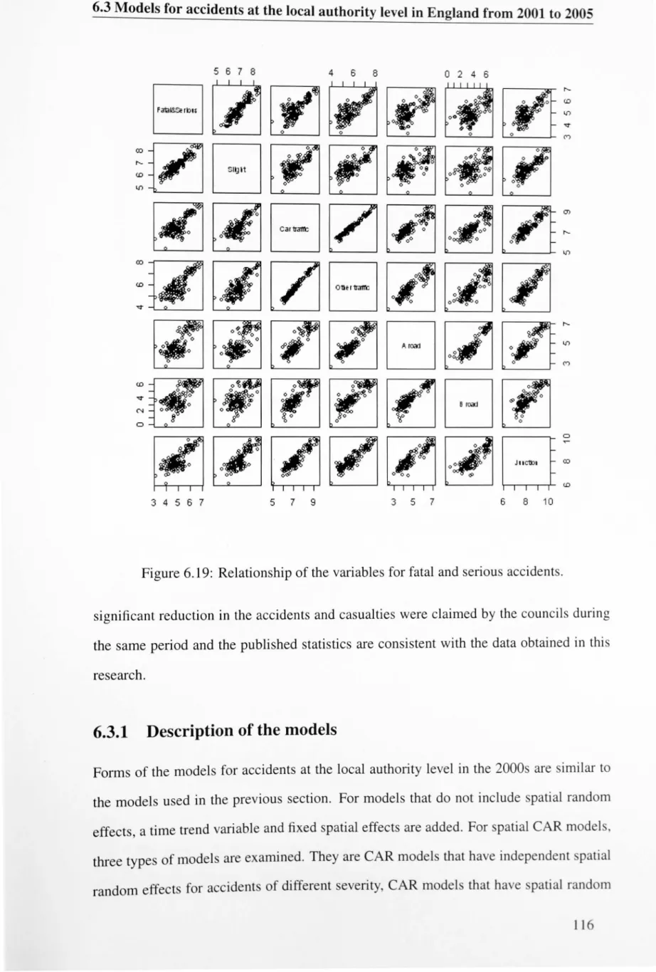
model CCAR(t)nb3roadtemp2: slight accidents. . . . 113 6.19 Relationship of the variables for fatal and serious accidents. . 116 6.20 Trend in the fatal and serious accidents: 2001-2005. 117
6.21 Trend in the slight accidents: 2001-2005. 117
6.22 Trend in the fatal and serious accidents for selected local authorities: 1. Lambeth~ 2. Devon~ 3. Lincolnshire~ 4. Oxfordshire~ 5. Hertfordshire; 6.
Hampshire; 7. Kent . . . 118 6.23 95% credible intervals of the spatial effects in model CCAR(t)tr.temp
in 2001: 'wm' for West Midlands; 'lon' for London boroughs; 'sy' for South Yorkshire; 'wy' for West Yorkshire; 'mer' for Merseyside; 'man'
for Great Manchester; 'ty' for Tyne and Wear . . . 122 6.24 England maps of the spatial effects for model CCAR(t)tr.temp: fatal and
serious accidents. . . 123 6.25 England maps of the spatial effects for model CCAR(t)tr.temp: slight
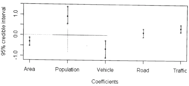
ac-cidents. . . . 12.+ 6.26 Credible intervals of the coefficients in model PLNtr for fatal and serious
accidents: explanatory variables from the left to the right are area, popu-lation, length of A-roads, length of B-roads, length of minor roads, traffic by other vehicles, traffic by cars and number of nodes. 128
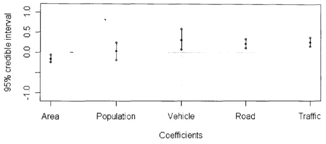
LIST OF FIGURES 6.27 Credible intervals of the coefficients in model CCAR(t)tr.temp for fatal
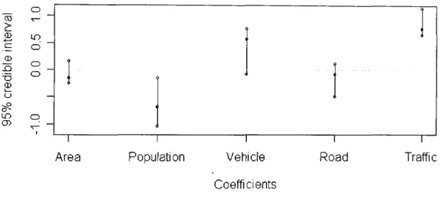
and serious accidents: same explanatory variables as in Figure 6.26. . . . 129 6.28 Credible intervals of the coefficients in model PLNtr for slight accidents:
same explanatory variables as in Figure 6.26. . . . 130 6.29 Credible intervals of the coefficients in model CCAR(t)tr.temp for slight
accidents: same explanatory variables as in Figure 6.26. . . 131 6.30 Relationships of selected variables in logarithmic form: 'FS' for the fatal
and serious accidents; 'SL' for the slight accidents; 'Major' for the length of major roads; 'Minor' for the length of minor roads; 'Junction' for the n.umber of junctions; 'Travell' to 'TraveI4' for population travelling to
work by car as driver, by car as passenger, on foot and by bus respectively. 133 6.31 Credible intervals for the coefficients of the explanatory variables in model
PLN for fatal and serious accidents: explanatory variables are in turn pop-ulation, area, length of major, length of minor, number of nodes, popula-tion travelling to work by bus, by car as driver, by car as passenger and on foot respectively. . . 137 6.32 Credible intervals for the coefficients of the explanatory variables in model
MVCCAR for fatal and serious accidents: same explanatory variables as
in Figure 6.31. . . . 137 6.33 Credible intervals for the coefficients of the explanatory variables in model
PLN for slight accidents: same explanatory variables as in Figure 6.31. . . 138 6.34 Credible intervals for the coefficients of the explanatory variables in model
MVCCAR for slight accidents: same explanatory variables as in
Fig-ure 6.31. . . 138 6.35 Map of the posterior medians of the spatially structured random effects in
model MVCCAR: fatal and serious accidents. . . 139 6.36 Map of the posterior medians of the spatially structured random effects in
model MVCCAR: slight accidents. . . 140
LIST OF FIGURES 6.37 Values of Moran's I in Bayesian residuals from model PLtr: (a) based on
true y; (b) based on predicted values for y . . . 141 6.38 Values of Moran's I in Bayesian residuals from model PLNtr: (a) based
on true y; (b) based on predicted values for y. . . . . 142 6.39 Values of Moran's I in Bayesian residuals from model CCAR(t)tr.temp:
(a) based on true y; (b) based on predicted values for y. . . . . 143
7.1 7.2
Box plots for the accident data from 1999 to 2005.
Spatial correlograms for the accident count per kilometre on the MI. 7.3 Spatial correlograms for the accident count per vehicle-kilometre on the
MI . . . . 7.4 Spatial correlograms for the AADF on the MI. 7.5 Relationship between variables . . . .
146 147
147 148 149 7.6 Val ues of Moran's I in Bayesian residuals from model PLN. 152 7.7 95% credible intervals of log-normal random effects (v) from model PLN. 153 7.8 Values of Moran's I in Bayesian residuals from model PL: (a) based on
true y; (b) based on predicted values for y . . . 154 7.9 Values of Moran's I in Bayesian residuals from the intrinsic CAR model:
(a) based on true y; (b) based on predicted values for y. . . . . 155 7.10 95 % credible intervals of spatially structured random effects (8) from the
intrinsic CAR model. . . 156 7.11 95% credible intervals of spatially structured random effects (8) from
model CCARtr. . . 156 7.12 95% credible intervals of unstructured random effects (v) from model
CCARtr . . . . 7.13 Accident counts by junction types
8.1 Comparisons of prediction results from the non-CAR model and the CAR model by using the posterior median of
A.
8.2 Predictions for London boroughs. . . . .
157 158
163
16-1-LIST OF FIGURES 8.3 Predictions for metropolitan districts ..
8.4 Predictions for unitary authorities. . . 8.5 Predictions for other local authorities.
8.6 Trend of fatal and serious accidents in unitary authorities where y is
sig-8.7 8.8 8.9 8.l0 8.11 8.12 9.1 E.l E.2 E.3 E.4
nificantly under-estimated: l. Bracknell Forest; 2. Darlington; 3. Redcar and Cleveland; 4. Blackpool; 5. Milton Keynes; 6. York; 7. Brighton and Hove. I • • • • • I • • • • • • • • •
Comparisons of ranking results: A .. Comparisons of ranking results: B .. Posterior ranks by the accident rates. Spatial random effects for the M 1 links.
Posterior ranks by the spatial random effects for the Ml links. Posterior ranks by the spatial random effects in local authorities.
Accidents on a road network. . . .
. . .
Predictions for London boroughs. Predictions for metropolitan districts .. Predictions for unitary authorities.
..
Predictions for other local authorities.165 166 167 168 170 171 172 172 173 174 189 220 221 222 223 X \'
List of Tables
6.1 Summary of the model fits for fatal accidents in 1986 . . . .. 95 6.2 Summary of the model fits for serious accidents in 1986, excluding CAR
models. . . .. 96 6.3 Summary of the model fits for CAR models for serious accidents in 1986 96 6.4 Summary of the model fits for fatal accidents (1983-1986) . 100 6.5 Summary of the model fits for serious accidents (1983-1986) 100 6.6 Summary of the model fits for slight accidents (1983-1986) . 102 6.7 Summary of the variance parameters in selected CAR models . 103 6.8 Temporal correlation coefficients for residuals from model PLNre for fatal
accidents 113
6.9 Temporal correlation coefficients for residuals from model CCAR(t)nb3road
for serious accidents 114
6.10 Temporal correlation coefficients for residuals from model CCAR(t)nb3road
for slight accidents . . . 114 6.11 Temporal correlation coefficients in residuals for serious accidents from
model CCAR(t)nb3roadtemp2 . . . 114 6.12 Temporal correlation coefficients in residuals for slight accidents from
model CCAR(t)nb3roadtemp2 . . . 114 6.13 Summary of the multivariate models for accidents in England in the 2000s 118 6.14 Summary of the variance parameter
re
for the spatial component in aLIST OF TABLES 6.15 Temporal correlation coefficients for residuals from model CCAR(t)tr for
fatal and serious accidents . . . 126 6.16 Temporal correlation coefficients for residuals from model CCAR(t)tr for
r
h 'ds 19 t aCCl ents . . . 126 6.17 Temporal correlation coefficients for residuals from model CCAR(t)tr.temp
for fatal and serious accidents. . . 126 6.18 Temporal correlation coefficients for residuals from model CCAR(t)tr.temp
for slight accidents . . . . . . . 6.19 Summary of the model fits for accidents in the West Midlands
126 134
7.1 Summary of the model fits for accidents on the Ml from 1999 to 2005 149
A.1 Lists of local authorities in Englands in the 1980s A.2 Lists of local authorities in Englands in the 2000s A.3 Lists of wards in the West Midlands . . .
B.1 Parameter estimates for fatal accidents B.2 Parameter estimates for serious accidents B.3 Parameter estimates for slight accidents
C.1 Model PLtr C.2 Model PLtr-fe C.3 Model PLtr-re
CA
Model PLNtrC.5 Model CCAR(t)tr.temp
C.6 Model MVCCAR( t)tr. temp.mv
D.1 Model PLN D.2 Model PLNre D.3 Model MVCCAR.mv 192 196 200 205 207 209 211 212 213 214 215 216 217 218 219 .. X\,ll
Chapter 1
Introduction
1.1 Background
Every year in the world, road accidents cause injury and death, and result in a serious economic burden. Although in Great Britain the numbers of people killed and seriously injured have been reducing year by year, road safety still remains a serious problem. There were 280,840 casualties and 200,700 reported road accidents involving personal injury in Great Britain in 2005 (Department for Transport, 2006c). The total cost-benefit value of prevention of road accidents in 2005 was estimated to be over £18 billion (Department for Transport, 2007 a).
Against this background, in March 2000 a new road safety strategy 'Tomorrow's Roads-Safer for Everyone' was published by the government (see Department for Trans-port, 2001). It establishes challenging casualty reduction targets to be achieved by 2010. Compared with the baseline averages for 1994 to 1998, it aims to achieve:
1. a 40% reduction in the number of people killed or seriously injured in road acci-dents;
2. a 50% reduction in the number of children killed or seriously injured;
3. a 10% reduction in the slight casualty rate.
While good progress has been made towards the government targets, further reductions in casualties are needed. Numbers of casualties are closely related to the numbers of road
1.1 Background accidents that involve injuries. Therefore, any reduction in casualties is associated with a reduction in injury accidents. In order to reduce annual road accidents at the national level, similar targets for reductions in accidents are set at the regional level, for instance for local authorities. In addition, to improve road safety, causes of road accidents and the relationship between numbers of accidents and relevant factors, such as the level of traffic and road geometry, need to be investigated and studied.
As described by Ogden (1996), road traffic may be considered as a system that consists of various components. These components, such as the human, the vehicle and the roads, interact with each other. An accident may be considered as a failure in the system. The UK Department of Transport (Department of Transport, 1986) defines an accident as 'a rare, random and multi-factor event always preceded by a situation in which one or more persons have failed to cope with their environment'. Whether motivated by a humanitar-ian, public health or economic concern, the analysis of previous accident data is needed in road safety research. Statistical methods have been used in this area for a long time. With the development of the theory of generalized linear models (McCullagh and NeIder, 1989), improved methodologies for analysing road accidents become available. However, researchers face more challenges today. The number of journeys and the volume of traffic on the road become greater and greater especially in the developing countries. The road network structure becomes more complicated. There are more interactions between road users and the road environment. All these situations generate more information and more complex road user behaviour for researchers to cope with.
The approach to modelling of numbers of road accidents has experienced several stages in the development of statistical technique. Many statistical models have been developed to relate the accident count to demographic characteristics, road geometry and traffic characteristics (see, for instance, Jarrett et aI., 1989; Miaou, 1994; Milton and Man-nering, 1998). The response variable is usually an accident frequency, that is, the total number of accidents of a particular type (for instance, determined by severity) in a wider geographical area (for instance, a local authority) or at a site (for instance, a link or a junction) during a fixed period of time. It is usually assumed to be Poisson distributed.
1.1 Background However, the mean of the Poisson distribution can vary from area to area or from site to site and depends on the characteristics of the area or site, such as the level of traffic and road geometry. In order to relate the accident count to such explanatory variables, con-ventional approaches usually apply generalized linear models, fitted by maximum like-lihood. Maher and Summersgill (1996) give a broad review of the statistical methodol-ogy for accident models. The Poisson log-linear model and the negative binomial model are two well-known forms of model in road safety research. They are special instances of generalized linear models. The former does not perform well when the data display
over-dispersion, that is the residual variance is larger than the fitted Poisson mean. Such
over-dispersion can be taken account of by introducing an extra level of random effects that follow a gamma distribution in the Poisson mean. This leads to a negative binomial model that is much used in recent road safety research.
Models of accidents at different spatial levels should be used for different research purposes. In this thesis, models of accidents at the local authority or ward level are called
areal models and models of accidents at sites in a road network are called network models.
Areal models can be used to study the relationship between accident frequencies and factors like road conditions and economic development. They can also be used to compare accident frequencies in different administrative areas, such as local authorities, during the same period or to study changes in accident frequencies in an area in different years. See for instance Jarrett et al. (1989)~ Levine et al. (1995b)~ Miaou et al. (2003). Network models look at road accident frequencies at a more local level (on links or at junctions) and are usually developed to investigate the relationship between accident frequencies and contributory factors such as traffic flow and features of road geometry like road width, number oflanes and type of junction (see, for instance, Layfield et aI., 1996~ Summersgill et aI., 1996, 2001 ~ Walmsley, Summersgill and Payne, 1998). They can also be used for prediction (see, for instance, Greibe, 2003~ Mountain et aI., 1996; Qin et aI., 2003). Moreover, they can be applied to identify high-risk sites and to evaluate the effectiveness of engineering treatments on selected sites (see, for instance, Hauer, 1997; Miaou and Song, 2005; Mountain et aI., 1995a).
1.1 Background The performance of areal models and network models with respect to the above men-tioned research purposes depends on how precisely the expected accident frequency in an area or at a site can be estimated, which in tum is determined by the explanatory power of the statistical models. In principle, if all the contributory variables for road accidents could be identified and measured, and if the correct form of the model were known, the expected accident frequency would be estimated well. However, in practice, variables like traffic levels cannot be measured precisely and there are other contributory factors that are difficult to measure or even not known. In addition, a 'true' model for accident counts is not known. Therefore, a great challenge in road safety research is to improve statistical models for road accidents by taking account of contributory factors that are not directly measured by the explanatory variables. Under such circumstances, there are several ways to think about the problem.
First, if data for some contributory factors are not available, is it possible to find vari-ables that can be measured and used as proxies for the contributory factors? Sometimes, the answer will be yes. For instance, Bailey and Hewson (2004) and Noland and Quddus (2004) use employment and resident population as proxies for traffic levels. However, proxy variables cannot be found for all the contributory factors. Moreover, one limitation of using the proxies is that they are not best approximations to true explanatory variables and so will introduce measurement error bias (see Maher and Summersgill, 1996).
Another way to account for the unobserved or unmeasurable contributory factors is to consider the information that accident data contain. Accidents can be categorised by features like severity or road class. When multiple response models are developed for different types of accidents (for instance, determined by severity), it is possible that there are some common contributory factors for different types of accidents. When such factors are not included in the model, the correlation in the multiple response variables will not be fully explained by the model. But since the common contributory factors may have similar influence on the expected numbers of accidents of different types, the variation in the response variables due to such factors could be partly explained by introducing some random effects in the Poisson means that model the correlation in the expected numbers
1.1 Background of accidents of different types. Studies that jointly model different types of accidents include Tunaru (2002) and Song et al. (2006), both of which use a Bayesian modelling approach.
A further way of thinking about the effects of the unobserved or unmeasurable contrib-utory factors is to consider the characteristics of accident models. Both areal models and network models of road accidents are a type of spatial model because the observational unit is a location. Spatial data are collected and aggregated over space and likely to be spatially correlated. For areal models, factors like the extent of development and urban-ization are more likely to be similar in neighbouring areas. For network models, factors such as traffic levels and road geometry (for instance, curvature and gradient) are likely to be spatially correlated for neighbouring sites. When such factors are not measured perfectly or are unmeasurable, variation in the response variables cannot be completely explained. However, since such factors are often spatially correlated, by introducing some appropriate form of spatial random effects in the models, variation in the response vari-ables due to these factors can be partly explained (see Besag, in his contribution to the discussion of McCullagh, 2002). Therefore, better estimates of the expected numbers of accidents in different locations can be achieved.
The spatial correlation in the contributory factors indicates that the means of the Pois-son distributions for different areas or sites should also be spatially correlated. However, conventional models with random effects treat these Poisson means as independent. Such models do not take account of any spatial effects. They ignore the possible spatial de-pendence between different areas or sites, especially between neighbouring areas or sites, and therefore may not fully account for the spatial variation in the response variable-residuals from the model may be spatially auto correlated especially when not all the spa-tially correlated contributory factors are included in the models. For areal models, areas that share common boundaries are unlikely to be spatially independent. Moreover. in the context of road accidents, traffic moves on the roads, accidents occur on the roads and adjacent areas always have some common roads passing between them. For network mod-els, the road network itself displays a spatial structure that defines the spatial dependency
1.2 Aims of the research
among the sites. Both of these features indicate that the spatial independence assumption is not appropriate. In order to remove the spatial correlation in the residuals caused by the incomplete inclusion of spatially correlated contributory factors, one approach is to borrow spatial information implied by a geographical map (for areal models) or a road network (for network models) and introduce spatial effects in the models. Such spatial random effects need to be spatially structured (correlated).
In general, when models include some complicated form of spatial effects, compu-tation is difficult using the frequentist approach. The Bayesian approach facilitates the inclusion of different random effects by formulating them in different layers via a hi-erarchical structure. Recent progress in Markov Chain Monte Carlo methods and their computer implementation make the computation of Bayesian models more convenient and faster. Studies adopting the Bayesian approach in recent road safety research include Tunaru (2002), MacNab (2003), Miaou et al. (2003), and Bailey and Hewson (2004).
Models with spatial effects are expected to produce better estimates of accident fre-quencies. This will benefit researchers and engineers in the following ways. First, more reliable conclusions about the reduction of accident frequencies over time can be made. Secondly, better predictions of accident frequencies in the future can be obtained. More-over, high-risk sites identified using spatial effects, will help safety engineers to find further insights of road network design and urban planning on the occurrence of road accidents.
1.2 Aims of the research
As explained above, for areal models and network models the spatial correlation in the expected numbers of road accidents in neighbouring areas or at neighbouring sites needs to be considered. However, very little work has been done on this aspect. Therefore, the main aim of this research is to develop accident models with spatial effects. A Bayesian modelling approach is adopted. Generally speaking there are two reasons for using this approach. First, the inclusion of spatial and temporal random effects makes the models complicated and difficult to fit by the frequentist approach. Second, Bayesian models
1.2 Aims of the research
used in disease mapping have been well developed to take account of spatially structured random effects (see Best et aI., 2005). However these models need to be modified in order to make them more appropriate for accident data. In this research, both areal models and models for accidents on a road network have been developed.
For areal models, the main objectives are:
• to develop univariate spatial models for accident frequencies that include spatially structured random effects;
• to study the effects of adding spatial effects to the conventional models-this in-cludes the comparison of conventional models and spatial models according to measures of model performance and the results from residual analysis;
• to develop univariate spatio-temporal models for accident frequencies over two or more years that take account of both spatial effects and temporal effects;
• to extend these univariate models to multivariate models that, for example, jointly model accidents of different severities;
• to study the relationship between accident frequencies and variables like traffic vol-ume and road lengths.
For models at the road network level, the objectives are:
• to examine the extent of spatial correlation in the accident data for a road network;
• to develop spatial models for accidents on a road network, considering spatial cor-relation in neighbouring sites;
• to study the effects of the inclusion of spatial effects.
From the point of view of road safety research, this research aims to give better pre-dictions of the numbers of certain types of accidents in a location in the future, based on the spatial models developed in this thesis. It also aims to provide further methods for site ranking-for instance, ranking sites according to the unobserved spatial effects estimated in the spatial models.
1.3 Overview of the thesis
This research will contribute to the research methodology in road safety and provide a better modelling approach for accident data by considering spatial effects. It is expected to benefit the government to make decisions on safety policies, road network design and site selection for engineering treatment.
1.3 Overview of the thesis
Chapters in this thesis are organised as follows. The thesis first introduces the research background and reviews the conventional approaches to modelling accident counts. Based on the examination of several types of spatial model used in other disciplines, it then explains how conventional accident models can be improved and proposes the modelling approach in this research. This is followed by applications that fit models using some real datasets. Finally, it illustrates how models that are developed in this thesis can be used in practice with a summary of the findings and the contribution that the research has made.
Chapter 2 reviews the literature about statistical models for road accidents. Statistical models play an important role in road safety research, so the general aims of road safety research and why the statistical modelling approach is important are explained. In Great Britain, road accident data are recorded in a national road accident collection system and database known as STATS 19 (Department for Transport, 2005), which provides informa-tion for each recorded accident at a very detailed level. This allows for different types of analysis of accident data. Therefore, the main features of accident data are described. The next part of the chapter reviews conventional statistical models for accident frequencies and some existing methods that analyse the spatial aspects of accident data. Limitations of conventional methods are discussed and how they can be improved are explained. A Bayesian modelling approach is adopted in this study. The remainder of the chapter aims to give some details of Bayesian methods for data analysis, including Bayesian computa-tion, estimation of parameters and model comparison. A simple form of Bayesian model for accident frequencies is used to explain how to specify priors and hyper-priors in the Bayesian context.
As discussed in Chapter 2, the independence assumption on the response variables in 8
1.3 Overview of the thesis
accident models is not appropriate. In order to take account of the spatially dependent re-lationship in the response variables, a suitable modelling approach is needed. Therefore. Chapter 3 explores some existing modelling approaches for spatial data and suggests ap-propriate models that can be applied to accident data. Spatial modelling approaches have been extensively developed and studied in the area of disease mapping. Two usual forms of spatial models are the conditional autoregressive (CAR) model and the spatial moving average model. The structure and properties of these models are introduced, in each case followed by a discussion of the possibility of applying such models to road accident data. In addition, this research aims to extend univariate spatial models for road accidents to multivariate models, that jointly model accidents of different types (for instance, fatal, serious and slight accidents), and include temporal effects as well. Therefore, some rel-evant approaches in disease mapping are reviewed next. A statistic of measuring spatial correlation in the data, namely Moran's I is introduced at the end of the chapter.
Chapter 4 and Chapter 5 constitute the methodology part of this thesis. Based on the discussion in Chapter 3 about which modelling approach is appropriate for taking account of spatial effects in accident models, Chapter 4 proposes the modelling approach used in this research. Models are developed in order of increasing complexity. Starting from a univariate model without any random effects, the simplest Poisson log-linear model is extended to more complicated models by including different types of random effects. Choices of the neighbours list and the weighting schemes for the spatial CAR models are explained for areal models and network models respectively. Later, software used to fit the models and general rules for model fitting and checking are described. How Moran's I statistic might be used in a Bayesian framework is discussed in the end of the chapter.
The first section of Chapter 5 explains what types of explanatory variables need to be included in accident models and how they are normally measured. The second section of the chapter introduces details of the data used in this research, including the choice of explanatory variables, the sources of data and how the data are restructured or trans-formed. For areal models, three datasets were used. Two of them include data for local authorities in England during different periods. One is from 1983 to 1986 and the other is
1.3 Overview of the thesis
from 2001 to 2005. Another set of data is for wards in the West Midlands in 200 1. Two datasets were used to develop models for accidents on a road network. One is for annual link accidents on a motorway in England from 1999 to 2005 and the other is for accidents at major junctions aggreg~ted for five years in Coventry.
After the introduction of the modelling approach and the data used in this research in Chapters 4 and 5, results of the model fits for areal models and models of accidents on a road network are presented in Chapter 6 and Chapter 7 respectively. The first two datasets are used to fit the models at the local authority level. Both spatial and temporal effects are considered in the models. Multivariate models are fitted using the more recent dataset. Multivariate models with spatial effects are fitted at the ward level using the third dataset. Network models fitted in this research include models for link accidents and for junction accidents. In all cases, coefficients of explanatory variables are studied and the influence of including spatial effects in models are examined. Comparisons of different forms of models are made based on a number of statistical measures, the analysis of residuals and appropriate forms of maps that visualize problems rising from some models and the progress of modelling.
Advantages of models developed in this research compared with conventional models are demonstrated in Chapters 6 and 7. Chapter 8 aims to suggest how these models can be used in practice. It uses two examples to show the possibilities. The first example explains how the models at the local authority level developed in Chapter 6 can be used to predict numbers of accidents in the future. Predictions of accident counts in 2006 based on a conventional model and a CAR model are compared with the observed accident counts obtained from the STATS 19 data in 2006. Another example gives details of how to rank sites based on the spatial models for road accidents on a road network. Links on the motorway for which spatial models are developed in Chapter 7 are ranked. High-risk sites selected by the spatial models and the conventional approaches are compared, and implications from the result using different selection criteria are discussed.
The last chapter summarizes the conclusions from this research. Findings and their contributions to the methodology in road safety research are discussed. Limitations of
1.3 Overview of the thesis this research are explained and possible ways to extend this research in the future are suggested.
Chapter 2
Statistical models for road accident data
Much research has been done in the past in order to understand the causes of traffic acci-dents and to improve road safety. Investigation at the scene can provide detailed informa-tion of an individual accident (see Ogden, 1996, Chapter 6). However, an incident such as traffic accident is a random event, so an individual accident may be just a special case. For this reason traffic engineers or policy makers may be more interested in understanding the relationship between accident frequencies and factors such as traffic levels and road geometry, and predicting the total number of accidents in particular areas or on particular roads. These aims can be achieved by using appropriate statistical methods. A number of statistical models have been proposed in the literature. The choice of the analysis ap-proach is mostly determined by the research question and the availability of the data for the accident and other relevant factors.
In this chapter, the general aims of road safety research and the importance of using a statistical modelling approach are discussed in Section 2.1. How accident data are col-lected and recorded in the UK and how the data can be made to be suitable for statistical models are introduced in Section 2.2. Section 2.3 reviews conventional statistical models for accident frequencies and limitations of these models are discussed in Section 2.4. Pre-vious studies on spatial analysis of road accidents are reviewed in Section 2.5. Section 2.6 introduces the Bayesian modelling approach that is used in this study. How this approach can be applied to develop accident models is briefly explained in Section 2.7.
2.1 The role of statistical models in road safety research
2.1 The role of statistical models in road safety research
No matter how much is known about the possible generating mechanisms of road acci-dents, to predict exactly where, when, and to whom the next accident will occur seems to be not practical. However, the total number of accidents during a period, within an area, and of a particular kind may behave with a relatively constant frequency in the long run. Therefore, accident frequencies in the future can be predicted and the relationship between the accident frequencies and some contributory factors can be studied by using appropriate statistical methods.In order to investigate the causes of road accidents and achieve safer roads by effec-tive means, researchers in road safety may be interested in one or more of the following problems:
• analysing the characteristics of road accidents, including the examination of the association among different characteristics of accidents (for instance, Barker et aI.,
1998 and Tunaru, 2001);
• identifying spatial clusters of accidents (for instance, Maher and Mountain, 1988 and Flahaut et aI., 2003);
• investigating the association between accident frequency, traffic and road geometry (for instance Miaou, 1994, Milton and Mannering, 1998 and Taylor et aI., 2002);
• predicting the number of accidents (for instance, Maher and Summersgill, 1996, Mountain et aI., 1996 and Greibe, 2003);
• ranking the sites in order of priority for engineering treatment (for instance, Hauer et aI., 2004 and Miaou and Song, 2005);
• evaluating safety programmes and engineering treatments (for instance. Wright et aI., 1988 and Hirst et aI., 2005)
Previous studies in road safety using a statistical approach mainly fall into these cate-gories. In terms of the unit of analysis, there is a difference between the first two types of
2.2 General description of the STATS19 data studies and the others. To identify spatial clusters and examine the association between different accident characteristics, the unit of analysis is an individual accident. For other types of studies mentioned above, the unit of analysis is usually an area or a location. The statistical modelling approach is the most popular approach applied in such studies. In this, the response variable is normally the total number of accidents in an area or at a location during a fixed period. Therefore accidents need to be aggregated over space and time. How the aggregation can be done will be introduced in the next section.
2.2 General description of the STATS19 data
Many national governments have a department to operate and maintain a national database for road accident data. In order to make statistical analyses of accident data, it is impor-tant to understand how the accident data is collected and organised in the database. For instance, in Great Britain, the main source of accident data is the national road accident collection system known as STATS19 (Department for Transport, 2005). Local police forces are responsible for collecting STATS 19 data and, in some cases jointly with local authorities, for validating and reporting data to the Department for Transport (DIT). Only accidents involving personal injuries are reported. The STATS 19 data consist of three subsets of data, including data of every reported accident, data of every vehicle involved in the accidents and data of every injured individual involved in the accidents. The three datasets are linked to each other via some key variables. The STATS 19 data provide in-formation for each recorded accident at a very detailed level and can be used to achieve different research objectives in road safety by appropriate statistical methods.
As explained earlier, when using a statistical modelling approach to analyse accident data, accident data usually need to be aggregated over space and time. The temporal information of each recorded accident consists of year, month, date, day of week and time of day. The spatial information of each accident includes local authority code, location by 10-digit grid references, 1 st road number and for junction accidents 2nd road number. After the aggregation of accident data at an appropriate level, the comparison of accident frequencies in different scales of geographical units can be made and also the variation in
2.2 General description of the STATS19 data
the accident data with month of year, day of week, or time of day can be studied.
There are some variables in STATS 19 that describe the attributes of the road section on which the accident occurs, for instance number of carriageways, speed limit and type of junction. These variables are needed for accident aggregation when the research in-terest is to investigate accident frequencies on different road segments, such as junctions and road links. In STATSI9, a junction accident is defined as an accident that occurred within 20 metres of a junction. If an accident is coded as a junction accident, the type of the junction at which the accident falls into one of the following main categories: round-about, crossroads, T- or staggered junction, and multiple junction. Crossroads are defined in STATS 19 as 'four arm junctions where the alignments of both roads are uninterrupted whatever the angle of the crossing, and the arms are not staggered'. What are categorised as T-junctions also include '3 arm junctions at which 2 roads join at an acute angle (pre-viously known as 'Y' junction),. Staggered junctions are 'junctions where several roads meet a main road at a slight distance apart so that they do not all come together at the same point'. Multiple junctions are 'junctions with more than 4 arms (except roundabouts),.
Another important variable in STATS19 is the severity variable that has three levels of severity-fatal, serious and slight. It is determined by the severity of the most severely injured casualty. Sometimes, accidents aggregated over space and time need to be dis-aggregated according to different severities. The extent of association between accident frequencies and exposure variables, such as traffic and population, may be different for accidents of different severities. For instance, Jarrett et al. (1989) developed models for accidents of different severities at the local authority level. Their result shows that the estimated coefficients for the explanatory variables can be different when the response variables are for fatal accidents, fatal or serious accidents and accidents of all severity respectively. Therefore, separate models for accidents with different levels of severity are often preferred.
2.3 Statistical models for accident frequencies
2.3 Statistical models for accident frequencies
Many statistical models have been developed to establish the relationships between ac-cident frequencies, the road environment, traffic levels, and other relevant explanatory variables. For instance, research undertaken by the UK Transport Research Laboratory (TRL) investigated accidents at different types of junction or link in order to detennine how accidents are related to vehicle and pedestrian flows, and to the layout and features of junction and road link. Models have been developed for a variety of junctions such as four-ann roundabouts (Maycock and Hall, 1984), rural T-junctions (Pickering et aI., 1986), four-ann single carriageway urban junctions with traffic signals (Hall, 1986), three-ann single carriageway urban junctions with traffic signals (Taylor et aI., 1996), four-three-ann priority junctions (Layfield et aI., 1996) and three-ann priority junctions on urban single-carriageway roads (Summersgill et aI., 1996). Link models have been developed for dif-ferent types of roads such as urban single-carriageway roads (Summers gill and Layfield,
1996), rural single-carriageway roads and dual-carriageway trunk roads (Walmsley, Sum-mersgill and Binch, 1998; Walmsley, SumSum-mersgill and Payne, 1998). Using some of these studies as examples, Maher and Summersgill (1996) gave a comprehensive methodology for the development of predictive accident models. Some technical problems in modelling numbers of accidents were discussed in their paper and solutions to tackle the problems were explained.
When modelling numbers of road accidents, in order to choose an appropt:iate form of model, the characteristics of accident data should be considered. Generally speaking, the response variable y in a model is the number of accidents at a site, for example a junction, or in a geographical area, for example a county, over a fixed period of time. This indicates that several things need to be considered in order to choose an appropriate fonn of model. First, the response variable y is an integer and always non-negative.
Sec-ond, road accidents are random and fairly rare events. Therefore, appropriate forms of probability distribution should be included in models to account for this. Moreover, some factors, such as road-user behaviour and other unmeasured or possibly unrecognized fac-tors, cannot be quantitatively measured, but are believed to affect road safety. Thus. using
2.3 Statistical models for accident frequencies appropriate forms of probability distribution can help to take account of the unexplained variation caused by unmeasurable or unrecognised factors.
2.3.1 Poisson model
The Poisson distribution is well-known to describe discrete variables that represent the counts of random events. Therefore, a Poisson model is a natural choice to model numbers of road accidents. Suppose that the number of road accidents at a site (or in a geographical area) in a given period is y, which is Poisson distributed with mean).,:
y rv Pois().,) ().,
>
0), (2.1)where)., is the expected number of road accidents at the site in the given period and it varies from site to site. Then, the probability function of y is given by
e-A).,,,
p (y) = , (y
> 0).
y.However, such a model without any explanatory variable does not have any explana-tory power. Factors like traffic levels and road geometry contribute to road accidents. Therefore, it is straightforward to extend the model in 2.1 to a Poisson regression model by introducing some relevant explanatory variables. This can be achieved by using the method of generalized linear models (McCullagh and NeIder, 1989). Assume that the numbers of accidents y at different sites are independently Poisson distributed with means
A that depend on features of the sites. For simplicity, suppose that there is only one
ex-planatory variable x, which measures the characteristics of the site. Then the model for numbers of road accidents at a site in a given period can be formulated as:y rv Pois()"), where
log)., =
f30
+
f31X. (2.2)2.3 Statistical models for accident frequencies
has been widely used in the statistical literature and has been found to be flexible in fitting different types of count data (e.g. McCullagh and NeIder, 1989). Additional explanatory variables can be included in equation (2.2) and usually are traffic levels, road lengths, etc. It should be noted that for accident models a multiplicative structure of A has been broadly favoured in the literature (Jarrett et aI., 1989), therefore the explanatory variables to be included are usually in logarithmic forms.
Many previous studies in road safety research, especially those in the 1980s, ap-plied Poisson log-linear models. For instance, Maycock and Hall (1984), Pickering et al.
(1986), and Hall (1986) studied road accidents on different types of junctions; Jovanis and Chang (1986) examined the relationship between vehicle accidents and vehicle miles of travel; Saccomanno and B uyco (1988) related vehicle accident rates with different traffic volumes, truck types and other relevant factors; Jarrett et al. (1989) compared accident rates between local authorities. There are also some more recent studies applying this type of model (for instance Berhanu, 2004).
One limitation of using the Poisson model is that it assumes that var(y)
=
E(y) =A.
In other words, the variance of y should equal the expected valueA.
But in many applications, count data have been found to display extra variation or over-dispersion.That is, the residual variance from the fitted model is often larger than the fitted value. Some possible sources of the over-dispersion in road accident studies were discussed by Miaou and Lum (1993):
• some variables that may have influences on the occurrences of accidents are not included in the model;
• road environment and traffic conditions may not be homogeneous on each road section during a sample period.
Maher and Summers gill (1996) have similarly commented on the occurrence of, and rea-sons for over-dispersion. If there is an over-dispersion problem, the estimates of the model parameters will still be consistent. In other words, they will converge to the true values when the sample size increases. However, their variances will tend to be under-estimated (see McCullagh and NeIder, 1989).
2.3 Statistical models for accident frequencies There are a number of ways in which a Poisson model may be modified to take account of over-dispersion. One way to relax the very restricted rule of equal mean and variance is to introduce an additional parameter 'r, which makes
var(y)
= rE(y), in the model. This is known as a quasi-Poisson model (see Wedderburn, 1974). As discussed by Maherand Summersgill (1996), the parameter estimates resulting from the quasi-Poisson model are identical to those from the Poisson model, but their standard errors are inflated by a factor of
ft.
There are some limitations of using a quasi-Poisson model. For instance, the variance is restricted to be proportional to the mean; it needs to be estimated by the method of quasi -likelihood.2.3.2 Negative binomial (NB) model
Another standard way of modelling over-dispersion is to introduce another level of ran-dom variation in A, modelled by an appropriate probability distribution. Suppose that the value of the true mean
A varies amongst the population of sites according to a gamma
distribution. The probability density function of the gamma distribution is defined bywhere 1C
> 0 is the shape parameter of gamma distribution and
v> 0 is the inverse scale
parameter. The mean and variance ofA are
1C / v and 1C / v2 .Under the assumptions that y has a Poisson distribution with mean A, while A follows a gamma distribution f(A), the variability of
y over all sites in the population is described
by the probability distribution obtained by integrating out A:q(y)
=
10
00p(yIA)f(A)dA.
(2.3)2.3 Statistical models for accident frequencies
et aI., 2004, section 17.2), with probability density function
r( K'
+
y) ( 1 ) (v )
kq (y)
=
y!r(
K') 1+
v 1+
v Its mean is E(y) = K'/v and variance isK' K' var(y)
=
-+-v
v
2=~(1+~).
(2.'+) (2.5)The negative binomial distribution allows the mean and variance to be fitted separately. Since both K' and v are positive, the variance of the negative binomial distribution is al-ways larger than the mean. Therefore, the negative binomial model provides an approach for modelling over-dispersion.
The above mentioned negative binomial model can be extended to a negative binomial regression model in which the expected number of accidents
Ai
at a site depends on its characteristics. In the Poisson log-linear model (2.2), an explanatory variable is linked to the Poisson mean via a log-linear model. Remember that more explanatory variables can be included. An extra level of random variation can be introduced in the Poisson mean by including a gamma random effect as expressed in the following equation:(2.6)
where T]i r v Gamma(K', v). Therefore,
Ai
= T]iei, where ei = ef30+f3JXi. If the Poisson mean only depends on ei that captures the influence of the explanatory variable, we need the mean of T]i to be 1. Since T]i rv Gamma(K', v), we have K'/v=
1. In this, K' is fixed anddoes not vary with i. Therefore, according to equation (2.5), var(Yi)
=
e
i+
e? /
K'.A more general kind of NB regression model might be obtained by assuming that )'j rv NB(K'j, Vi)' where K'j or Vi might depend on Xi (see Joseph, 2007). Taking K'j to be a constant but allowing Vi to depend on Xi leads to a model equivalent to that deriwd from the multiplicative gamma term (see model (2.6») with \'ar(y)