for Multiobjective Optimization
Dissertation
zur Erlangung des Grades eines
Doktors der Naturwissenschaften
der Technischen Universität Dortmund
an der Fakultät für Informatik
von
Nicola Beume
Dortmund
2011
Dekanin:
Prof. Dr. Gabriele Kern-Isberner
Gutachter:
Prof. Dr. Günter Rudolph, Technische Universität Dortmund Prof. Dr. Christian Igel, University of Copenhagen
The purpose of multiobjective optimization is to find solutions that are optimal regarding several goals. In the branch of vector or Pareto optimization all these goals are considered to be of equal importance, so that compromise solutions that cannot be improved regarding one goal without deteriorating in another are Pareto-optimal.
A variety of quality measures exist to evaluate approximations of the Pareto-optimal set generated by optimizers, wherein the hypervolume is the most sig-nificant one, making the hypervolume calculation a core problem of multiobjective optimization. This thesis tackles that challenge by providing a new hypervolume al-gorithm from computational geometry and analyzing the problem’s computational complexity.
Evolutionary multiobjective optimization algorithms (EMOA) are state-of-the-art methods for Pareto optimization, wherein the hypervolume-based algorithms be-long to the most powerful ones, among them the popular SMS-EMOA. After its promising capabilities have already been demonstrated in first studies, this the-sis is dedicated to deeper understand the underlying optimization process of the SMS-EMOA and similar algorithms, in order to specify their performance charac-teristics. Theoretical analyses are accomplished as far as possible with established and newly developed tools. Beyond the limitations of rigorous scrutiny, insights are gained via thorough experimental investigation. All considered problems are continuous, whereas the algorithms are as well applicable to discrete problems. More precisely, the following topics are concerned. The process of approaching the Pareto-optimal set of points is characterized by the convergence speed, which is analyzed for a general framework of EA with hypervolume selection on several classes of bi-objective problems. The results are achieved by a newly developed concept of linking single and multiobjective optimization. The optimization on the Pareto front, that is turning the population into a set with maximal hypervolume, is considered separately, focusing on the question under which circumstances the steady-state selection of exchanging only one population member suffices to reach a global optimum. We answer this question for different bi-objective problem classes. In a benchmarking on so-called many-objective problems of more than three objec-tives, the qualification of the SMS-EMOA is demonstrated in comparison to other EMOA, while also studying their cause of failure. Within the mentioned examina-tions, the choice of the hypervolume’s reference point receives special consideration by exposing its influence. Beyond the study of the SMS-EMOA with default setup, it is analyzed to what extent the performance can be improved by parameter tuning of the EMOA anent to certain problems, focusing on the influence of variation oper-ators. Lastly, an optimization algorithm based on the gradient of the hypervolume is developed and hybridized with the SMS-EMOA.
Abstract 3 Preface 7 1 Introduction 13 1.1 Multiobjective Optimization . . . 13 1.2 Quality Assessment . . . 18 1.3 Evolutionary Algorithms . . . 21 1.4 Computation Models . . . 24 1.5 Experimental Analyses . . . 25 2 Hypervolume Calculation 29 2.1 Problem Properties . . . 29 2.2 Lower Bound . . . 42 2.3 Upper Bound . . . 46
2.3.1 Hypervolume Algorithm adopted from KMP Algorithm . . . 47
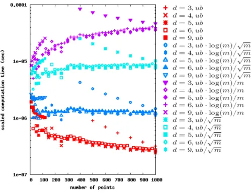
2.3.2 Theoretical vs. Experimental Runtime . . . 53
2.4 Conclusions . . . 58
3 Characteristics of Hypervolume-based EMOA 59 3.1 Concepts and Properties . . . 59
3.2 Convergence Rates . . . 70
3.2.1 Preliminaries . . . 71
3.2.2 SMS-EMOA with Adaptive Reference Point . . . 75
3.2.2.1 (1+1)-SMS-EMOA . . . 75
3.2.2.2 (1,2)-SMS-EMOA . . . 80
3.2.2.3 Limitations of the Approach . . . 81
3.2.3 Population-based SMS-EMOA using Pairwise Comparisons . 84 3.2.4 SMS-EMOA with Fixed Reference Point . . . 87
3.2.5 Other EMOA . . . 91
3.2.6 Conclusions . . . 94
3.3 Optimality of Steady-State-Selection . . . 98
3.3.1 Preliminaries . . . 99
3.3.3 Continuously Differentiable Pareto Fronts . . . 108
3.3.3.1 Theoretical Analysis . . . 108
3.3.3.2 Experimental Analysis on Connected Pareto fronts 110 3.3.4 Conclusions . . . 113
3.4 Performance on Many-Objective Problems . . . 115
3.4.1 Preliminaries . . . 116 3.4.2 Pareto-based EMOA . . . 118 3.4.3 Aggregation-based EMOA . . . 121 3.4.4 Indicator-based EMOA . . . 125 3.4.5 Conclusions . . . 128 3.5 Parameter Tuning . . . 130 3.5.1 Preliminaries . . . 131
3.5.2 Setup of Experimental Analysis . . . 132
3.5.3 DE vs. SBX on CEC 2007 Problems . . . 134
3.5.4 DE vs. SBX on Aerodynamic Problems . . . 137
3.5.5 Conclusions . . . 139
3.6 Hybrid Hypervolume-Gradient Metaheuristic . . . 141
3.6.1 Preliminaries . . . 142
3.6.2 Hypervolume Gradient . . . 144
3.6.3 Gradient-based Pareto Optimization . . . 148
3.6.4 Experiments on SMS-EMOA-Gradient-Hybrid . . . 149 3.6.5 Conclusions . . . 154 4 Summary 157 Nomenclature 161 List of Figures 165 List of Tables 167 List of Algorithms 168 Bibliography 169
Motivation
As known from every day life, people typically do not only have just one wish but several—that may even contradict. In the context of optimization, this means that a solution to a problem shall not just be optimized regarding one goal but fulfill several demands simultaneously. So, considering a real-world problem as a single-objective one does in the best case stem from modesty or priority setting but may be inadequate and a sign of too abstract modeling and over-simplification. The field of multiobjective optimization contrarily provides adequate tools to handle real-world problems canonically by respecting multiple objectives at once.
By the approach of Pareto or vector optimization the solution’s quality is not a single function value but given by a vector containing one value for each objective. As all objectives are treated to be of equal importance, the resolution of a multi-objective problem is a set of Pareto-optimal solutions, containing those solutions which cannot be improved in one objective without worsening in another, thus each representing an optimal compromise. The Pareto-optimal set is typically too large to be captured completely or can practically not be exactly attained in continuous objective spaces. Thus, optimizers can only be expected to achieve an approxima-tion of the Pareto-optimal set. To this end, it is an important task to compare the quality of such approximations. Several quality measures exist, wherein the hypervolume indicator is the most significant and suitable one, making it a key aspect of multiobjective optimization. The hypervolume measures the size of the objective space consisting of worse points than the considered set, so that capturing the objective space up to the optimal set corresponds to its maximization. The space is bounded by a reference point which is a parameter of the hypervolume. The hypervolume calculation is time-consuming since the computation time grows exponentially with the dimension of the objective space.
The hypervolume computation as the core problem of multiobjective optimization is tackled in this thesis by analyzing the hypervolume complexity, giving a simple hypervolume algorithm, and dealing with the choice of its reference point.
Evolutionary multiobjective optimization algorithms (EMOA) developed to state-of-the-art methods for Pareto optimization. Evolutionary algorithms (EA) are
randomized search heuristics that are inspired by the notion of the natural evolution as a process of stepwise improvement through variation and selection. They are especially suitable for complex, badly understood real-world problems since they do not require any problem information such as gradients but handle the problem as a black box. Due to their effectiveness and universal applicability, they gained more and more acceptance in industrial applications, especially the EMOA for multiobjective optimization.
In principle, EMOA can consist of operators developed for single-objective opti-mization, except for the selection. The selection decides about which solutions to keep or to discard for the next iteration. This requires that the solutions are com-parable, which is not directly possible in the multiobjective case since the solutions are vectors. When one solution is better in one and worse in another objective than a second solution, they cannot be sorted. The recent approach is to invoke quality measures to evaluate the current approximation of the EMOA, resulting in the so-called indicator-based EMOA.
Among these algorithms is the SMS-EMOA, where SMS stands for S-metric (a synonym for hypervolume) selection. As it is agreed that an optimizer shall gener-ate an approximation of the optimal set with a high hypervolume value, the idea to directly aspire the hypervolume maximization within the EMOA seems natural and doing this in the selection solves the problem of how to handle incomparable solutions: A solution’s quality is evaluated by its contribution to the hypervol-ume of the current approximation. This is a single-objective problem enabling the solutions to be sortable.
Nowadays, the SMS-EMOA is a popular and accepted algorithm which is in the research community acknowledged by nearly 300 citations (due to Google Scholar (2011)) of the initial conference publication and the journal article, and for example in Germany reflected by its recommendation in the guidelines of the Association of German Engineers (VDI) VDI-Fachbereich Bionik (2011). Yet, although it took just one day to develop SMS-EMOA and it has been competitive right from the start, it is not obvious why and it took years to understand its optimization process.
This thesis is dedicated to the deeper understanding of the optimization process underlying hypervolume-based EMOA like the SMS-EMOA and to specify their performance characteristics.
Overview and Format
The introductory Chapter 1 gives fundamental concepts on a basic level also amend-able for readers unfamiliar with the topic. The two main chapters and each section start with specific and technically detailed preliminaries for the respective subject.
Chapter 2 deals with the calculation of the hypervolume, starting with a com-prehensive overview of its properties including results from literature in simplified notation and additional insights (Sec. 2.1). Our main contributions, the lower bound of the problem complexity and the upper bound as an algorithm are given in the Sections 2.2 and 2.3.
The characteristics of hypervolume-based EMOA are studied in Chapter 3. It focuses on the SMS-EMOA and starts by recapitulating its concept and results of previous studies, next to an overview of other EMOA considered in compari-son (Sec. 3.1). First, the convergence towards the Pareto front is analyzed sepa-rately (Sec. 3.2), followed by a study of the selection behavior on the Pareto front (Sec. 3.3). In Sec. 3.4, the whole process of the SMS-EMOA and other optimizers is benchmarked on problems with many objectives. The performance influence of tuning the parameters—especially the variation—of SMS-EMOA is studied in Sec-tion 3.5. Finally, a hybridizaSec-tion of the SMS-EMOA and a hypervolume gradient technique is presented (Sec. 3.6).
Chapter 2 and each section in Chapter 3 close with a summary of the key results, and a discussion on their impact and remaining open problems as conclusions. The final Chapter 4 recapitulates in a similar way the whole thesis while taking a broader view.
Nearly all results of this dissertation have already been released in publications I (co-)authored. References to these papers are marked with a star (e.g. Beume et al. (2010)∗). Parts of these peer-reviewed publications are reproduced here literally. For precise referencing and complaisant readability, these parts are indicated by blue font and the cited original publication is referenced in the beginning of the respective section. A reference is given at the end of each published theorem, for example as Beume et al. (2010)∗ if the statement has not been changed and by (cf. Beume et al. (2010)∗) in case the result has been altered or extended. For figures and tables, the component’s name in blue font (e.g. Fig. 2.10) indicates that it has been adopted unchanged.
Throughout this thesis the term hypervolume replaces the deprecated synonym S-metric.
For easier readability, vectors are only marked as transposed in case of vector calculations where it is important whether a vector is a row vector or a column vector. A column vector is denoted byxand its transposed row vector byx>. The termsvectororpointare used synonymously. Likewise, we consequently distinguish between sets and multisets in formal statements but often use the term set in descriptive text for convenience. The abbreviations EA and EMOA shall represent the singular as well as the plural form.
List of Underlying Publications
The publications are listed in their order of appearance in this thesis. My contribu-tion to each joint publicacontribu-tion ofk authors can be quantified as a fraction of about
1/k.
1. N. Beume, C. M. Fonseca, M. López-Ibáñez, L. Paquete, and J. Vahrenhold. On the complexity of computing the hypervolume indicator. IEEE Transac-tions on Evolutionary Computation, 13(5):1075–1082, 2009.
The lower bound developed in this paper, conjointly with Carlos M. Fonseca and Jan Vahrenhold, is described in Section 2.2, and a preposed lemma in Section 2.1.
2. N. Beume. S-metric calculation by considering dominated hypervolume as Klee’s measure problem. Evolutionary Computation, 17(4):477–492, 2009. The results are reproduced in Section 2.3.
3. N. Beume, B. Naujoks, and M. Emmerich. SMS-EMOA: Multiobjective selection based on dominated hypervolume. European Journal of Operational Research, 181(3):1653–1669, 2007.
This article summarizes the highlights of our publications Emmerich et al. (2005)∗, Naujoks et al. (2005a)∗, Naujoks et al. (2005b)∗ and is briefly re-viewed in Section 3.1.
4. N. Beume, B. Naujoks, and G. Rudolph. SMS-EMOA: Effektive evolutionäre Mehrzieloptimierung. at-Automatisierungstechnik, 56(7):357–364, 2008. The article is briefly reviewed in Section 3.1. It is an extension of:
N. Beume, B. Naujoks, and G. Rudolph. Mehrkriterielle Optimierung durch evolutionäre Algorithmen mit S-Metrik-Selektion. In R. Mikut and M. Reis-chl, editors, Proc. of the 16. Workshop Computational Intelligence, pages 1– 10. Universitätsverlag Karlsruhe, Karlsruhe, 2006. Young Author Award.
5. N. Beume, M. Laumanns, and G. Rudolph. Convergence rates of (1+1) evolutionary multiobjective algorithms. In R. Schaefer et al., editors, Proc. of the 11th International Conference on Parallel Problem Solving from Nature – PPSN XI: Part I, volume 6238 ofLecture Notes in Computer Science, pages 597–606. Springer, Berlin, 2010. Best Student Paper Award.
The results are contained in Section 3.2.
6. N. Beume, M. Laumanns, and G. Rudolph. Convergence rates of SMS-EMOA on continuous bi-objective problem classes. In H.-G. Beyer and W. B. Langdon, editors, Proc. of the 11th ACM SIGEVO workshop on Foundations
of Genetic Algorithms (FOGA 2011), pages 243–252. ACM, New York, NY, 2011.
The results are as well contained in Section 3.2.
7. N. Beume, B. Naujoks, M. Preuss, G. Rudolph, and T. Wagner. Effects of 1-greedy S-metric-selection on innumerably large pareto fronts. In M. Ehrgott et al., editors, Proc. of the 5th International Conference on Evolutionary Multi-Criterion Optimization (EMO 2009), volume 5467 of Lecture Notes in Computer Science, pages 21–35. Springer, Berlin, 2009.
Section 3.3 is based on this publication.
8. T. Wagner, N. Beume, and B. Naujoks. Pareto-, aggregation-, and indicator-based methods in many-objective optimization. In S. Obayashi et al., editors, Proc. of the 4th International Conference on Evolutionary Multi-Criterion Optimization (EMO 2007), volume 4403 of Lecture Notes in Computer Sci-ence, pages 742–756. Springer, Berlin, 2007.
Section 3.4 is based on this publication.
9. S. Wessing, N. Beume, G. Rudolph, and B. Naujoks. Parameter tuning boosts performance of variation operators in multiobjective optimization. In R. Schaefer et al., editors, Proc. of the 11th International Conference on Parallel Problem Solving from Nature – PPSN XI: Part I, volume 6238 of Lecture Notes in Computer Science, pages 728–737. Springer, Berlin, 2010. Section 3.5 is based on this publication.
10. M. Emmerich, A. Deutz, and N. Beume. Gradient-based/evolutionary relay hybrid for computing pareto front approximations maximizing the S-Metric. In T. Bartz-Beielstein et al., editors, Proc. of the 4th International Work-shop on Hybrid Metaheuristics (HM 2007), volume 4771 ofLecture Notes in Computer Science, pages 140–157. Springer, Berlin, 2007.
The results are reproduced in Section 3.6 and a lemma is preposed to Sec-tion 2.1.
11. P. Koch, O. Kramer, G. Rudolph, and N. Beume. On the hybridization of SMS-EMOA and local search for continuous multiobjective optimization. In F. Rothlauf, editor, Proc. of the 11th Annual conference on Genetic and Evolutionary Computation (GECCO 2009), pages 603–610. ACM, New York, NY, 2009.
The results are briefly reviewed in Section 3.6.
12. T. Voß, N. Beume, G. Rudolph, and C. Igel. Scalarization versus indicator-based selection in multi-objective CMA evolution strategies. In J. Wang
et al., editors, Proc. of the 2008 IEEE Congress on Evolutionary Computa-tion (CEC 2008) within the 2008 IEEE World Congress on ComputaComputa-tional Intelligence, pages 3041–3048. IEEE Press, Piscataway, NJ, 2008.
The results are briefly reviewed in Section 3.6.
Software
The described algorithms are available in several programming languages at:
http://www.hypervolume.org
Acknowledgments
First of all, I would like to express my gratitude to my supervisor Günter Rudolph for sharing his expertise in uncountable professional discussions, his strong interest in my work, and helpful support of this thesis. I thank Christian Igel for agreeing to examine this thesis and his helpful comments. Thanks to my co-authors of the pub-lications that underlie this document for the fruitful cooperations, namely André Deutz, Michael Emmerich, Carlos M. Fonseca, Christian Igel, Patrick Koch, Oliver Kramer, Marco Laumanns, Manuel López-Ibáñez, Boris Naujoks, Luís Paquete, Mike Preuß, Günter Rudolph, Jan Vahrenhold, Thomas Voß, Tobias Wagner, and Simon Wessing, as well as further co-authors of publications not included here. Moreover, I am grateful for the friendly and inspiring atmosphere at the Chair of Algorithm Engineering (LS11). Finally, I heartily thank my beloved husband Thorsten for accompanying and supporting me throughout this work, and for ev-erything else.
The fundamental concepts of the discipline are presented on a basic level amendable to non-familiar readers, referring to subsequent chapters where the knowledge is re-quired and further literature. The basic definitions of multiobjective optimization follow (Sec. 1.1), next to the ideas of how to measure the quality of approximations of the optimal set (Sec. 1.2). Evolutionary algorithms are introduced as suitable optimizers for multiobjective optimization (Sec. 1.3). In Section 1.4, we distin-guish the two computation models used in this work, and describe our approach of experimental test scenarios in Section 1.5.
1.1 Multiobjective Optimization
Multiobjective or multicriteria optimization can be considered as a canonical ap-proach to solve real-world problems. As experienced in every day life, a solution to a problem shall not just be optimized regarding one goal but fulfill several demands. Two main approaches can be distinguished, namely the a prioriand the a posteri-ori approaches. The a priori techniques (cf. Miettinen (1999)) require a weighting of the problem’s objectives prior to the optimization. Summing up the weighted objectives results in a single-objective function with the desired solution as the optimum. Thereby, user preferences can be respected by the optimizer in order to generate a solution with the favored properties. A drawback is that it is usually hard for the user to express her wishes in weights, and to specify the intended ratio before knowing which compromises are possible among objectives. Moreover, not all compromises of objectives are reachable with the described weighting.
Contrarily, a posteriori approaches (cf. Miettinen (1999)) like thevector orPareto optimization1 consider all objectives to be of equal importance, thus all compromise
solutions that cannot be improved in one objective without worsening in another are considered to be optimal, thus resulting in a set of optimal solutions. The opti-mizer approximates the optimal set, so that the user (or decision maker) can decide based on this knowledge which compromise solution fits best to her interests. This approach is used in this thesis, where we deal with the generation of the approxi-mation but not with the decision of a solution. The basic concepts are detailed in the following definitions. For a comprehensive introduction and overview, see e.g. Miettinen (1999), Deb (2001), Coello Coello et al. (2002), or Ehrgott (2005).
1Note that the nomenclature in the literature is ambiguous: it is also common to treat
The following definitions allow us to distinguish between sets and multisets where necessary.
Definition 1.1 Let A = {{a(1), a(2), . . . , a(m)}} denote a multiset of size m, so A may contain copies, i.e., a(i) =a(j), is possible with i=6 j and i, j ∈ {1, . . . , m}, or
otherwise A is a set.
Definition 1.2 The operator set denotes the transformation of a multiset into a set by removing copies, while keeping one element of each subset of equal elements.
We consider unconstrained multiobjective optimization problems in real-valued spaces.
Definition 1.3 An unconstrained multiobjective optimization problem is defined as min
x∈Rn
f(x), with f : Rn →
Rd, f(x) = (f1(x), . . . , fd(x)), fi : Rn → R, i ∈ {1, . . . , n}.
Let the domain of f be denoted as S ⊂ Rn and the co-domain be the multiset
Z ∈ M(Rd) with elements from
Rd.
We notate optimization problems as minimization problems. They can be trans-ferred into equivalent maximization problems since min
x∈Rnf(x) = −maxx∈
Rn{−
f(x)}. The following relations among vectors are applied to relate solutions of multiob-jective problems to each other in order to compare their quality.
Definition 1.4 Let a,b ∈Rd denote twod-dimensional points (or vectors). 1. ab, a weakly dominates b :⇐⇒ ∀i∈ {1, . . . , d}:ai ≤bi 2. a≺b, a dominates b :⇐⇒ ab and a6=b, i.e., ∃i∈ {1, . . . , d}:ai < bi 3. a≺≺b, astrictly dominates b :⇐⇒ ∀i∈ {1, . . . , d}:ai < bi
4. akb, a and b are incomparable:⇐⇒
neither ab nor ba.
5. ab ⇐⇒ ba, analogously for ,
6. ab ⇐⇒ ab is not true, i.e., ba orakb.
a⊀b ⇐⇒ a≺b is not true, i.e., a=b or ba orakb. a 6≺≺b ⇐⇒ a≺≺b is not true, i.e., ab orba orakb. a∦b ⇐⇒ akb is not true, i.e., ab orba.
Lemma 1.5 A hierarchy of dominance relations exists by definition:
a≺≺b ⇒ a≺b ⇒ ab.
The minimal or best elements regarding the Pareto dominance are considered anent to an optimization problem or within sets or multisets.
Definition 1.6 The minimal elements of a multiobjective optimization problem f :S →Z regarding the partial order induced by the Pareto dominance are called Pareto-optimal. Formally, we denote the multiset of optima in the objective space as P F(f)⊆Z as the Pareto front
P F(f) ={{v∈Z | @a∈Z :a≺v}},
and the set of optimizers P S(f)⊆S in the search space as the Pareto set P S(f) ={x∈S |@y∈S :f(y)≺f(x)}={x∈S | f(x)∈P F(f)}.
Definition 1.7 A setA⊂Rdof points that are pairwisely incomparable regarding
the ≺ relation, formally ∀a,b ∈ A : a ⊀ b and b ⊀ a, is called a non-dominated set or an antichain regarding ≺.
A non-dominated multiset can be generated from an arbitrary multisetB ⊂Rd by
removing dominated elements:
ndms(B) = {{b∈B | @a∈B :a≺b}},
and a non-dominated set can be generated by additionally removing copies:
nds(B) =set{{b∈B | @a∈B :a≺b}}.
Note that the termnon-dominated setis commonly used in literature assuming that copies in sets are unlikely in continuous spaces, whereas the term non-dominated multisetis newly introduced here.
The nadir point of a set constitutes of the worst coordinate values in the set, respectively in each dimension. It describes the smallest upper bound of a set, in the sense that it is the point which is weakly dominated by each point of the set and there is no point dominating this one with this property. Analogously the ideal point is the largest lower bound of a multiset, i.e., the point that weakly dominates each element of the multiset. The basic definitions above are illustrated in Fig. 1.1. Definition 1.8 The nadir pointnadof a multisetA∈ M(Rd)describes the small-est upper bound of the multiset:
f1 f2 worse better incomparable incomparable f1 f2 nad(M) ide(M)
Fig. 1.1: Left: Dominance relation of a point in a 2-dimensional space. Right: An example of a Pareto front (blue line), an approximating setM (black points), and its nadir and ideal point.
Definition 1.9 The ideal pointideof a multisetA∈ M(Rd)describes the largest
lower bound of the multiset:
ide(A) := (z1, . . . , zd), with zi = min{ai | a∈A}, i∈ {1, . . . , d}.
Next, the dominance relation among vectors is transferred to sets or multisets of vectors. The relations ≺ and ≺≺ are defined counter-intuitively in literature, so they are omitted here as we do not need them.
Definition 1.10 Let A, B denote two non-empty finite multisets with elements fromRd.
1. A B,A weakly dominatesB :⇐⇒
∀b ∈B :∃a∈A:ab.
2. A kB, A and B are incomparable:⇐⇒
neither AB nor B A. It follows a classification of relations.
Definition 1.11 A binary relation R is a preorder (or quasi-order) over a set M, if ∀a, b, c∈M it fulfills:
1. a R a (reflexivity)
2. a R b ∧ b R c ⇒ a R c (transitivity)
Definition 1.12 A binary relationRis a partial order (or antisymmetric preorder) over a setM, if it is a preorder overM and ∀a, b∈M it fulfills:
Definition 1.13 A binary relation R is a strict (or irreflexive) partial order over a set M, if ∀a, b, c∈M it fulfills transitivity as in Def. 1.11 and:
1. a6R a (irreflexivity)
2. a R b ⇒ b 6R a (asymmetry)
With the definitions above, we characterize the dominance relations among vectors, sets, or multisets to gain a deeper understanding of the relations.
Corollary 1.14 The relation is a partial order over Rd. Proof. ∀a,b,c∈Rd hold with i∈ {1, . . . , d}:
1. Reflexivity: aa, since ∀i:ai ≤ai.
2. Transitivity: ab∧b c⇒ac, since ∀i:ai ≤bi∧bi ≤ci ⇒ai ≤ci.
3. Antisymmetry: ab∧ba⇒a=b, as ∀i:ai ≤bi∧bi ≤ai ⇒ai =bi.
Corollary 1.15 The relations ≺ or ≺≺ form a strict (or irreflexive) partial order over Rd.
Proof. Transitivity holds as in Cor. 1.14.2. ∀a∈Rd hold with i∈ {1, . . . , d}:
1. Irreflexivity: a⊀aand a 6≺≺a.
Since @i:ai < ai, neither a≺anor a≺≺a hold.
2. Asymmetry: a≺b⇒b⊀a and a≺≺b⇒b 6≺≺ a.
Since a ≺ b with ∃i : ai < bi holds, so b ≺ a with ∀i : bi ≤ ai is not true.
Analogously, sincea≺≺b, with∀i:ai < bi holds, sob ≺≺awith∀i:bi < ai
is not true.
Corollary 1.16 The relation is a preorder over subsets fromRd as well as over
M(Rd), the set of all multisets with elements from
Rd, but over both not a partial order.
Proof. 1. and 2. are proved for multisets, holding as well for sets, whereas the negative property 3. is proved for sets, holding as well for multisets. ∀ multisets A, B, C ∈ M(Rd)hold with i∈ {1, . . . , d}:
1. Reflexivity: AA, since ∀a∈A :∃a∈A:aa. 2. Transitivity: A B∧B C ⇒AC.
It holds ∀b∈B :∃a∈A:ab, so∀i :ai ≤bi, and ∀c∈ C:∃b ∈B :b
3. No antisymmetry: AB∧B A 6⇒A=B.
Antisymmetry does not hold for on sets including dominated points. Let A, B ⊂ Rd with B = A∪ {a} and A {a}, a ∈/ A. Then mutually weak
dominance holds while B contains an additional dominated point. As an ad-ditional argument, antisymmetry does not hold foron multisets containing copies. Let A, B ∈ M(Rd) with B = A∪ {a} and a ∈ A. Then mutually
weak dominance holds while the sets are not equal.
Corollary 1.17 The relation is a partial order over the non-dominated sets of
M(Rd).
Proof. The proofs of reflexivity and transitivity are analogous to Cor. 1.16. ∀ multisets A, B, C ∈ M(Rd), thus nds(A), nds(B), nds(C) ⊂ Rd hold with i ∈
{1, . . . , d}:
1. Reflexivity: nds(A)nds(A).
2. Transitivity: nds(A)nds(B)∧nds(B)nds(C) ⇒ nds(A)nds(C). 3. Antisymm.: nds(A)nds(B)∧nds(B)nds(A) ⇒ nds(A) =nds(B).
Proof by contradiction: Assume nds(A) = nds(B) does not hold. Then
∃a ∈ A with a ∈/ B. Since nds(B) nds(A) there ∃b ∈ B : b a with a 6= b. Then, since nds(A) nds(B) there ∃c ∈ A : c b. Due to transitivity with ∀i: ci ≤ bi ≤ai and a 6=c as a6=b, it follows c≺ a. This
contradicts with the definition of nds(A).
1.2 Quality Assessment
To evaluate the quality of an approximation to Pareto-optimal points, the ap-proaching is normally considered in the objective space towards the Pareto front. Approximating the Pareto set is an even more ambitious aim as one point in the objective space may have multiple preimages in the search space so that the Pareto set is larger. It is commonly agreed that the Pareto front approximation is the pri-mary goal, although the Pareto set is as well desired, e.g. to have several different solutions with equal quality to choose from.
The definitions in Section 1.1 allow to relate approximations to each other, e.g. a set that dominates another is a better approximation. Yet, the typical case is that the approximations are incomparable. Since the Pareto dominance is not a total order, not all points are comparable. A point located in the middle of a 2-dimensional objective space dominates 1/4 of it, is dominated by 1/4, and is incomparable to
1/2 of the objective space. So it is comparable with 1/2 of the space, and this fraction decreases exponentially with increasing dimension of the objective space
to 2−d+1 in d dimensions. As the comparability of sets requires the comparability of their elements, approximations are typically incomparable so that the concept of Pareto dominance is insufficient. Yet a quality assessment is desired to evaluate the performance of optimizers. So an ordering is established artificially with the help of quality measures or indicators based on quality aspects additional to the dominance.
A quality measure or indicator is a mapping of a multiset with elements from Rd to R, a definition that leaves arbitrary freedom which quality aspect to represent. The following informal properties are esirable and often demanded from quality indicators, cf. (Deb, 2001, Ch. 8.1).
Axioms 1.18 A quality measure or indicator α : M(Rd) → R shall respect the following aspects.
1. Convergence: The approximation shall minimize the distance to the Pareto front.
2. Diversity: The approximation shall be spread along the whole Pareto front and be well distributed.
3. Cardinality: The size of the approximating set shall be appropriate.
The last point is discussed contrarily. Of course a larger set approximates an infinitely large set better than a smaller. Despite that, it is agreed that the aim of an optimizer is not to generate the whole Pareto front because of too much required resources, but to determine a good representing set.
The indicators we consider are so-called unary measures as they evaluate exactly one set of points. There also exist measures to evaluate two or more sets relative to each other. This has the drawback that the results are not comparable with sets that have not been invoked in that comparison. So, unary measures are more suitable for benchmarks as they enable to comprise earlier or supplementary studies. The total order the quality measures establish shall be conform with the Pareto dominance relations as far as possible. This demand is specified with the terms of completeness and compatibility regarding a relation, cf. Zitzler et al. (2003). Concretely, for a comparable pair of sets with e.g. A B and B A the quality measure shall evaluate the pair such that A is not inferior to B.
Definition 1.19 Let A, B ∈ M(Rd) denote finite multisets. A quality measure
α :A→R is complete regarding a relation R⊆ A×B if: ∀A, B :A R B ⇒α(A)
better than α(B).
The total order induced by the measure shall not contradict with the partial order of the relation. The better set regarding the measure shall as well be better or at least not worse regarding the relation.
Definition 1.20 Let A, B ∈ M(Rd) denote finite multisets. A quality measure α:A→Riscompatibleregarding a relationR⊆A×B if: ∀A, B :AR B ⇐α(A)
better thanα(B). It is weakly compatible regarding R if: ∀A, B :A R B ⇐ α(A)
not worse thanα(B).
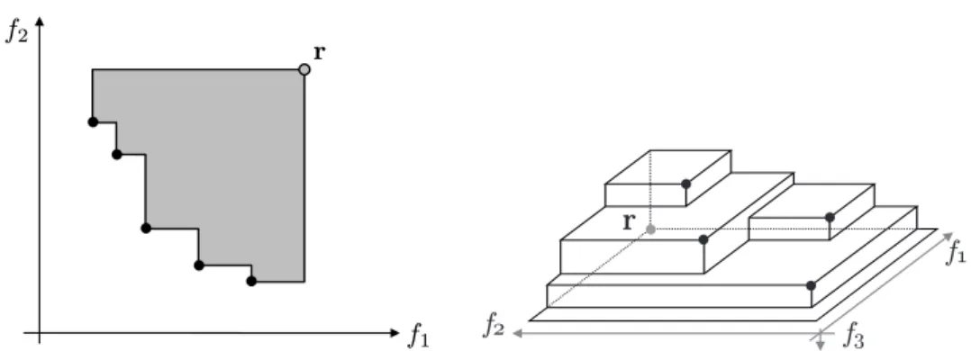
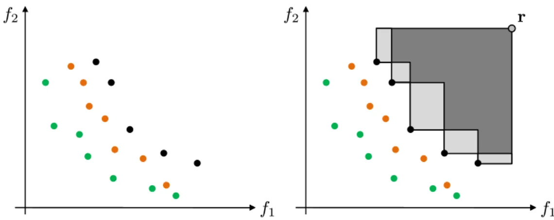
f1 f2 r r f1 f2 f3
Fig. 1.2: Left: Illustration of the 2-dimensional hypervolume (gray area) of a set (black points), bounded by the reference pointr. Right: Hypervolume illustration in a 3-objective space.
Several quality indicators exist and are in usage. Many concentrate either mainly on the diversity or on the convergence. A challenge is to develop measures that evaluate the quality without requiring the knowledge of the Pareto front. Typically convergence measures calculate the distance of the approximation to the Pareto front and are therefore only applicable for test problems where the user is equipped with this knowledge.
Thehypervolume (or S-metric)by Zitzler and Thiele (1998) is the most significant and accepted quality measure in multiobjective research. It measures the size of the space containing points that are dominated by at least one member of the considered set, and is bounded by a reference point (cf. Fig. 1.2). The hypervolume respects all aspects of Axioms 1.18, does not require knowledge of the Pareto front, and is the only known measure which fulfills completeness and compatibility w. r. t. the Pareto dominance relations in the best possible way. A formal definition and detailed properties are given in Chapter 2 followed by the author’s contributions. It is recommended to use several indicators to evaluate the quality of approximation in order to emphasize different aspects. Further indicators used in our experimental analyses are described in Chapter 3. A comprehensive introduction to quality indicators can be found in Knowles et al. (2006), and an in-depth overview of quality indicators and their properties is given in Zitzler et al. (2003) and Zitzler et al. (2008a).
1.3 Evolutionary Algorithms
Evolutionary Algorithms (EA) can be classified according to several methodolo-gies. EA are randomized direct search meta-heuristics for black-box optimization. We explain the terms in an informal way to just sketch the concepts. Search heuris-tics (see e.g. Schwefel (1995)) do not algorithmically calculate an optimal solution but iteratively try valid solutions of unknown quality in order to stepwisely pro-ceed to high quality solutions of the optimization problem. The search space is formally defined so that arbitrary solutions can be generated. Many approaches require information on the gradient of the problem to decide about promising search directions. Contrarily, the term ‘direct’ says that no information about the prob-lem is required except for the function values obtained by point-wise evaluation. This concept suggest these methods for complex problem with unknown proper-ties. Black-box optimization as well expresses this by assuming that nothing is known about the problem so that information can only be gained by executing the black-box with a solution to evaluate the solutions quality. The term ‘heuristic’ says that although thorough strategies are performed, no guaranty of a certain resulting quality of the solutions can be given as this demands assumptions on the problem class. The term ‘meta’ is an addition to express that the algorithms are not limited to a certain problem class but can optimize arbitrary problems. It as well alludes that the methods may conjoin several different techniques, which is also termed ‘hybrid metaheuristic’.
Evolutionary algorithms moreover belong to methods subsumed under the umbrella term Computational Intelligence. These have in common to be inspired by natural archetypes, and also include fuzzy systems, artificial neural networks, swarm intel-ligence, and artificial immune systems (see e.g. Engelbrecht (2007); Konar (2005) for an overview). Evolutionary algorithms are inspired by the Darwinian notion of the evolution as a process of reproduction and selection by survival of the fittest. The strongest individuals adapted best to the environment shall pass their positive characteristics to the next generation by their genetic information so that a species is improved by evolution. Modern EA still base on the concept of iterative im-provements but do not try to imitate biological processes. The nature is used as an valuable source of inspiration, whereas the techniques are then embossed according to the latest knowledge of computer science, mathematics, and statistics.
Historically, evolutionary algorithms had different names due to different commu-nities. Nowadays, evolutionary algorithm (EA) or evolutionary computing (EC) are generic terms subsuming the former directions of genetic algorithms (GA) evo-lutionary strategies (ES) as well as estimation of distributions algorithms (EDA), evolutionary programming (EP), and genetic programming (GP), whereas the three latter differ more in their concepts and are also considered as independent fields. An introduction and overview can be found in Bäck et al. (1997); Eiben and Smith (2007) and recent theoretical results in Auger and Doerr (2011).
initialization evaluation of population parent selection for reproduction variation (recombination/crossover, mutation) selection of succeeding population evaluation of offspring termination condition fulfilled? stop evolution
Fig. 1.3: Operators and evolution cycle of an EA.
Basic Principles
The main components and progression of EA are as follows. The search space has to be encoded such that solutions consist of a vector of parameter values, which is called the representation of solutions. The parameter vector consists of so-called decision variables and is also termed genome according to the biological paradigm. It is, besides the solutions quality and possibly other attributes, stored in a solution or individual. The optimization starts with the initialization of a set of individuals, denoted as population, which is maintained and sought to be optimized throughout the run of the algorithm (cf. Fig. 1.3, Alg. 1.1). The population is mostly initialized uniformly at random in the given search space. The individuals are then evaluated to determine their solution quality or fitness by a black-box solver.
Then a loop or generation is repeated: From the population, individuals are se-lected to become parents of new individuals, a process called parent or mating selection, which is often performed uniformly at random or in a tournament modus where individuals are compared pairwise according to their fitness until ’winners‘ are determined. New individuals or offspring are generated from the parents by probabilistic variation. Recombination or crossover operators combine the infor-mation of typically two individuals to create a new one. Afterwards mutation operators slightly alter the offspring. Crossover is optional, alternatively a copy of a parent is generated and then only changed by mutation.
Having generated and evaluated an offspring population, a subset of the current individuals is discarded to keep only the most promising ones, based on their ob-jective or fitness values. If we discard the whole preceding population, this is called comma selection, denoted by (µ, λ) for a population of size µ and λ offspring per generation. A so-called plus selection filters the best individuals from both old and offspring population, denoted as (µ+λ). In both concepts the population is resized to µ individuals in each generation. After the selection of the subsequent population, the generation is completed. The evolutionary loop has no defined end since the algorithm is not able to verify a solution as optimal. Thus, an aborting
Algorithm 1.1: (µ+1)-EA or (µ+1)-EMOA
1 chooseµ individuals from Rn for initial population P(0), t←0 2 evaluate population P(0)
3 repeat
4 select 2 parents from P(t)
5 create offspringY(t) by recombination of parents 6 mutate offspringY(t)
7 evaluate offspringY(t)
8 select worst individualZ(t) fromP(t)∪Y(t) 9 update population toP(t)←P(t)∪Y(t)\Z(t)
10 t←t+ 1
11 untiltermination criterion fulfilled
condition has to be defined by the user, typically according to resource limitation or the witnessed progress.
Into any component user expertise (if available) may be included in the optimization process to bias the random decisions to known good directions. Seemingly every day, new EA appear, however the state-of-the EA for single-objective optimization are the variants of the CMA-ES by Hansen (2006), Hansen and Ostermeier (2001), and Hansen et al. (2003).
EA for Multiobjective Optimization
Evolutionary Multiobjective Optimization Algorithms (EMOA), also called Multi-objective Evolutionary Algorithms (MOEA), are perfectly qualified for the task of generating an approximation of the Pareto front due to the population concept of optimizing a set of points. In principle, the operators of EA for single-objective optimization can also be used for multiobjective optimization, except for the selec-tion. So the example algorithm in Alg. 1.1 is an EA as well as an EMOA. There is no necessary difference for the variation or other operators considering the search space only, whereas of course dedicated operators may be more effective. Only the selection unavoidably has to deal with the multi-dimensional objective space. Here again, the common concepts—like tournament selection, plus or comma selection etc.—for selecting among the best individuals could be adopted. Yet the problem is the typical absence of a total order among the individuals, so that there is no sorting the selection can base on. So, for EMOA—and as well in modern EA—the fitness value does not simply equate the objective function values, as the fitness in-corporates additional information relative to the current population. Appropriate totally ordered fitness values the selection can base on are in EMOA generated as follows. Many modern EMOA have a two-stage selection process: Firstly, the
indi-viduals are classified as far as possible regarding the dominance or measures based upon it. Examples are non-dominated sorting which performs a kind of ranking based on the transitivity of the dominance, other measures e.g. count the number of dominating individuals. Secondly, an additional measure is applied to enforce an order among the individuals that are still incomparable after the first stage. To this end, diversity measures or quality indicators are used.
The indicator-based EMOA use a quality indicator for the selection at least as a second stage measure. The SMS-EMOA follows this principle by first performing non-dominated sorting on the population and one offspring, and then for the worst subset, the hypervolume is determined and the individual with the least contribu-tion to the hypervolume is denoted as the worst one and is discarded.
The clearly most popular EMOA, NSGA-II by Deb et al. (2002a), is nowadays outdated and no longer recommended, yet it still serves as a reference optimizer in benchmarks, next to the classic algorithm SPEA2 by Zitzler et al. (2002). A modern EMOA is e.g.-MOEA by Deb et al. (2005a), and state-of-the-art EMOA are GDE3 by Kukkonen and Lampinen (2007), or MSOPS and MSOPS-II by Hughes (2003, 2007), as well as the hypervolume-based EMOA, with IBEA by Zitzler and Künzli (2004), MO-CMA-ES by Igel et al. (2007); Voß et al. (2010), and SMS-EMOA by Beume et al. (2007)∗ being the most popular algorithms.
Besides the classic introductions by Deb (2001) or Coello Coello et al. (2002), an overview of modern EMOA and related techniques can be found in Abraham and Goldberg (2005), Knowles et al. (2007), Branke et al. (2008), and recent theoretical insights in Brockhoff (2010b). The EMOA invoked in this thesis are described in Chapter 3, especially detailing the SMS-EMOA and its characteristics.
1.4 Computation Models
Standard Algorithmic ModelThe computation model we consider for the hypervolume calculation in Chapter 2 is the standard model for algorithmic complexity, i.e., also for computational ge-ometry, which is the context we consider the hypervolume in. The calculation time is measured as the number of elementary calculation steps. All steps are assumed to have equal costs (uniform cost model) and we do neither consider space nor resources for communication in distributed systems. An algorithm is considered as a bounded-degree algebraic decision tree that is traversed depending on the input. For a more in-depth exposition, see e.g. Preparata and Shamos (1988, Sec. 1.4). Runtimes are given w. r. t. the size of a set of vectorsm, without the dimension of the vectorsd, assuming d is a constant, i.e., d=O(1) w. r. t.m.
This model is as well used to express the computational resources of an evolutionary algorithm per generation without counting the function evaluations.
Model for Black-Box Optimization
For black-box optimization, a dedicated complexity measure, theblack-box complex-ity, has been developed to express optimization times required to solve a problem class by means of a randomized direct search heuristic. It is assumed that the operations of an algorithm are neglectable compared to the time required for a function evaluation of a real-world problem. Hence, the black-box complexity only gives the number of function evaluations until an optimal function value is found. See Wegener (2005, Ch. 9.) for exact definitions and a more in-depth exposition. In theory on evolutionary algorithms for single-objective optimization, this mea-sure is common practice. As usually, upper bounds for the complexity of a problem are gained by algorithms that solve the problem in that time. It depends on the problem and the optimizer how sound the measure actually is. In multiobjec-tive optimization, the black-box complexity is not necessarily suitable since the calculations of an evolutionary algorithm may be more demanding, e.g. due to hypervolume calculation, so that their resources only fall behind time-consuming function evaluations.
In Chapter 3 we state the runtime of algorithms as resources per generation w. r. t. the standard algorithmic model, and optimization times in black-box complexity.
1.5 Experimental Analyses
Experimental StudiesExperimental studies are a research discipline with a documented tradition of hun-dreds of years, and are more or less the only approach in natural sciences. It could be surmised that computer experiments as not necessary due to the mathematical-based system and algorithms. However, the resulting random processes are far too complex to calculate exactly what is happening. As current theoretical tools are insufficient to answer many relevant research questions, experiments are the only ways to gain insights. Moreover, they are also used to validate that mathematically calculated facts can also be observed when actually running the algorithms, which is not evidently since theoretical analyses as well make assumptions to abstract from reality.
In this work we perform experiments in order to experience how well the theoretical bound of the runtime fits with the real runtime of the hypervolume algorithms in Section 2.3.2. When studying the EMOA in Chapter 3, rigorous analyses are per-formed as far as possible, but the processes are often too complex for current tools, so that experimental studies are performed instead. An overview of state-of-the-art methods of experimental analyses is given in Bartz-Beielstein et al. (2010a). For the documentation of experiments, we mainly follow Preuss (2007), which formu-lates the application of common guidelines of experiments in natural sciences to
computer experiments in the area of evolutionary computation. Tests on statistical significance are performed when it seems necessary in order to validate the results. Academic Test Problems
To benchmark and study certain aspects of EMOA, academic test problems are used. These have the advantage that the problem is well understood and the optima are known as it has been designed clearly structured. They shall represent typical characteristics of real-world problems paradigmatically. In our studies, the test set is respectively chosen according to the posed research question, and with popular test problems in order to establish comparability with similar studies. Note that all problem functions are real-valued and to be minimized.
The ZDT family by Zitzler et al. (2000) comprises 2-objective continuous func-tions, the discrete ZDT5 is excluded here like in most studies from literature. The Pareto front of ZDT1 is convex, ZDT2’s is concave, ZDT3’s consists of five convex parts. ZDT4 has the same Pareto front as ZDT1 but the functions are multimodal. The Pareto front of ZDT6 is a subset of ZDT2’s and the points are distributed asymmetrically. The Pareto set is equal for all ZDT function, with all except the first decision variable equaling zero. The problem family is often used for an initial benchmark of a new optimizer; we apply it in Sections 3.3–3.6.
The DTLZ function family by Deb et al. (2002b) is another popular problem set with scalable number of objectives. Like the ZDT problems, they contain multi-modal problems based on sine and cosine functions. DTLZ1 has a linear Pareto front (e.g. a plane in case of three objectives) and DTLZ2 and DTLZ3 have the same convex Pareto front, more precisely a section of a hypersphere. The runtime of hypervolume algorithms is benchmarked on subsets of the linear and convex DTLZ Pareto fronts (Section 2.3.2). To study and benchmark EMOA, the DTLZ problems and variations of it are applied in Sections 3.3–3.5.
Moreover, other test problems as well as a real-world problem are used in our studies, specified in the respective sections, including the test suite of the CEC 2007 competition, organized by Huang et al. (2007), for the study in Section 3.5. Parameter Handling
Undoubtedly, different optimizers perform different on certain problem classes. Since meta-heuristics, such as EA, are equipped with several parameters that allow to change their behavior, an EA or EMOA can be seen as a plurality of algorithms and the choice of parameter values deserves a closer look.
Two major forms of parameter settings are to be distinguished: parameter control and parameter tuning. Parameter control deals with the handling of parameter values within the EA during its execution. The main concepts are static or adaptive operation, thereby especially dynamic over time or self-adaptive subjected to the evolution process (see Michalewicz et al. (2007) for an overview).
Parameter tuning is the process of finding good values for the external parameters that are set before the algorithm starts (see Bartz-Beielstein et al. (2010a) for an overview of tuning methods). These may function as the initial values of internal adaptive parameter control methods. Finding the best parameterized EA for a problem is an optimization problem by itself. Yet, the goal of the optimization process is not obvious and naturally a multiobjective problem, while demands are e.g. fast progress and convergence to a global optimum. Further requirements arise from the stochasticity of EA, e.g. low variance and high reliability of the results’ qualities. We deal with parameter tuning in Section 3.5.
Calculating the dominated hypervolume is a core problem in multi-objective opti-mization as it is the standard quality measure to evaluate approximations of the Pareto front. After an overview of the problem’s properties, we deal with the com-putational resources required for the hypervolume calculation. Taking the view of computational geometry, the best known lower bound is proved with tools of complexity theory (Sec. 2.2, Beume et al. (2009a)∗). By algorithm engineering, we derive a simple algorithm realizing a hardly worse upper bound than the best known one (Sec. 2.3, Beume (2009)∗).
2.1 Problem Properties
The hypervolume is a unary quality measure that maps a set to a scalar value. This way, an arbitrary number of sets can be compared using the order induced by the hypervolume values. To simplify matters, we consider one or two sets in the following.
After providing basic definitions, we survey properties in simple notation with formal proofs. An emphasis is the relation of the preorder of the dominance relation and the total order according to the hypervolume. The choice of the reference point and its influence are discussed. Results for the distribution of points within a set of maximal hypervolume are presented detailing our contribution for linear Pareto fronts. We give an overview of exact as well as of approximation algorithms. Basic Definitions
The dominated hypervolume describes the size of the space dominated by a set— or more general a multiset—of points. It has first been suggested by Zitzler and Thiele (1998) for performance assessment.
Definition 2.1 LetM ={{v(1),v(2), . . . ,v(m)}} ∈ M(
Rd), d ≥2, m ∈N be a fi-nite multiset, andr∈Rdindicate the reference point. Thedominated hypervolume
(or S-metric) is defined as the quantity
H(M,r) :=Leb {u∈Rd | ∃v∈M :vur} =Leb m [ i=1 [v(i),r] ! . (2.1)
Leb denotes the Lebesgue measure in Rd. The d-dimensional interval [v(i),r] de-scribes the hypercuboid spanned byv(i) and r, indicating the space dominated by
v(i) and bounded by r. In the following, we denote H
s(M,r) := {u ∈ Rd | ∃v ∈
M :vur}
An illustration of the 2-dimensional dominated hypervolume is given in Fig. 2.1 (left). For convenience, we use the popular term hypervolume in the following for dominated hypervolume. The older term S-metric is misleading as the measure is not a metric in the mathematical sense. In the context of multiobjective optimiza-tion, the hypervolume is sought to be maximized.
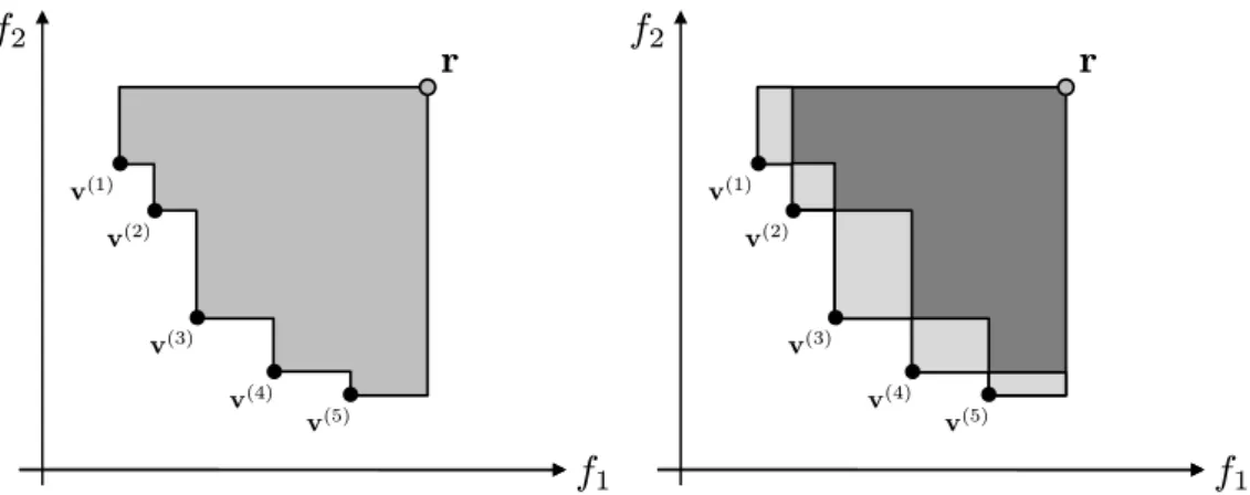
f1 f2 r v(2) v(1) v(3) v(4) v(5) f1 f2 r v(2) v(1) v(3) v(4) v(5)
Fig. 2.1: Left: Illustration of the 2-dimensional hypervolume (gray area) of a set (black points), bounded by the reference pointr. The axesf1, f2 indicate our notion of the 2-dimensional space as the image of a multiobjective problem. Right: The hypervolume contribution of each point is indicated in light gray.
More general definitions of the hypervolume exist, which we do not use here but briefly mention. Instead of one reference point, a reference set can be used to bound the dominated space (cf. Zitzler et al. (2010)). Zitzler et al. (2007) introduced the weighted hypervolume by using a weight distribution to emphasize certain regions of the objective space and thereby realize user preferences. They showed that the weighted hypervolume indicator has the same properties w. r. t. the dominance relation as the original one.
In order to optimize the composition of a set, it is desirable to quantify the value of a single point within that set. To this end, we define the hypervolume contribution of a point to a set as the hypervolume that is exclusively dominated by that single point and thus gets lost when the point is excluded from the set (Fig. 2.1, right). Points with higher hypervolume contribution are preferred over others in the set. Note that the hypervolume contribution is typically calculated w. r. t. a set of non-dominated points. Dominated points or copies in multisets have a contribution of zero but they may reduce the contribution of non-dominated points by sharing a region with them which is then not associated as their exclusive contribution.
Definition 2.2 The hypervolume contribution of the point v∈ M to the hyper-volume of the multiset M ∈ M(Rd) is defined as
H(v, M,r) =H(M,r)−H(M \ {v},r).
Throughout this section it becomes obvious that the hypervolume respects the Ax-ioms 1.18. Points closer to the Pareto front have a higher hypervolume, the hyper-volume of a set increases with additional non-dominated points, so that spreading along the whole Pareto front gets rewarded. Next, we present basic properties of the hypervolume.
Corollary 2.3 LetA, B ∈ M(Rd)be finite multisets. Then,∀A, B,∀v∈
Rd,∀r∈ Rd holds: 1. H(A,r) = 0 ⇐⇒ 6 ∃a∈A:a≺≺r 2. H(A,r)>0 ⇐⇒ ∃a∈A:a≺≺r 3. H(v, A,r) = 0 ⇐⇒ v 6≺≺r or∃a∈A:av 4. H(v, A,r)>0 ⇐⇒ v≺≺r and @a∈A:av
5. Sets with higher hypervolume are preferred over other sets.
6. Points with higher hypervolume contribution are preferred over others in the set.
7. Let M be a set of elements from the co-domain Z ⊂ Rd of a multiobjec-tive optimization problem f : Rn →
Rd. The hypervolume of the set M is maximal among the subsets of Z iff it contains the Pareto front of f.
Proof. The hypervolume as well as the hypervolume contribution are either positive or zero; negative values are not defined.
1., 2.: The hypervolume is positive iff there is at least one point that strictly dominates the reference point. This implies that the hypercuboid spanned by the point and the reference point is full-dimensional. Weaker forms of dominance are not sufficient as they allow equal coordinate values of both points which leads to a hypervolume of zero.
3., 4.: The hypervolume contribution of a pointvis positive iffvstrictly dominates the reference point (for the same reason as in 2.), and v is not weakly dominated by any point of A. For all points in or on the boundary of the space dominated by A holds that they are at least weakly dominated by one point ofA. Thusv indeed lies outside this area, so there is a portion of hypervolume dominated byvbut not dominated by any other point inA, and it is full-dimensional. Formally, the point can be worsened in each dimension byε >0(sufficiently small) to v0. For v0 holds v ≺≺v0 ≺≺r, and @a∈ A,a6=v :a v0. The hypervolume contribution of v is
the Lebesgue measure of the set of these v0.
Otherwise, the hypervolume contribution is zero (4.).
5., 6.: Regarding the hypervolume and the hypervolume contribution higher values are better.
7.: See Fleischer (2003, Theorem 1.) for a proof. The fact also becomes evident in the proof of Theorem 2.4.4.
Ordering according to the Hypervolume
As a quality measure, the hypervolume creates a total order among sets which are only preordered regarding the Pareto dominance relation. The implications below directly follow from the fact that the dominated space of A includes B, if A B. Intuitively, the implications mean that the total order induced by the hypervolume does not contradict with the preorder of the dominance relation, and whenever sets are comparable regarding the dominance relation, the hypervolume indicates this. The following collection of characteristics is partly redundant in the sense that some observation follow from others, yet it seems worthwhile to present facts from different points of view.
Theorem 2.4 Let the dominance relation induce a preorder and the hyper-volume H(·,r) induce a total order among the finite non-empty multisets A, B ∈
M(Rd). Then,∀A, B,∀b ∈ Rd,∀r∈Rd holds: 1. A =B ⇒ H(A,r) =H(B,r) 2. A B ⇒ H(A,r)≥H(B,r) 3. A {b} ⇒ H(A∪ {b},r) =H(A,r) 4. A {b} and b≺≺r ⇒ H(A∪ {b},r)> H(A,r)
5. For all sets A, B of mutually incomparable points:
A B and A6=B ⇒ ∀r: (nad(A∪B)≺≺r) :H(A,r)> H(B,r)
6. A B and B A ⇒ ∀r: (nad(A∪B)≺≺r) :H(A,r)> H(B,r)
7. B A, i.e., (A B∧A6=B)∨AkB ⇐ ∃r∈Rd:H(A,r)> H(B,r)
8. A B and B A ⇐ ∀r: (∃v∈A∪B :v≺≺r) :H(A,r)> H(B,r)
Proof. 1.: Equal sets of course yield equal hypervolume values, as obvious by replacing A byB, whereas this does not hold the other way round.
2.: A B implies ∀b ∈ B : b ∈ Hs(A,r), so H(A,r) cannot be smaller than
H(B,r).
3. The implication says that a dominated point does not add anything to the hypervolume of a set. The left hand side implies that b either lies inside the
hypervolume of A (b ∈ Hs(A,r)), or b is outside such that it does not strictly
dominate the reference point (b 6≺≺ r). In both cases, b does not have a positive contribution toA (cf. Corollary 2.3.3.).
4. A {b} means that @a ∈ A : a b. This combined with b ≺≺ r is the condition for a positive contribution to a set (cf. Corollary 2.3.4.). Thereby b has a positive contribution to A∪ {b} so the hypervolume of this set is larger than that of A. This property allows for a proof of Corollary 2.3.7.: The hypervolume of a set can be improved as long as there is a non-dominated point to include. Therefore the Pareto front is the set with the maximal hypervolume among all sets of solutions of a multiobjective problem.
5. A B implies H(A,r) ≥ H(B,r) (cf. 2.). A 6= B implies ∃a ∈ A : a ∈/ B. This ahas a positive contribution to A, if Corollary 2.3.4 is fulfilled. This positive contribution added to the hypervolume of A makes the hypervolume of A indeed larger than the hypervolume of B. Given the preconditions Corollary 2.3.4 is automatically fulfilled, since a is neither a copy, nor dominated within A, and a≺≺r. With toned down additional precondition, 5. reads:
AB and nds(A)=6 nds(B) ⇒ ∀r with nad(A∪B)≺≺r:H(A,r)> H(B,r). 6. According to the proof of 5., 6. holds when the non-dominated subsets ofAand B are different. This is the case for A B∧B A.
7. B A implies ∀a ∈ A : ∃b ∈ B : b a and so A ⊆ Hs(B,r) causing
H(A,r) ≤ H(B,r) (cf. 2.). This contradicts with the right hand side, so, the opposite must be true. Since 2. holds for all reference points, it suffices to observe H(A,r)> H(B,r)for one reference point to conclude a contradiction.
8. If A B is not true, then ∃b ∈ B : @a ∈ A : a b. Choose the reference point such that it is strictly dominated by this b but not by A: ri = bi +ε for
i = 1, . . . , d and ε > 0 sufficiently small. Then H(B,r) > 0 while H(A,r) = 0. This contradicts with the right hand side, so the opposite must be true. B A implies H(B,r) ≥ H(A,r) due to 2. This contradicts with the right hand side, hence B A holds.
Zitzler et al. (2003) observed 5. and 7. (with less precise specification of the ref-erence point), whereas 5. is named .-completeness, and 7. 7-compatibility (cf. Definition 1.19, 1.20). In Zitzler et al. (2008a), a property resembling 5. is named strict monotonicity. Zitzler et al. (2010, Th. 3.2) term the hypervolume a refine-ment of the dominance relation due to a property resembling 5. (cf. Zitzler et al. (2010, Th. 3.1)). They observed 3. and 4. (cf. (Zitzler et al., 2010, Th. 3.2)) and showed that both in tandem imply 5.
The hypervolume and its variations are the only unary indicators that feature both property 5. and 7. (cf. Zitzler et al. (2007)). Implication 7. cannot be stronger as proved in (Zitzler et al., 2003, Th. 1). Intuitively, it is clear that from a greater hypervolume value, it cannot be followed that the sets are comparable regarding the dominance relation. This would erase the case of incomparability and make the dominance relation a total order, which is obviously not true.
The following lemma says that for two points, their ordering regarding the hy-pervolume is always equivalent to their ordering according to their hyhy-pervolume contribution when combined to a set (cf. Fig. 2.2). This lemma is used in Section 3.2 and has been described informally in Beume et al. (2011)∗.
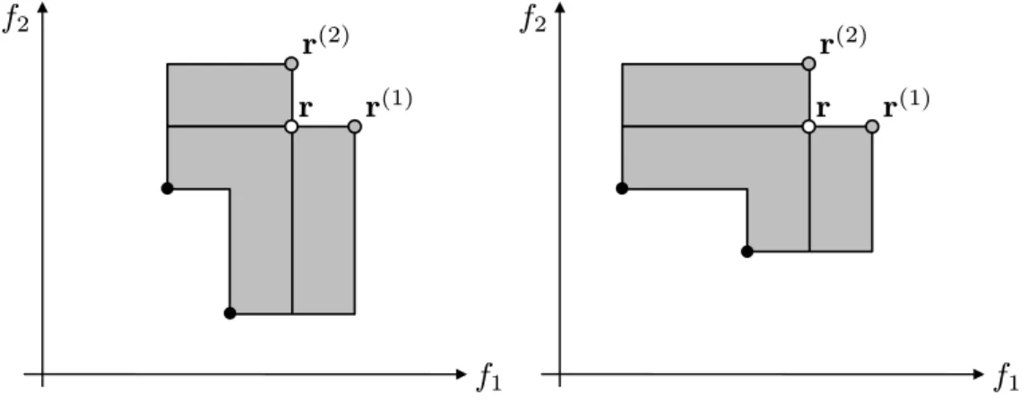
f1 f2
a
b
r
Fig. 2.2: The light gray rectangles depict the hypervolume contribution of the points. The dark gray area is dominated by both points, so its value added to each contri-bution results in the absolute hypervolume of each point. The order induced by both measures is equal.
Lemma 2.5 Leta,b∈Rd. Then ∀d≥2,r∈
Rd with nad(a,b)≺≺r holds: H(a,{a,b},r)•H(b,{a,b},r) ⇐⇒ H({a},r)•H({b},r),
with •being the same relation out of {<, >,=}. (Beume et al. (2011)∗).
Proof. The hypervolume dominated by two points consists of the points’ con-tributions and a part dominated by both points (Fig. 2.2). The hypervolume of each point is equivalent to its hypervolume contribution plus the hypervol-ume dominated by both points. Since this value is equal for both points, it does not affect the order of the points induced by their contributions. Formally, we distinguish three cases: (i) Let a = b. Then H({a},r) = H({b},r) and H(a,{a,b},r) =H(b,{a,b},r) = 0. (ii) Let a≺b. Then H({a},r)> H({b},r)
asb∈Hs({a},r)andH(a,{a,b},r)> H(b,{a,b},r) = 0. (iii) Letakbwitha1 <
b1 anda2 > b2. Withq:= (r1−b1)(r2−a2), thenH({a},r) = (b1−a1)(r2−a2)+q=
H(a,{a,b},r)+qandH({b},r) = (r1−b1)(a2−b2)+q =H(b,{a,b},r)+q. Thus
H({a},r)> H({b},r) ⇐⇒ H(a,{a,b},r)> H(b,{a,b},r), and analogously for the other relations and vice versa roles of aand b.
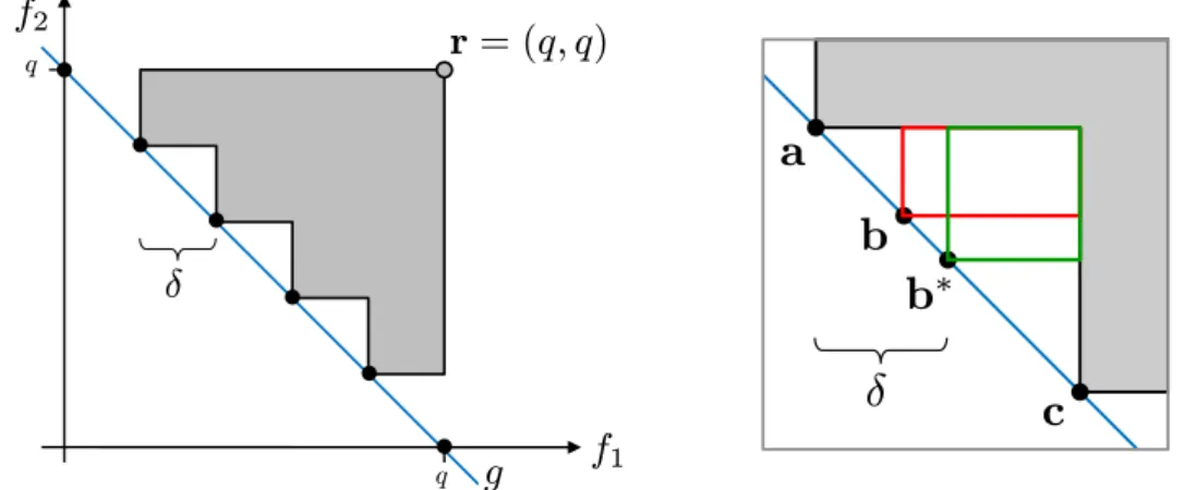
Choice of the Reference Point
The ranking of sets according to the hypervolume allows for their comparison. To make this comparison fair, it is common practice to choose the same reference point