All Faculty Scholarship for the College of the
Sciences College of the Sciences
4-2019
Weighted Random Search for Hyperparameter Optimization
Weighted Random Search for Hyperparameter Optimization
Adrian-Cǎtǎlin FloreaTransilvania University of Braşov
Rǎzvan Andonie
Central Washington University
Follow this and additional works at: https://digitalcommons.cwu.edu/cotsfac Part of the Computer Sciences Commons
Recommended Citation Recommended Citation
Florea, Adrian-Cǎtǎlin and Andonie, Rǎzvan, "Weighted Random Search for Hyperparameter Optimization" (2019). All Faculty Scholarship for the College of the Sciences. 110.
https://digitalcommons.cwu.edu/cotsfac/110
This Article is brought to you for free and open access by the College of the Sciences at ScholarWorks@CWU. It has been accepted for inclusion in All Faculty Scholarship for the College of the Sciences by an authorized administrator of ScholarWorks@CWU. For more information, please contact [email protected].
Weighted Random Search for Hyperparameter Optimization
A.C. Florea, R. Andonie Adrian-Cătălin Florea*
Department of Electronics and Computers Transilvania University of Braşov, Romania *Corresponding author: [email protected]
Răzvan Andonie
Department of Computer Science Central Washington University, USA [email protected]
Abstract: We introduce an improved version of Random Search (RS), used here for hyperparameter optimization of machine learning algorithms. Unlike the standard RS, which generates for each trial new values for all hyperparameters, we generate new values for each hyperparameter with a probability of change. The intuition behind our approach is that a value that already triggered a good result is a good candidate for the next step, and should be tested in new combinations of hyperparameter values. Within the same computational budget, our method yields better results than the standard RS. Our theoretical results prove this statement. We test our method on a variation of one of the most commonly used objective function for this class of problems (the Grievank function) and for the hyperparameter optimization of a deep learning CNN architecture. Our results can be generalized to any optimization problem defined on a discrete domain.
Keywords:Hyperparameter optimization, random search, deep learning, convolu-tional neural network.
1
Introduction
The vast majority of machine learning algorithms involve two different sets of parameters:
the training parameters and the meta-parameters (also known as hyperparameters). While the
training parameters are learned during the training phase, the values of the hyperparameters have to be specified before the learning phase. For instance, the hyperparameters of neural networks typically specify the architecture of the network (number and type of layers, number and type of nodes, etc).
Determining the optimal combination of hyperparameter values leading to the best gen-eralization performance can be done through repeated training and evaluation sessions, trying different combinations of hyperparameter values. We call each training + evaluation process for
one combination of hyperparameter values atrial. Each trial is computationally expensive, since
it involves re-training the model. In addition, the number of trials increases generally exponen-tial with the number of hyperparameters. Therefore, it is important to reduce the number or trials [9]. This can be done by both reducing the number of hyperparameters and reducing the value range of each hyperparameter, while still maximizing the probability to hit the optimal combination [2,3].
Various hyperparameter optimization methods were developed during the years, ranging
from very simple ones, such as Grid Search (GS) and manual tuning [14, 20, 28]1, to highly
1
https://github.com/jaak-s/nips2014-survey - 82 out of 86 optimization related papers presented at the NIPS 2014 conference used GS.
elaborated techniques: Nelder-Mead [1, 24], simulated annealing [17], evolutionary algorithms [12], Bayesian methods [32], etc.
Recently, there has been significant interest in the area of hyperparameter optimization, especially since the rise of deep learning which puts a lot of pressure on the existing techniques due to the very large number of hyperparameters involved and the significant training time needed for such architectures. The focus in hyperparameter optimizations presently oscillates between introducing more sophisticated techniques (Sequential Model-Based Global Optimization [2], reinforcement learning [34,35], etc) and various attempts to optimize existing simple techniques. RS falls into the category of simple algorithms [2, 3]. Making use of the same computa-tional budget, RS generally yields better results than GS or more complicated hyperparameter optimization methods [2]. Especially in higher dimensional spaces, the computation resources required by RS methods are significantly lower than for GS [21]. RS consists in drawing sam-ples from the parameter space following a particular distribution for each of the parameters. Each trial is drawn and evaluated independently from the others, which makes RS a very good candidate for parallel implementations.
Some recent attempts to optimize the RS algorithm are: Li’s et al. Hyperband [22], which
speeds up RS through adaptive resource allocation and early-stopping; Domhanet al.[8], which
have developed a probabilistic model to mimic early termination of sub-optimal candidate; and
Floreaet al.[9], where we introduced a dynamically computed stopping criterion for RS, reducing
the number of trials without reducing the generalization performance.
There are various software libraries implementing hyperparameter optimization methods. Hyperopt [4] and Optunity [7] are currently two of the most advanced standalone packages. Bayesian techniques are implemented by packages like BayesianOptimization [29] and pyGPGO [27]. Some of the best known general purpose machine learning software libraries also provide hyperparameter optimization: LIBSVM [5] and scikit-learn [26] come with their own implemen-tation of GS, with scikit-learn also offering support for RS. Auto-WEKA [18], built on top of Weka [11] is able to perform GS, RS, and Bayesian optimization.
Lately, commercial cloud-based services started to offer hyperparameter optimization capa-bilities. Among them we count Google HyperTune [38], BigML’s OptiML [36], and SigOpt [40]. All of them support mixed search domains, SigOpt being able to handle objective, multi-solution, constraint (linear and black-box), and parallel optimization.
In this context, our contribution is an improved version of the RS method, the Weighted
Random Search (WRS) method. Unlike the standard RS, which generates for each trial new
values for all hyperparameters, we generate new values for each hyperparameter with a
prob-ability of change p and we use the best value found so far for that particular hyperparameter
with probability 1−p, where p is proportional to the hyperparameter’s relative importance in
the variation of the objective function. The intuition behind our approach is that a value that already triggered a good result is a good candidate for a new trial and should be tested in new combinations of hyperparameter values.
For the same number of trials, the WRS algorithm produces significantly better results than RS. We obtained theoretical results which prove this statement. We tested our algorithm on a slightly modified version of one of the most commonly used objective function for this class of problems - the Grievank [10] function, as well as for the hyperparameter optimization of a deep learning CNN architecture using the CIFAR-10 [37] dataset.
Unlike our previous work on RS optimization [9], where our focus was on the dynamic reduc-tion of the number of trials, the focus of the WRS method is the optimizareduc-tion of the classificareduc-tion (prediction) performance within the same computational budget. The two approaches make use of different optimization techniques.
Section 3 describes theoretical results and the convergence of WRS. Sections 4 and 5 contain experimental results. The paper is concluded with Section 6.
2
The WRS method
We first present the generic intuitive description of the WRS algorithm, which is the core of our contribution. Technical details will be provided later.
The standard RS technique [2] generates a new multi-dimensional sample at each stepk, with
new random values for each of the sample’s dimensions - features, in our case -Xk ={xki}, i=
1, . . . , d, where xi is generated according to a probability distribution Pi(x), i= 1, . . . , d, and d
is the number of dimensions.
WRS is an improved version of RS, designed for hyperparameter optimization. It assigns probabilities of change pi, i = 1, . . . , d to each dimension. For each dimensioni, after a certain
number of stepski, instead of always generating a new value, we generate it with probabilitypi
and use the best value known so far with probability1−pi.
The intuition behind the proposed algorithm is that after already fixing d0 (1 < d0 < d)
values, each d-dimensional optimization problem reduces itself to a d−d0 dimensional one. In
the context of thisd−d0 dimensional problem, choosing a set of values that already performed
well for the remaining dimensions might prove more fruitful than choosing somed−d0 random
values. In order to avoid getting stuck in a local optimum, instead of setting a hard boundary between choosing the best combination of values found so far or generating new random samples, we assign probabilities of change for each dimension of the search space.
WRS has two phases. In the first phase, it runs the RS for a predefined number of trials
and allows: a) to identify the best combination of values so far; and b) to give enough input on
the importance of each dimension in the optimization process. The second phase considers the probabilities of change and generates the candidate values according to them. Between these two phases, we run one instance of fANOVA [15], in order to determine the importance of each dimension with respect to the objective function. Intuitively, the most important dimension (the dimension that yields the largest variation of the objective function) is the one that should change most frequently, to cover as much of the variation range as possible. For a dimension with small variation of the objective function, it might be more efficient to keep a certain temporary optimum value once this has been identified.
A step of the WRS algorithm applied to function maximization is described by Algorithm
1, whereas the entire method is detailed in Algorithm 2. F is the objective function, the value
F(X) has to be computed for each argument, Xk is the best argument at iteration k, whereas
N is the total number of iterations.
At each step of Algorithm 2, at least one dimension will change, hence we always choose at least one of thepi probabilities to be equal to one. For the other probabilities, any value in(0,1]
is valid. If all values are one, then we are in the case of RS.
Besides a way to compute the objective function, Algorithm 1 requires only the combination
of values that yields the bestF(X) value obtained so far and the probability of change for each
dimension. The current optimal value of the objective function can be made optional, since the comparison can be done outside of Algorithm 1. Algorithm 2 coordinates the sequence of
the described steps and calls Algorithm 1 in a loop, until the maximum number of trials N is
Algorithm 1 A WRS Step - Objective Function Maximization Input: F; (Xk,F(Xk)); pi, ki, Pi(x), i= 1, . . . , d
Output: (Xk+1, F(Xk+1))
1: Randomly generatep, uniform in (0,1)
2: fori= 1 to ddo
3: if (pi≥por k≤ki)then
4: // either the probability condition is met or more samples are needed
5: Generate xki+1 according toPi(x)
6: else
7: xki+1=xki
8: end if
9: end for
10: // usually this is the most time consuming step
11: ComputeF(Xk+1) 12: if F(Xk+1)≥F(Xk) then 13: return(Xk+1, F(Xk+1)) 14: else 15: return(Xk, F(Xk)) 16: end if
Algorithm 2 WRS - Objective Function Maximization Input: F;N;Pi(x), i= 1, . . . , d
Output: (XN, F(XN)) 1: // Phase 1 - Run RS
2: fork= 1 to N0 < N do
3: Perform RS step, compute(Xk, F(Xk))
4: end for
5: // Intermediate phase, determine input for WRS
6: Determine the probability of changepi, i= 1, . . . , d
7: Determine the minimum number of required valueski, i= 1, . . . , d
8: // Phase 2 - Run WRS
9: fork=N0+ 1toN do
10: Perform WRS Step described in Algorithm 1, compute(Xk, F(Xk))
11: end for
3
Theoretical aspects and convergence
We aim to analyze the theoretical convergence of Algorithm 2 and compare it to the RS method. Similar to GS and RS, we make the assumption that there is no statistical correlation between the variables of the objective function (hyperparameters). To make explanations more intuitive, we first discuss the two-dimensional case, and then generalize for the multi-dimensional case. We will also define what we consider "a set of good candidate values" for pi and ki, i = 1, . . . , d(used in steps 6 & 7, Algorithm 2). We denote byn≥1the number of iterations (steps)
for both RS and WRS.
3.1 Two-dimensional case
In the two-dimensional case (d= 2), we aim to maximize a functionF :S1×S2 →R, where
S1 and S2 are countable sets. We define as global optimum the pointX∗(x1∗, x∗2), with x∗1 ∈S1
and x∗2 ∈ S2, so that F(X∗) ≥ F(X),∀X ∈ S1 ×S2. pi, ki,(i = 1,2) are the probabilities of
change, respectively, the required number of distinct values for xi, as previously defined. |Si|is
the cardinality ofSi, i= 1,2. We denote bypRS:nandpW RS:nthe probability for RS, respectively
WRS, to reach the global optimum afternsteps.
The following theorem establishes that, in the two-dimensional case we can choose k2 so
that
pW RS:n≥pRS:n (1)
Theorem 1. For any function F :S1×S2 →R there existsk2, so that pW RS:n≥pRS:n.
Proof: We consider the case of maximizing function F, and choose the arguments in the
de-creasing order of their probabilities of change. Since the value for one dimension always changes,
we have p1 = 1, p2 ≤1. Havingp1 = 1, the value of k1 can be ignored: the condition at step 3
in Algorithm 1 will be always true for i= 1.
At each step k, k ≤ k2, WRS is identical with RS and we have pW RS:k = pRS:k. At step
k+ 1> k2, RS generates new values forxk1+1 andx
k+1 2 , and computesF(x k+1 1 , x k+1 2 ). For WRS,
xk1+1 is generated with probability one, but xk2+1 is generated with p2 ≤ 1. With probability
1−p2, the best value known so far for x2 is used, instead of generating a new one. Xk+1 can be
written as: Xk+1= ( (xk1+1, xk2+1), with probabilityp2 (xk1+1, xk2), with probability1−p2 (2)
With probability p2, each step in WRS is identical to the same step in RS, and all points
in S1×S2 are accessible to WRS. Therefore, RS and WRS have the same search space and both
converge probabilistically to the global optimum.
Ignoring the statistical correlation between the two variables, the probability of RS to hit the optimum after one iteration (the best case) is:
pRS = 1 |S1|
1
|S2| (3)
For WRS, this probability is:
pW RS = 1 |S1| p2 1 |S2| + (1−p2) 1 |S2| −m2+ 1 (4)
wherem2 is the number of distinct values already generated for x2.
1−(1−pW RS)n≥1−(1−pRS)n (5) which is equivalent to 1 |S1| p2 1 |S2| + (1−p2) 1 |S2| −m2+ 1 ≥ 1 |S1| 1 |S2| (6)
After multiplying both sides by|S1|, (6) can be rewritten as
p2 1 |S2| + (1−p2) 1 |S2| −m2+ 1 ≥ 1 |S2| (7) which reduces to p2(1−m2)≥1−m2 (8)
Becausep2 ≤1, (8) is true for m2 >1. Relation (1) is therefore satisfied if we choosek2 so
that at least two distinct values are generated forx2.
2
3.2 Multi-dimensional case
For the general case of optimizing a functionF :S1×S2. . .×Sd→ R, with Si, i= 1, . . . , d
countable sets and under the same assumption that the variables are not statistically correlated,
PRS andPW RS are defined as:
pRS = d Y i=1 1 |Si| (9) pW RS = 1 |S1| d Y i=2 pi 1 |Si| + (1−pi) 1 |Si| −mi+ 1 (10)
wheremi is the number of distinct values already generated for xi.
Following the rationale from Section 3.1, we have the following theorem:
Theorem 2. For any function F : S1 ×S2. . .×Sd → R there exist ki, i = 1, . . . , d, so that
pW RS:n≥pRS:n.
Proof:
We consider again the maximization of functionF.
Givenki, i= 1, . . . , dthe minimum number of values required for each of the dimensionsxi
withki≤ki+1, i= 1, . . . , d−1 andk≥kd,Xk+1 is given by:
(xk1+1, xk2+1, . . . , xdk−+11, xkd+1), with probabilitypd (xk1+1, xk2+1, . . . , xkd−+11, xkd), with probabilitypd−1−pd . . . (xk1+1, xk2+1, . . . , xkd−1, xkd), with probabilityp2−p3 (xk1+1, xk2, . . . , xkd−1, xkd), with probability1−p2 (11)
Starting from (9) and (10), we can expressPW RS:n as:
1− 1− 1 |S1| d Y i=2 pi 1 |Si| + (1−pi) 1 |Si| −mi+ 1 n (12)
and PRS:n as: 1−1− d Y i=1 1 |Si| n (13)
Since all elements of the products from (12) and (13) are positive (1−pi ≥0, andmicannot
be greater than|Si|), a sufficient condition to satisfy (1) is:
1 |Si| + (1−pi) 1 |Si| −mi+ 1 ≥ 1 |Si| (14)
for eachi≥2), which reduces to
pi(1−mi)≥1−mi (15)
and, sincepi≤1, is equivalent with
mi ≥2,for i= 2, . . . , d (16)
Relation (1) is satisfied if we chooseki so that at least two distinct values are generated for
each dimension.
2
According to these results, for a well chosen set ofki, i= 1, . . . , d, at any stepn, WRS has
a greater probability than RS to find the global optimum. Therefore, given the same number of iterations, on average, WRS finds the global optimum faster than RS. In other words, on average, WRS converges faster than RS.
Moreover, for WRS, the number of generated values forxi, i= 1, . . . , d, follows a binomial
distribution with probability pi. After n steps, the expected value for this distribution is npi.
Therefore,mi has, on average, an upper bound ofnpi. The number of distinct generated values
depends on the cardinality of Si and the probability distribution used to generate xi.
For example, in the case of the uniform distribution, the expected value formi is:
E[mi] = |Si| X 1 1− | Si| −1 |Si| npi (17) and mi > 1 when npi >1. Hence, for any number of steps n, with n≥ 1/pi, (1) is true.
By choosing ki so thatki >1/pi, (1) is true for all values ofn. It can be also observed that the
difference between pW RS:n and pRS:n increases with an increasing value of n.
3.3 Choosing pi and ki
Regardless of the distribution used for generatingxi, by choosing for ki (step 6, Algorithm
2) a value that can guarantee the generation of at least two distinct samples, (1) is true and WRS has a higher probability to find the optimum than RS.
We decide to sort the function variables depending on their importance (weight) and assign
their probabilities pi accordingly: the smaller the weight of a parameter, the smaller it’s
prob-ability of change. Therefore, the most important parameter is the one that will always change
(p1= 1). In order to compute the weight of each parameter, we run RS for a predefined number
of steps,N0 < N. On the obtained values, we apply fANOVA [15] to estimate the importance of
the hyperparameters. If wi is the weight of thei-th parameter and w1 is the weight of the most
important one, thenpi =wi/w1, i= 1, . . . , d.
By assigning higher probabilities of change to the most important parameters and running
RS forN0 steps, we make sure that (16) is satisfied for these parameters. For simplicity, we set
4
An example: Griewank function optimization
To illustrate the concept behind WRS, we consider a simple function with a known analytic form. Since the function is very fast to compute, we can test the performance of our algorithm on a very large number of runs. This will allows us to perform an unpaired t-test on the results and rule out the random factor when assessing its performance.
The Grievank [10] function is widely used to test the convergence of optimization algorithms. It’s analytic form is given by:
Gd= 1 + 1 4000 d X i=1 x2i − d Y i=1 cos√xi i (18)
The function poses a lot of stress on optimization algorithms due to its very large number
of local minimums. We use a slightly modified version ofG6, given by:
G∗6 = 1 +i−1 4000 6 X i=1 x2i − 6 Y i=1 cos√xi i (19)
and maximize−G∗6. The function has a global maximum at0, for xi= 0, i= 1, . . . ,6. The
term i−1 is introduced in order to alter the parameters’ importance(weight) which, otherwise,
would have been the same across all dimensions. We useS = [−600,600] for all six parameters
and run the optimizer for 1000 trials, with an initial RS phase of 1000/e= 368steps [9]. After
the first RS phase, we run fANOVA and obtain the weights of the parameters, listed along with their probabilities of change in Table 1.
Table 1: Parameter weights and probabilities for G∗6
Parameter x1 x2 x3 x4 x5 x6
Weight 0.07 0.18 1.24 7.77 23.52 43.96
Probability 0.002 0.004 0.028 0.177 0.535 1.00
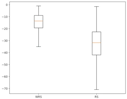
We compare our results against RS, on the same search space, performing 1000 trials on 10000 runs. Table 2 shows the best result achieved by both RS and WRS across all 10000 runs, as well as the average value and the standard deviation of the achieved results across all runs. The standard error for the t-test is 0.176,df = 19998 and P-value≤0.001.
Table 2: WRS vs. RS results for G∗6 - values for 1000 runs
Optimizer Best Found Value Average Value SD
RS -1.50 -33.10 14.06
WRS -1.28 -14.58 10.63
The results obtained by WRS are clearly better than the ones achieved by RS, as also depicted in Fig. 1.
Fig. 2 shows the results obtained for one optimization session with 1000 trials. It can be observed that the algorithm tends to achieve improving results as the number of trials increases.
Figure 1: Performance of WRS vs. RS for theG∗6 optimization
Figure 2: Convergence of WRS for theG∗6 function
5
CNN hyperparameter optimization
Our next application of the WRS is for the optimization of a CNN architecture. Currently CNN in one of the best and most used tools for image recognition and machine vision [25] and there has been a lot if interest in developing optimal CNN architectures [13, 19, 31, 33]. Current CNN architectures are complex, with a high number of hyperparameters. In addition, the training sets for CNNs are large and this increases training times. Hence, we have a high number of trials, each trail with significant execution time. Decreasing the number of trials is critical.
When applying WRS to our CNN optimization problem we consider the following hyperpa-rameters:
• The number of convolution layers - an integer value in the set{3,4,5,6};
• The number of fully-connected layers - an integer value in the set{1,2,3,4};
• The number of output filters in each convolution layer - an integer value in the range
[100,1024];
• The number of neurons in each fully connected layer - an integer value in the range
[1024,2048].
We generate each hyperparameter according to the uniform distribution and assess the performance of the model solely by the classification accuracy.
We use Keras [6] to train and test the CNN for 300 trials - ten epochs each - on the CIFAR-10 [37] dataset. We run our test on an IBM S822LC cluster with IBM POWER8 nodes, NVLink
and NVidia Tesla P100 GPUs2. The CIFAR-10 dataset consists of 6000032×32 color images
in 10 classes, with 6000 images per class. The data is split into 50000 training images and 10000 test images. We do not use data augmentation.
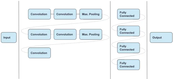
The base architecture of the network is represented in Fig. 3. The model has between
three and six 3×3convolutional layers and between one and four fully connected layers. Both
the convolutional and fully connected layers use ReLU [23] activation and the output layer
uses softmax. We add one 2×2 MAX pooling layer with a dropout [25] of 0.25 for every
two convolutional layers and use a dropout of 0.5 for the fully connected layers. We compare the results obtained by our WRS algorithm against the ones obtained by the RS, Nelder-Mead (NM), Particle Swarm (PS) [16] and Sobol Sequences (SS) [30] implementations provided by Optunity [39].
,QSXW
&RQYROXWLRQ &RQYROXWLRQ 0D[3RROLQJ
&RQYROXWLRQ &RQYROXWLRQ 0D[3RROLQJ
&RQYROXWLRQ )XOO\ &RQQHFWHG )XOO\ &RQQHFWHG )XOO\ &RQQHFWHG )XOO\ &RQQHFWHG 2XWSXW &RQYROXWLRQ 0D[3RROLQJ &RQYROXWLRQ 0D[3RROLQJ )XOO\ )XOO\ )XOO\
Figure 3: The CNN architecture
After the first phase of the algorithm, which consists in running RS for300/e= 110 trials,
we obtain the weights for each parameter. These values, along with the probabilities of change, are listed in Table 3. After running fANOVA, the resulted most important three parameters are (in decreasing order of their weights): the number of neurons in the first fully connected layer,
the number of fully connected layers, and the number of convolutional layers. The weights of the other parameters are more than an order of magnitude smaller. Therefore, the second phase of WRS clearly favors the change in the first three most important parameters.
Table 3: Parameter weights and probabilities for CNN Convolutional Fully Connected
Layers Layers Conv 1 Conv 2 Conv 3 Conv 4 Conv 5 Conv 6 Full 1 Full 2 Full 3 Full 4
7.4 11.85 0.51 0.79 1.62 0.73 2.26 1.26 26.28 0.87 3.22 1.75
0.28 0.45 0.02 0.03 0.06 0.03 0.09 0.05 1.00 0.03 0.12 0.07
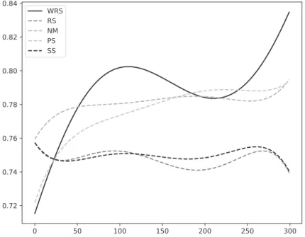
Fig. 4 shows the least squares five degree polynomial fit on the accuracy results obtained for each of the 300 trials using: WRS - the solid line, RS, NM, PS, SS - the dashed lines. The trend of the WRS performance is similar to the one from Fig. 1. The plot considers the actual values, reported at each iteration, instead of the local best in order to better reveal the variation of those values.
Figure 4: Least squares five degree polynomial fit on RS, NM, PS, SS vs. WRS accuracy for CIFAR-10 on 300 trials. The plot considers the values reported at each iteration
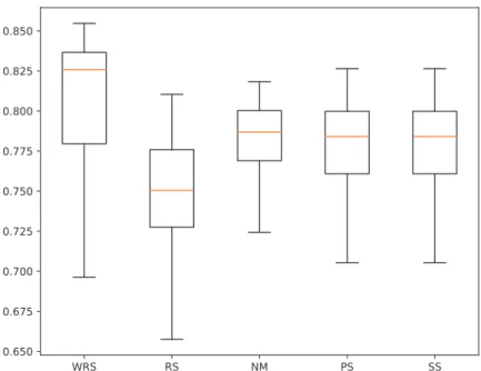
The best accuracy, as well as the average and standard deviation, across all 300 trials for all algorithms, are depicted in Table 4. WRS method outperforms all other considered methods (see Table 4 and Fig. 5).
Table 4: Algorithms’ results for CNN accuracy on CIFAR-10
Optimizer Best Result Average SD
WRS 0.85 0.79 0.09
RS 0.81 0.75 0.04
NM 0.81 0.77 0.03
PS 0.83 0.78 0.03
SS 0.82 0.75 0.05
Figure 5: Performance of WRS, RS, NM, PS and SS for CNN optimization
WRS and RS methods, the resulted architectures have only one fully connected layer and several convolutional layers (five for RS, six for WRS).
Table 5: Best identified CNN architectures on CIFAR-10
Optimizer Convolutional Fully Connected
Layers Layers Conv 1 Conv 2 Conv 3 Conv 4 Conv 5 Conv 6 Full 1 Full 2 Full 3 Full 4
WRS 6 1 736 508 664 916 186 352 1229 - -
-RS 5 1 876 114 892 696 617 - 1828 - -
-NM 5 3 564 564 564 560 563 - 1529 1542 1542
-PS 5 1 479 792 584 411 593 - 1379 - -
-SS 5 2 402 933 750 997 777 - 1545 1268 -
-Table 6: WRS Accuracy Average and Standard Deviation. Row headings are numbers of fully connected layers while column headings are numbers of convolutional layers
FC /C 1 2 3 4 3 0.74 (0.02) 0.70 (0.03) 0.74 (0.01) 0.69 (0.03) 4 0.78 (0.01) 0.74 (0.03) 0.74 (0.03) 0.63 (0.07) 5 0.81 (0.02) 0.80 (0.02) 0.74 (0.07) 0.65 (0.06) 6 0.82 (0.01) 0.76 (0.04) 0.72 (0.09) 0.39 (0.21)
Table 6 details the results obtained by WRS, showing the accuracy average and the standard deviation values for each combination: (number of fully connected layers, number of convolutional layers). Table 7 shows the number of trials performed by WRS for each of these combinations.
We notice that the WRS algorithm favors one of the combinations, namely {1, 6}, and uses it for almost two thirds of the number of trials. It is important to mention that within the best 200 trials, only 10 sets of values contain a different combination than {1, 6}. This is either {1, 5} - seven times, or {2, 5} - three times. The first different combination than {1, 6} is at the 136-th position. In Table 6, we observe that this combination also triggers the best results.
Table 7: WRS Number of Trials. Row headings are numbers of fully connected layers while column headings are numbers of convolutional layers
FC /C 1 2 3 4 3 4 4 4 7 4 8 3 8 9 5 9 7 9 4 6 199 6 10 9
hypothesis that the probability that this combination of hyperparameters corresponds to the global optimum is higher than for any other combination.
6
Conclusions
We have introduced an improved version of RS, the WRS method. Within the same com-putational budget (i.e., for the same number of iterations), WRS converges on average faster than RS. The WRS algorithm yields better results both for the optimization of a well known difficult mathematical function and for a CNN hyperparameter optimization problem. There is little information required to be transferred between the consecutive steps of the algorithm, as pointed out in the description of Algorithm 1. This implies that the WRS algorithm can be easily implemented in parallel. Since we made no assumptions on the objective function, our results can be generalized to other optimization problems defined on a discrete domain. We plan to test out algorithm on other classes of optimization problems, in particular on the optimization of various machine learning algorithms. We also plan to compare the results obtained with WRS with other more complicated optimization techniques, especially from the very promising area of Bayesian optimization.
Author contributions. Conflict of interest
The authors contributed equally to this work. The authors declare no conflict of interest.
Bibliography
[1] Albelwi, S.; Mahmood, A. (2017). A framework for designing the architectures of deep
convolutional neural networks. Entropy, 19, 6 (2017).
[2] Bergstra, J.; Bardenet, R.; Bengio, Y.; Kegl, B. (2011). Algorithms for hyper-parameter
optimization. InNIPS (2011), J. Shawe-Taylor, R. S. Zemel, P. L. Bartlett, F. C. N. Pereira,
and K. Q. Weinberger, Eds., 2546–2554, 2011.
[3] Bergstra, J.; and Bengio, Y. (2012). Random Search for Hyper-Parameter Optimization.
Journal of Machine Learning Research, 13, 281–305, 2012.
[4] Bergstra, J.; Komer, B.; Eliasmith, C.; Yamins, D.; and Cox, D. D. (2015). Hyperopt: a
Python library for model selection and hyperparameter optimization.Computational Science
[5] Chang, C.-C.; Lin, C.-J. (2011). LIBSVM: A library for support vector machines, ACM Transactions on Intelligent Systems and Technology 2, 2(3), 27:1–27:27, 2011. Software
available at http://www.csie.ntu.edu.tw/~cjlin/libsvm.
[6] Chollet, F., et al. (2015). Keras. https://keras.io, 2015.
[7] Claesen, M.; Simm, J.; Popovic, D.; Moreau, Y.; Moor, B. D. (2014). Easy Hyperparameter
Search Using Optunity, CoRR abs/1412.1114, 2014.
[8] Domhan, T.; Springenberg, J. T.; Hutter, F. (2015). Speeding up automatic hyperparameter
optimization of deep neural networks by extrapolation of learning curves, InProceedings of
the 24th International Conference on Artificial Intelligence, IJCAI’15, AAAI Press, 3460–
3468, 2015.
[9] Florea, A. C.; Andonie, R. (2018). A Dynamic Early Stopping Criterion for Random Search
in SVM Hyperparameter Optimization, In 14th IFIP International Conference on Artificial
Intelligence Applications and Innovations (AIAI) (Rhodes, Greece, May 2018), L. Iliadis,
I. Maglogiannis, and V. Plagianakos, Eds., vol. AICT-519 of Artificial Intelligence
Applica-tions and InnovaApplica-tions, Springer International Publishing, Part 3: Support Vector Machines,
168–180, 2018.
[10] Griewank, A. (1981). Generalized decent for global optimization, Journal of Optimization
Theory and Applications, 34, 11–39, 1981.
[11] Hall, M.; Frank, E.; Holmes, G.; Pfahringer, B.; Reutemann, P.; Witten, I. H. (2009). The
WEKA data mining software: An update, SIGKDD Explor. Newsl., 11(1), 10–18, 2009.
[12] Hansen, N.; Müller, S. D.; Koumoutsakos, P. (2003). Reducing the time complexity of
the derandomized evolution strategy with covariance matrix adaptation (cma-es), Evol.
Comput., 11(1), 1–18, 2003.
[13] He, K.; Zhang, X.; Ren, S.; Sun, J. (2016). Deep residual learning for image recognition,
2016 IEEE Conference on Computer Vision and Pattern Recognition (CVPR), 770–778,
2016.
[14] Hinton, G. E. (2012). A practical guide to training Restricted Boltzmann Machines, In
Neural Networks: Tricks of the Trade (2nd ed.), G. Montavon, G. B. Orr, and K.-R. MĂźller,
Eds., vol. 7700 of Lecture Notes in Computer Science. Springer, 599–619, 2012.
[15] Hutter, F.; Hoos, H.; Leyton-Brown, K. (2014). An efficient approach for assessing
hyperpa-rameter importance, In Proceedings of International Conference on Machine Learning 2014
(ICML 2014), 754-762, 2014.
[16] Kennedy, J.; Eberhart, R. C. (1995). Particle swarm optimization, In Proceedings of the
IEEE International Conference on Neural Networks, 1942–1948, 1995.
[17] Kirkpatrick, S. (1984). Optimization by simulated annealing: Quantitative studies,Journal
of Statistical Physics, 34(5), 975–986, 1984.
[18] Kotthoff, L.; Thornton, C.; Hoos, H. H.; Hutter, F.; Leyton-Brown, K. (2017). Auto-WEKA
2.0: Automatic model selection and hyperparameter optimization in WEKA. Journal of
[19] Krizhevsky, A.; Sutskever, I.; Hinton, G. E. (2012). Imagenet classification with deep
con-volutional neural networks, In Proceedings of the 25th International Conference on Neural
Information Processing Systems - Volume 1 (USA, 2012), NIPS’12, Curran Associates Inc.,
1097–1105, 2012.
[20] LeCun, Y.; Bottou, L.; Orr, G.; MĂźller, K. (2012).Efficient Backprop, vol. 7700 LECTURE
NO of Lecture Notes in Computer Science (including subseries Lecture Notes in Artificial
Intelligence and Lecture Notes in Bioinformatics). Springer, 9–48, 2012.
[21] Lemley, J.: Jagodzinski, F.; Andonie, R. (2016). Big holes in big data: A Monte Carlo
algorithm for detecting large hyper-rectangles in high dimensional data, In 2016 IEEE 40th
Annual Computer Software and Applications Conference (COMPSAC), 1, 563–571, 2016.
[22] Li, L.; Jamieson, K. G.; DeSalvo, G.; Rostamizadeh, A.; Talwalkar, A. (2016). Efficient
hyperparameter optimization and infinitely many armed bandits. CoRR abs/1603.06560,
2016.
[23] Nair, V.; Hinton, G. E. (2010). Rectified linear units improve restricted boltzmann machines, InProceedings of the 27th International Conference on International Conference on Machine Learning (USA, 2010), ICML’10, Omnipress, 807–814, 2010.
[24] Nelder, J. A.; Mead, R. (1965). A Simplex Method for Function Minimization, Computer
Journal, 7, 308–313, 1965.
[25] Patterson, J.; Gibson, A. (2017).Deep Learning: A Practitioner’s Approach, 1st ed. O’Reilly
Media, Inc., 2017.
[26] Pedregosa, F.; Varoquaux, G.; Gramfort, A.; Michel, V.; Thirion, B.; Grisel, O.; Blondel, M.; Prettenhofer, P.; Weiss, R.; Dubourg, V.; Vanderplas, J.; Passos, A.; Cournapeau, D.; Brucher, M.; Perrot, M.; Duchesnay, E. (2011). Scikit-learn: Machine learning in Python,
Journal of Machine Learning Research, 12, 2825–2830, 2011.
[27] Shahriari, B.; Swersky, K.; Wang, Z.; Adams, R. P.; de Freitas, N. (2016). Taking the human
out of the loop: A review of bayesian optimization. Proceedings of the IEEE, 104, 148–175,
2016.
[28] Smusz, S.; Czarnecki, W. M.; Warszycki, D.; Bojarski, A. J. (2015). Exploiting uncertainty
measures in compounds activity prediction using support vector machines, Bioorganic &
medicinal chemistry letters, 25(1), 100–105, 2015.
[29] Snoek, J.; Larochelle, H.; Adams, R. P. (2012). Practical bayesian optimization of machine
learning algorithms, In Advances in Neural Information Processing Systems 25, F. Pereira,
C. J. C. Burges, L. Bottou, and K. Q. Weinberger, Eds. Curran Associates, Inc., 2951–2959, 2012.
[30] Sobol, I. (1976). Uniformly distributed sequences with an additional uniform property,USSR
Computational Mathematics and Mathematical Physics, 16(5), 236 – 242, 1976.
[31] Szegedy, C.; Liu, W.; Jia, Y.; Sermanet, P.; Reed, S.; Anguelov, D.; Erhan, D.; Vanhoucke,
V.; Rabinovich, A. (2015). Going deeper with convolutions, InComputer Vision and Pattern
[32] Thornton, C.; Hutter, F.; Hoos, H. H.; Leyton-Brown, K. (2013). Auto-WEKA: Combined
selection and hyperparameter optimization of classification algorithms, InProceedings of the
19th ACM SIGKDD International Conference on Knowledge Discovery and Data Mining
(New York, NY, USA, 2013), KDD ’13, ACM, 847–855, 2013.
[33] Zeiler, M. D.; Fergus, R. (2014). Visualizing and understanding convolutional networks. In Computer Vision – ECCV 2014 (Cham, 2014), D. Fleet, T. Pajdla, B. Schiele, and
T. Tuytelaars, Eds., Springer International Publishing, 818–833, 2014.
[34] Zoph, B.; Le, Q. V. (2016). Neural architecture search with reinforcement learning, CoRR
abs/1611.01578 (2016).
[35] Zoph, B.; Vasudevan, V.; Shlens, J.; Le, Q. V. (2017). Learning transferable architectures
for scalable image recognition. CoRR abs/1707.07012, 2017.
[36] [Online]. Bigml; BigML, Inc.https://bigml.com/ Accessed: 2019-01-10.
[37] [Online]. Cifar 10; Krizhevsky, A., Nair, V., and Hinton, G.https://www.cs.toronto.edu/
~kriz/cifar.html Accessed: 2019-01-10.
[38] [Online]. Google HyperTune, Google. https://cloud.google.com/ml-engine/docs/
tensorflow/using-hyperparameter-tuning Accessed: 2019-01-10.
[39] [Online]. Optunity,http://optunity.readthedocs.io/en/latest/. Accessed: 2019-01-10.