San Jose State University
SJSU ScholarWorks
Master's Projects Master's Theses and Graduate Research
Spring 5-22-2019
Deep Learning on Graphs using Graph
Convolutional Networks
Saurabh Mithe
San Jose State UniversityFollow this and additional works at:https://scholarworks.sjsu.edu/etd_projects
Part of theArtificial Intelligence and Robotics Commons, and theTheory and Algorithms Commons
This Master's Project is brought to you for free and open access by the Master's Theses and Graduate Research at SJSU ScholarWorks. It has been accepted for inclusion in Master's Projects by an authorized administrator of SJSU ScholarWorks. For more information, please contact
Recommended Citation
Mithe, Saurabh, "Deep Learning on Graphs using Graph Convolutional Networks" (2019).Master's Projects. 720. DOI: https://doi.org/10.31979/etd.yca4-fmqh
Deep Learning on Graphs using Graph Convolutional Networks
Project Presented to
The Faculty of the Department of Computer Science San Jose State University
In Partial Fulfillment
of the Requirements for the Degree Master of Science
by Saurabh Mithe
c
○2019
Saurabh Mithe ALL RIGHTS RESERVED
The Designated Project Committee Approves the Project Titled
Deep Learning on Graphs using Graph Convolutional Networks
by Saurabh Mithe
APPROVED FOR THE DEPARTMENT OF COMPUTER SCIENCE
SAN JOSE STATE UNIVERSITY
May 2019
Dr. Katerina Potika Department of Computer Science
Dr. Sami Khuri Department of Computer Science
ABSTRACT
Graphs are a powerful way to model network data with the objects as nodes and the relationship between the various objects as links. Such graphs contain a plethora of valuable information about the underlying data which can be extracted, analyzed, and visualized using Machine Learning (ML). The challenge to this task is that graphs are non-Euclidean structures which means that they cannot be directly used with ML techniques because ML techniques only work with Euclidean structures like grids or sequences. In order to overcome this challenge, the graph structure first needs to be encoded into an equivalent Euclidean representation in the form of a low-dimensional vector. This low-dimensional vector is called an embedding vector, and the encoding process is called node embedding. Traditionally, user-defined heuristics and matrix-factorization based methods were used for node embedding. However, these methods are slow and perform poorly on large and complex graphs. During the recent years, various ML techniques have been developed that learn the encoding of the graph automatically, and in a faster and more efficient way. A few of these techniques called Graph Convolutional Networks (GCNs) use variants of the convolutional neural networks adapted for graphs, and are implemented using deep neural networks. The aim of this project is two-fold. Firstly, to develop a unified framework focusing on three major GCN techniques in order to analyze, evaluate, and compare their performance on select benchmark datasets for the task of node classification. And secondly, to implement a new aggregator for one of the techniques — GraphSAGE, and compare the performance of the aggregator with the existing GCN methods as well as the other aggregators provided by GraphSAGE.
Index Terms — Node embedding, machine learning, graph convolutional
ACKNOWLEDGMENTS
I would like to take this opportunity to express my gratitude towards my advisor and mentor - Dr. Katerina Potika. I was fortunate enough to work with her and receive guidance on my master’s project, a decision which I took as a result of taking the courses on social networks, graphs, and algorithm analysis under her guidance and realizing that we share the same interests and passion towards graphs, networks, and the underlying algorithms.
Her knowledge of the field, combined with the relentless enthusiasm and energy towards guiding her students has been evident in every step of the way. She man-aged to keep me motivated to progress in the right direction while making sure I was researching, learning, exploring, and applying the knowledge that would help me successfully complete the project independently while helping me with topics I struggled with. The time, energy, and attention provided by her in this endeavor are truly commendable and I thank her very much for that.
My heartfelt gratitude goes to Dr. Sami Khuri and Dr. Robert Chun for agreeing to be on my defense committee and providing their valuable time, feedback and guidance. Last but not least, I want to thank my colleagues and friends who kept me motivated and supported and helped me through difficult academic challenges.
TABLE OF CONTENTS CHAPTER 1 Introduction . . . 1 1.1 Problem Statement . . . 4 1.2 Terminology . . . 5 1.2.1 Graphs . . . 5 1.2.2 Feature Vectors . . . 7 1.2.3 Neural Networks . . . 9 1.2.4 Node Embeddings . . . 11 1.2.5 Node Classification . . . 13 2 Related Work . . . 15
2.1 Methods using matrix-factorization . . . 15
2.2 Methods using random walk . . . 16
2.3 Methods using auto-encoders . . . 16
2.4 Methods using graph-convolutions . . . 16
2.4.1 Graph Convolutional Networks (GCN) . . . 18
2.4.2 Fast GCN . . . 19
2.4.3 GraphSAGE . . . 20
2.4.4 Graph Attention Networks . . . 22
3 Methodology . . . 23
3.1 Developing a unified analysis framework for evaluating existing methods . . . 25
3.1.2 Fast Graph Convolutional Network (Fast GCN) . . . 27
3.1.3 GraphSAGE . . . 28
3.2 Graph Attention Aggregator Model . . . 29
3.2.1 Principles of attention in graphs . . . 30
3.2.2 Aggregator Model using Attention . . . 31
4 Experiments and Results . . . 33
4.1 Datasets . . . 33
4.1.1 Cora Citation Dataset . . . 33
4.1.2 Pubmed Citation Dataset . . . 34
4.1.3 Citeseer Citation Dataset . . . 35
4.1.4 Reddit Posts Dataset . . . 35
4.2 Generating and visualizing Node Embeddings . . . 36
4.3 Graph Convolutional Networks (GCN) . . . 38
4.3.1 Results . . . 39 4.4 Fast GCN . . . 41 4.4.1 Results . . . 42 4.5 GraphSAGE . . . 44 4.5.1 Results . . . 45 4.6 Attention Aggregator . . . 47 4.6.1 Results . . . 47
4.7 Experimentation: Performance comparison of all the techniques . 50 4.8 Experimentation: Performance comparison of attention aggregator with other techniques . . . 50
LIST OF TABLES
1 Cora Citation Dataset . . . 34
2 Pubmed Citation Dataset . . . 34
3 Citeseer Citation Dataset . . . 35
4 Reddit Posts Dataset . . . 35
5 GCN F1 scores and Accuracy . . . 39
6 Fast GCN F1 scores and Accuracy . . . 42
7 GraphSAGE F1 scores . . . 45
8 Attention Aggregator Supervised F1 scores compared to other ag-gregator score in original papers . . . 47
9 Attention Aggregator Supervised F1 scores compared to other method scores in original paper . . . 48
10 Attention Aggregator Supervised F1 scores compared to other ag-gregator score in experimentation . . . 49
11 Attention Aggregator Supervised F1 scores compared to other method scores in experimentation . . . 50
12 Implementation results for existing methods . . . 50
LIST OF FIGURES
1 A simple graph . . . 5
2 Adjacency matrix representation . . . 6
3 Adjacency list representation . . . 7
4 A simple neural network . . . 10
5 A deep neural network . . . 11
6 Node Embeddings for Zachary Karate Club Graph (DeepWalk [9]) 12 7 Node classification for missing labels (GraphSAGE [12]) . . . 14
8 Input to Graph Convolution-based networks . . . 17
9 Graph Convolutional Network (GCN [4]) . . . 19
10 Neighboring node processing - Fast GCN (left) vs GCN (right) (FastGCN [13]) . . . 20
11 Node aggregation (GraphSAGE [12]) . . . 21
12 Neighborhood aggregation algorithm (GraphSAGE [12]) . . . 21
13 Attention Aggregator Model . . . 32
14 Zachary Karate Club Graph . . . 37
15 Node Embeddings for Zachary Karate Club with Identity Matrix as features . . . 37
16 Node Embeddings for Zachary Karate Club with Shortest Path length as features . . . 38
17 GCN Micro F1 Scores . . . 40
18 GCN Accuracy . . . 40
20 FastGCN Micro F1 Scores . . . 43
21 FastGCN Embeddings Visualization for Cora dataset . . . 44
22 GraphSAGE GCN Aggregator F1 Scores . . . 46
CHAPTER 1 Introduction
A graph is a powerful data model when it comes to modeling data. Any form of network data can be modeled as a graph, with the nodes representing the objects and the links representing the connection between those objects. The major graph-models that dominate the world wide web are social networks which have become an integral part of our life and have remarkably changed the way humans interact with each other and the world. Modern social networks contain a plethora of valuable information about their users which can be analyzed in order to extract relevant insights from it [1] which can then be used for applications like recommending new friends to a user [2] or extrapolating missing information for a user profile. In bioinformatics, graphs are used to model protein-protein interaction [3] which can be analyzed in order to predict the protein functions. In research and literature, the publications can be represented in the form of a graph where two publications are joined by an edge if one publication cites the other publication. This graph can be analyzed to find out the similarity and relationship between various publications as well as to classify them into different categories [4]. One major area where graphs are central is the world wide web (www) where the web pages are modeled as nodes and the links connecting those web pages are modeled as edges. Analysis of the structure of the web is the core foundation of the Page Rank [5] algorithm used by search engines to return relevant web pages in response to the given keyword search.
The graph can be analyzed using proper tools for predicting a future link among any two nodes, labeling the unknown nodes, clustering the node data, recommending new links, allocating resources, etc. The quality of results of the above-mentioned
applications depends on the quality and accuracy of the underlying techniques. This analyzing task is called as graph analysis.
Traditional methods for graph analysis have proven to be inefficient for mod-ern social networks because of the network’s vast size and dynamic nature. This raised the need for using modern data analysis techniques based on machine learning in order to achieve an unprecedented performance gain. However, machine learning techniques are designed to work with data defined on Euclidean domains, such as grids (e.g. images) and sequences (e.g. speech, text), and cannot be directly used with data defined on non-Euclidean domains such as graphs [6]. To overcome this limitation, a technique to convert non-Euclidean data into its equivalent Euclidean representation is needed i.e. a way to transform information contained in graphs into an equivalent representation that can be processed by current machine learning mod-els. When transforming the information contained in the graphs into an equivalent Euclidean representation, it is important that the information in the graph should be preserved as much as possible, thus minimizing the translation loss. The transformed representation is called an embedding (dense vector representation) and the process is called node-embedding or feature/representation learning. Once the embeddings are generated, they can be used with the machine learning/deep learning techniques for tasks such as link prediction, community detection, finding influential nodes in a network, and many more. The quality of the generated embeddings determines the accuracy of the result of these tasks.
Existing methods used to generate embeddings can be broadly divided into two main categories - methods that extract heuristic-based features from a graph which are often slow and inefficient when used with modern complex and large graphs and methods that learn the node representations automatically from a given graph in a
faster and more efficient way using machine learning. The machine learning methods are mainly categorized into the following types:
∙ Factorization-based methods (Laplacian Eigenmaps [7], Inner-product [8])
∙ Random walk-based methods (Deep Walk [9], Node2Vec [10])
∙ Autoencoder-based methods (Deep Neural Graph Representations [8],
Struc-tural Deep Neural Embeddings [11])
∙ Graph convolution-based methods (GraphSAGE [12], Graph Convolutional Net-works [4], FastGCN [13], Graph Attention NetNet-works [14])
This project focuses on three recent techniques from the Graph convolution-based methods which are Graph Convolutional Networks (GCN) [4], FastGCN [13], and GraphSAGE [12] all of which, as the name suggests, use a variant of the traditional convolutional networks adapted to graphs in order to learn the graph representa-tion. The methods are based on deep learning and implemented using state-of-the-art frameworks like TensorFlow and PyTorch. The aim of the project is to:
∙ Study the recent (above mentioned) graph convolution-based methods in depth ∙ Develop a unified framework in order to implement, execute, and evaluate the
methods and analyze/compare the performance/results
∙ Develop a custom aggregator model for the GraphSAGE technique and compare its performance with existing methods and other GraphSAGE aggregators on node classification for benchmark datasets.
1.1 Problem Statement
Graph analysis is an important task because of the rising popularity of social networks, and the increase in the amount of data being generated which is modeled in the form of a graph. Graph analysis using machine learning poses some challenges like encoding the graph into a low-dimensional representation in order to extract relevant features that can be fed into the machine learning models for performing tasks such as node classification, label prediction, link recommendation, etc. Various methods for graph analysis via representation learning using deep learning exist that operate on the same underlying principles and offer similar functionality. However, for each technique, the performance is measured on different types and sizes of data and thus, there is no unified framework that gives an accurate comparison of the existing methods on the benchmark datasets. Also, the datasets which are shared by multiple methods differ with respect to the input format and thus, cannot be readily evaluated with other methods. For example, the GCN [4] is tested on Cora, Citeseer, Pubmed, and NELL datasets while FastGCN [13] is tested on Cora, Pubmed, and Reddit leav-ing out the Citeseer dataset. GraphSAGE is tested on Reddit and Protein-protein interaction (PPI) datasets leaving the other ones out. Moreover, GCN does not men-tion the F1 scores of the test experimentamen-tion results while FastGCN leaves out the accuracy. Thus, it is challenging to compare and evaluate the results of these similar methods on the same datasets. Another area of focus is on GraphSAGE, which is a modular representation learning method where the aggregators are modeled in a plug-and-play type of interface. Another technique for graph analysis using deep learning named Graph Attention Networks (GAT) [14] which uses masked self-attention lay-ers that enables specifying different weights to different nodes in a neighborhood in order to achieve a performance gain over the above-mentioned methods which use the
same weights for all the nodes in the neighborhood. The aim is to develop and im-plement a new aggregation model for GraphSAGE based on the concept of attention over the features of the model as described in the GAT technique instead of a simple mean aggregation and evaluate/compare the performance and the results of the new aggregator method with other methods.
1.2 Terminology
1.2.1 Graphs
A graph is a collection of vertices connected with each other by edges. Graph
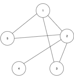
𝐺 can be represented as 𝐺 = (𝑉, 𝐸) where 𝑉 is a set of vertices and 𝐸 is a set of edges where each edge joins two vertices. Figure 1 shows a graph with5 vertices and
6 edges could be represented as follows:
𝑉 ={1,2,3,4,5}
E = {(1,2),(1,3),(2,4),(2,5),(3,2),(5,1)} 𝐺= (𝑉, 𝐸)
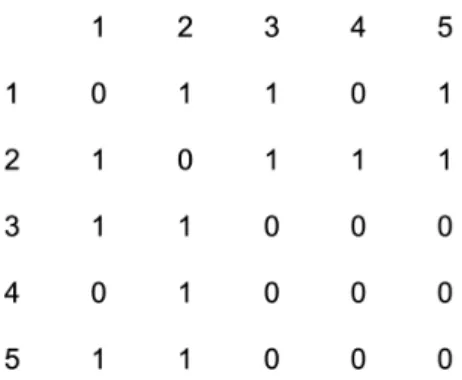
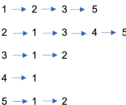
Graphs are abstract data structures i.e they can be implemented and represented in more than one way. A graph representation can be as simple as a list of all edges present in the graph, an adjacency matrix which is a 𝑛 x 𝑛 matrix where n is the number of vertices in the graph representing the presence of an edge as 1 and the absence as 0 for each pair of vertices, or it can be represented in the form of an adjacency list which is a list of all the vertices where each vertex points to a list of its connected vertices. Figure 2 shows the adjacency matrix representation of a simple undirected graph with 5 nodes and 6 edges while Figure 3 shows the adjacency list representation of the same graph.
Edge List:
𝐺= [(1,2),(1,3),(2,4),(2,5),(3,2),(5,1)]
Figure 2: Adjacency matrix representation
Figure 5 represents a deep neural network with multiple hidden layers producing a multi-category output.
Figure 3: Adjacency list representation
1.2.2 Feature Vectors
A vector, in its simplest form, is a series of numbers. It’s similar to a matrix but restricted to a single row and multiple columns. For example, [1,2,6,4,7,0,1] is a vector of size 7.
A feature vector is just a vector consisting of features of a particular object. For example, if we have a cube 𝐶 with width 𝑤, height ℎ, and depth𝑑, then the feature vector for cube 𝐶 can be represented as 𝐶 = [𝑤, ℎ, 𝑑]. For a cube 𝐶1 with width 5, height 7, and depth 3, the feature vector would be 𝐶1 = [5,7,3].
A graph consists of vertices and edges. A graph representing a social network like Facebook will have the vertices as the profiles of individuals and the edges as the "friendship" relation that join two individuals together. In such a graph, the vertices are objects which contain the entire information about the individuals like their name, profile picture, city, country, school information, occupation, the content they like, the comments, the uploaded media, and much more. All this information belonging to a vertex in a graph can be seen as a feature of that vertex i.e. the details of the individual represented by that particular vertex. Such information would be
best represented using a feature vector. For example, a person John Doe having a Facebook account would have information such as name, city, university, and country. This information can be represented for John as ["John Doe", "Seattle", "University of Washington", "United States of America"]. Other individuals in the graph can be represented similarly. This way of representing objects using in the form of a feature vector allows you to define a common format of information representation allowing only the desired information leaving any unnecessary details out. These feature vectors can then be used in some form of application or information processing system for analysis and information extraction.
The contents of the feature vector for an object is highly dependent on the type of data present in the object as well as the task for which the vector is eventually going to be used. For example, a graph consisting of research papers as vertices with the edges representing the citation of papers by each other could have a feature vector consisting of the top 100 most frequently occurring words present in each of those papers. For example, consider the following papers represented by their feature vectors ignoring the commonly occurring words in the English language:
Paper A: ["denmark", "biology", "molecules", "synthesis", "analysis"] Paper B: ["oxygen", "molecules", "global warming", "ozone", "methane"] Paper C: ["greenhouse", "molecules", "analysis", "ozone", "carbon monoxide"]
The above three papers selected from a group of papers written about global warming could have the respective set of most frequently occurring words extracted using the "TF-IDF" algorithm. These vectors give us a high-level idea about the contents of the papers and eliminate unnecessary information like the commonly occurring or less frequently occurring words, punctuation symbols, special characters, images, etc. Looking at the feature vectors allows us to determine that these papers
belong to a similar topic even if we did not know originally that they are from "global warming" category. Thus, feature vectors are a powerful way of representing and leveraging the information present in a graph.
In cases where the graph objects do not have any explicit features, the structural properties of the vertices such as in-degree, out-degree, page rank, centrality, etc. can be used to represent the properties of the objects in order to be used in the analysis of the graph.
1.2.3 Neural Networks
Neural Networks are a set of algorithms modeled after the human brain designed to recognize patterns in the input data based on some set of rules. These networks are capable of remembering the previously seen information and associating it with the new information in order to selectively learn and remember the required information. In the end, the learned patterns are stored as a "model" which can then be used to make informed decisions on the new or previously unseen data.
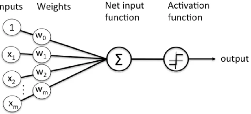
The way in which neural networks operate is that they use a structural unit called as a node which is analogous to a neuron present in the human brain. A neural network can contain hundreds or even thousands of such neurons or nodes. A node gets activated only if the input that the particular node receives meets certain criteria defined by an "activation function". Different nodes receive different information from the same input based on the way the network is designed. The nodes are connected with each other using "weights" which are a set of floating point numeric values that get updated upon each activation. Eventually, the set of the values represented as weights are fine-tuned based on input and these values can be used to make a prediction on the new input data. This is what we call as "learning" in terms of
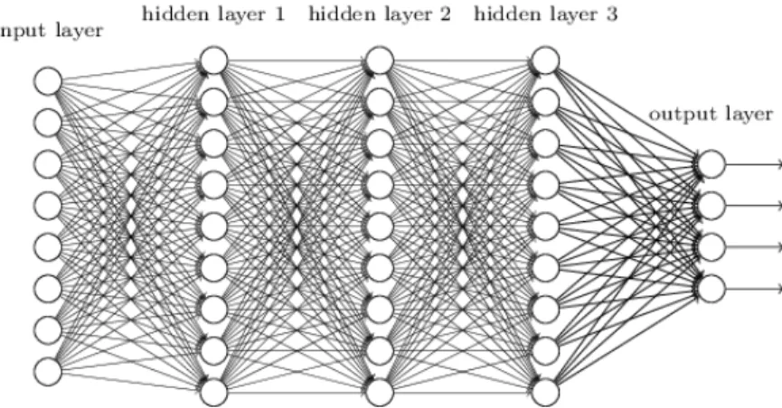
"machine learning" which makes neural networks a specific form of machine learning. While it is totally normal for a neural network to have a single "layer" of such nodes, adding more layers increases the performance of the neural network dramat-ically. Each of these layers can be stacked together in order to form a much more complex and capable neural network which is called as a "deep neural network" with the word "deep" insisting on the presence of multiple layers called as "hidden layers". The learning done using a deep neural network is thereby called "deep learning". Figure 4 represents a single-layer perceptron model of a neural network with a set of inputs being passed through an input function and an activation layer in order to create an output.
Figure 5: A deep neural network
The above network represents just one type of neural network - a multi-layer perceptron. These types of networks are particularly useful in learning numeric or text data but do not generally perform well on images or sequences like speech and long texts. There are other neural networks which are more suited for images called as "Convolutional neural networks" and those which are suited for long sequences such as "Long short term memory networks" or LSTMs or "Recurrent neural net-works" or RNNs. There is no one right answer when it comes to neural networks as they are highly dynamic and can be modeled based on a particular use case. It is not uncommon to see several different variants of neural networks of each of the above-mentioned types in order to address different kinds of problems across multiple domains.
1.2.4 Node Embeddings
Given a graph containing 𝑛 nodes and 𝑒 edges, an equivalent representation with dimension 𝑑 << 𝑛 is expected as an output of the node embedding process. In some cases like graph convolutional networks, the node embedding process could be combined with the eventual machine learning task such as node classification,
etc. to create a single homogeneous program that accepts the graph as an input and provides the classification result for each node while generating and using the embeddings intermediately.
Also, not all embeddings are created equal. Based on the type of application the generated embedding is going to be used for, the nature of embedding is decided. For example, the embeddings that need to be generated for the task of link prediction would be different from the ones generated for the task of finding influential nodes in a network. This can be done in a supervised manner where the target application would define the process of node embedding itself. Although a generalized embedding would get the work done for all the applications, it wouldn’t be as much effective as a custom embedding generated for that particular application. This is an area that needs to be researched in more detail. Figure 6 represents the node embeddings generated for Zachary Karate Club graph where the nodes belonging to the same group in the original graph are close to one another in the corresponding embedding space.
Figure 6: Node Embeddings for Zachary Karate Club Graph (DeepWalk [9])
Another aspect of node embeddings is based on how the process works for dy-namic graphs where new nodes are being added continuously for example in a social
network where hundreds of new users sign up in a day. The embedding generation technique should also take into consideration the dynamic nature of the graphs and how that can be addressed using the minimum number of computational steps.
1.2.5 Node Classification
Node classification is a classic graph-based problem. Given a graph with several nodes, a set of links connecting those nodes, and a set of categories that the nodes belong to, the idea is to classify the nodes to their respective categories based on some information extraction and analysis based algorithm. For example, given a set of research papers where each paper belongs to exactly one of the seven given categories, the aim is to classify each paper to the respective category that it belongs to. The classification may depend on the text present inside each of the research papers or the topic of the paper, or even the authors of the paper.
Node classification problem may or may not have pre-defined categories. In case we do not know the categories in advance, it is up to us to determine the number of categories and thelabel of each category. For example, node classification can be im-portant in community detection problem in which, given a set of nodes representing people in a city in the form of a graph, we need to determine the different commu-nities the people belong to. Once again, the details of the community determination would be guided by the exact problem we are trying to solve the overall idea remains common. The number of communities can be determined based on the graph size, nature of the data, or some other parameter. Figure 7 represents the scenario where the original graph has a few nodes missing the labels which can be predicted using the machine learning algorithm.
Figure 7: Node classification for missing labels (GraphSAGE [12])
Another area where node classification can prove to be immensely helpful is in the cases where the information about some nodes is not present. In such cases, the nodes can be classified based on the information present in the other nodes and then, once we have categories of the nodes, the information or the labels of the "known" nodes can be propagated over to the unknown nodes in the same category since we know that the nodes belonging to the same category share the similarities.
CHAPTER 2 Related Work
The suggested work in the project conceptually builds upon previous node-embedding techniques that use both supervised and unsupervised form of deep learn-ing on graphs. Traditionally, user-defined heuristics which relied on graph statistics such as node degrees or clustering coefficients, kernel functions, or hand-engineered features to measure neighborhood structures were used to extract features to encode information about a graph. These techniques used graph kernels and treated feature extraction as a pre-processing step performed before the task of classifying the nodes and other similar operations. While the techniques were more efficient than the older methods, they were not fast enough for larger graphs that have over a million or more nodes. To overcome this shortcoming of traditional techniques, newer techniques were developed which use ML and dimensionality reduction principles for the task of fea-ture extraction. The ML techniques automatically learn to encode graph strucfea-ture into an𝑛-dimensional vector using deep learning methods and non-linear dimension-ality reduction principles. They treat the node encoding task like an ML task as compared to treating it like a pre-processing step as done by the older techniques mentioned above. The ML techniques include the following methods:
2.1 Methods using matrix-factorization
These methods are inspired by classic techniques that rely on the concept of
dimensionality-reduction and multi-dimensional scaling. Two major methods are
Laplacian eigenmaps [7] and Inner product methods such as Graph Factorization and GraRep [8].
2.2 Methods using random walk
These methods learn the features by performing random walks on different parts of the graph and then using the collected data to generate embeddings. The intuition behind these approaches is that similar nodes tend to occur together and frequently on random walks started from different nodes. There are two main random walk-based techniques — Node2Vec [10] and DeepWalk [9].
2.3 Methods using auto-encoders
These approaches use auto-encoders to compress the information from a node’s neighbors such that a node’s reaching distance is calculated with respect to all the other nodes and stored in a high-dimensional vector. The dimensionality of this vector is reduced by passing it through an auto-encoder resulting in a much smaller embed-ding representation which can be decoded to retrieve the original embedembed-dings. The two main techniques based on this approach are Deep Neural Graph Representations (DNGR) [8] and Structural Deep Neural Embeddings (SDNE) [11].
2.4 Methods using graph-convolutions
Graph convolution-based approaches are based on the principle of aggregating information from a node’s local neighborhood in order to generate an embedding for it. The advantage of graph convolution-based approaches is that they utilize node features or attributes in order to generate embeddings. In a social network, the node attributes might be the user information such as place of residence, school, workplace, etc. which can be used to further refine the embeddings. In networks where the node attributes are not present, graph statistics like node degree or position can be used as a node attribute.
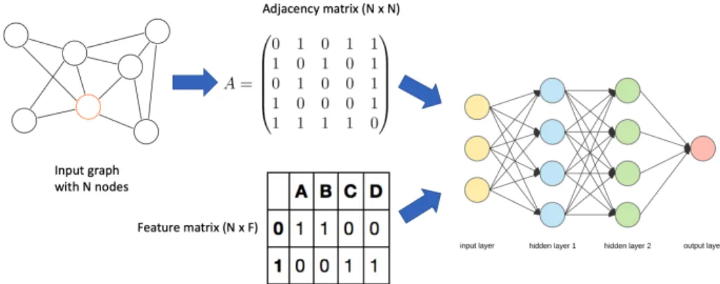
These approaches generate embeddings in a recursive manner. The initial node embeddings are the same as the features of the graph. At each iteration of the algorithm, information is collected from the node’s neighbors and combined with the node’s own feature vector representation. This continues for 𝑘 iterations and in each iteration, more an more information gets carried over to a node (information from𝑘th degree connected node). After the aggregation and combination phases are complete with 𝑘-iterations, the node has information about farther nodes but with the same dimensionality that it started with, which makes it more efficient as compared to other techniques. Figure 8 represents a graph convolutional network where the inputs are in the form of an Adjacency Matrix representation𝐴of the graph along with an input Feature Matrix 𝑋.
Figure 8: Input to Graph Convolution-based networks
A few of the popular recent techniques that are based on the above mentioned principle are GraphSAGE [12], GCN [4], and FastGCN [13] which follow similar underlying principles but differ in implementation. In all the methods, the node embeddings are initialized to be the same as input node attributes. These attributes can be represented using one-hot encoding. In each iteration, the nodes update their own features by aggregating the features of their neighbors using an aggregation
function. After a specific number of iterations, each node has a feature vector that contains information aggregated from its neighbors combined with its own features. This is similar to how a convolution operator would operate on images or grids in order to aggregate information about the image by looking at the surrounding pixel information.
2.4.1 Graph Convolutional Networks (GCN)
GCN is a technique that uses a semi-supervised method of training. GCN is built on the concept of convolutions which are popular for image identification and processing tasks. In GCN, the information from the adjacent nodes is gathered via a form of localized first-order approximations of spectral convolutions. GCN also takes into account, the node features in the form of a 𝑁x𝐹0 feature matrix 𝑋 where 𝑁 is the number of total nodes and𝐹0 is the number of input features per node. Another input parameter is the adjacency matrix 𝐴 which is a 𝑁x𝑁 matrix. The network consists of multiple hidden layers 𝐻 and at each layer, the features are aggregated to form the next layer’s features using a propagation rule 𝑓. This process, however, is transductive which means that if new nodes are added to the graph, the entire training needs to be repeated for all the nodes, and the learned embeddings cannot be generalized to previously unseen nodes or similar graphs. Figure 9 represents the block diagram of the graph convolutional network working on a publication dataset belonging to 7 different categories with an embedding output accurately showing the separation of the publications into the corresponding categories.
Figure 9: Graph Convolutional Network (GCN [4])
2.4.2 Fast GCN
Fast GCN can be seen as an improvement over the GCN technique proposed by Kipf et. al. While GCN was designed assuming that both training and test data is present while learning features, Fast GCN suggests changes that overcome that requirement. Moreover, in case of large and dense graphs, the way GCN is designed, the recursive neighborhood expansion may result in longer processing times and huge memory consumption, thereby making it difficult or even impossible to use the meth-ods on such types of graphs. Fast GCN provides a solution to this shortcoming by interpreting graph convolutions as integral transforms of the embedding functions under probability measures. Additionally, Fast GCN uses sampling to determine the adjacent nodes that need to be processed instead of processing all the adjacent nodes in case of GCN which improves performance on larger and denser graphs. Figure 10 represents the contrast between the number of nodes processed by GCN (right) and the number of nodes processed by FastGCN (left) which clearly shows that FastGCN saves the processing by a large scale.
Figure 10: Neighboring node processing - Fast GCN (left) vs GCN (right) (FastGCN [13])
2.4.3 GraphSAGE
Most approaches require all the nodes in the graph to be present at the time of training the node features, and are thus transductive in nature. Such approaches do not generalize to previously unseen nodes and require additional rounds of training to be able to do that. GraphSAGE, however, isinductive in nature which means that the features or embeddings, once trained, can be used even when new nodes are added, and instead of training all the features all over again, only the features for the new nodes need to be trained. In addition to that, GraphSAGE allows the learned features to be generalized to an entirely new unseen graph which can potentially save a lot of processing time for seeminglysimilar graphs. This is made possible since GraphSAGE learn a function that generates the node features instead of training individual features for each node. So once the function is learned, new features can be generated for newly added nodes or an entirely new set of nodes for a similar graph. This learned function is called a aggregation function which aggregates the features from the surrounding nodes in order to generate features for a particular node. The general aggregation functions that are implemented in GraphSAGE are element-wise mean aggregator
which, as the name suggests, calculates the mean value of the all features of all the adjacent nodes and aggregates them to form the features for a given node, a max-pooling aggregator which selected the maximum of the features for the adjacent nodes, and LSTM aggregator to aggregate neighboring embedding information. The aggregation step is repeated for𝑘 steps in order to aggregate information from farther nodes. Figure 11 represents the aggregation function for GraphSAGE technique while Figure 12 shows the GraphSAGE aggregation and sampling algorithm to aggregate features from the neighboring nodes for𝑘-iterations.
Figure 11: Node aggregation (GraphSAGE [12])
2.4.4 Graph Attention Networks
Graph Attention Networks (GATs) [14] are a type of Graph Convolutional Net-works (GCNs) which use the concept of attention to overcome the limitations of some of the other GCNs. This is done by allowing the nodes to use different weight for each neighbor while combining the neighborhood features.
CHAPTER 3 Methodology
The embedding technique proposed by Kipf et al. [4] named Graph Convo-lutional Networks uses a weighted element-wise mean to aggregate information from the neighboring nodes and a weighted sum is used to combine the aggregated informa-tion with a node’s own embedding while using node features or attributes. However, this approach is transductive i.e. if new nodes are added to the graph, additional rounds of training need to be performed. Also, the generated embeddings cannot be generalized for other similar graphs.
The embedding technique proposed by Chen et. al. [13] named Fast GCN
improves upon GCN by using a sampling function that operates over a probability measure in order to minimize the number of nodes that are processed for each node. This significantly reduces the processing time and is more suitable for larger and denser graphs. However, it does not address the transductive issues present in GCN. The technique proposed by Hamilton et al. [12] named GraphSAGE uses gen-eral aggregation functions such as element-wise mean, a max-pooling neural network, and LSTMs are used to aggregate neighboring node information and a concatena-tion operaconcatena-tion to combine the aggregated informaconcatena-tion with a node’s own embedding. GraphSAGE is inductive which enables the generation of embeddings for previously unseen nodes thereby making it a better choice over the other two methods for larger dynamic graphs.
GraphSAGE introduces a plug-and-play style of aggregation mechanism for node embedding where different kinds of aggregator functions can be used within the same
implementation based on the required functionality. The mean aggregator and the GCN aggregator are the best performers among all the aggregators suggested by GraphSAGE. A recent paper named Graph Attention Networks (GAT) [14] leverages masked self-attentional stacked layers in which nodes are able to attend over the features of their neighbors in order to aggregate the neighbor features and generate node embeddings for the given node. This project aims to build on the principles of Graph Attention Networks in order to design an aggregator function which can be plugged into the GraphSAGE model in order to generate the node embeddings. This would enable the user to leverage existing properties of GraphSAGE while providing potential improvements achieved using attention in graphs. The performance would be compared with the existing techniques mentioned above as well as with other aggregator functions provided by GraphSAGE.
Since each of the above methods uses different datasets for experimentation, in order to compare the results, it is necessary to implement, and execute the methods on a common set of benchmark datasets and analyze the performance. Moreover, each technique uses different measures in order to showcase the results. For example, GCN relies on accuracy for the experimentation while FastGCN relies entirely on F1 scores. Thus, one of the major challenges in completing the project would be to develop a unified framework in order to implement, execute, and test the performance of the above-mentioned techniques on a common set of benchmark datasets.
The proposed implementation plan for the project is as follows:
∙ Implementing standard Graph Convolution Network, Fast GCN, and
Graph-SAGE techniques.
able to run them on the same set of standard benchmark datasets.
∙ Analyzing the performance of each technique and tune the hyper-parameters until the best performance for the technique is achieved in the given computa-tional environment.
∙ Implementing the custom aggregator for GraphSAGE that uses attention over the neighboring nodes.
∙ Comparing the custom aggregator performance on benchmark datasets with
that of existing techniques as well as other aggregator models.
3.1 Developing a unified analysis framework for evaluating existing
meth-ods
Since all the node embedding techniques implementations being studied in this project differ in one or more key aspects, it is crucial to unifying them by adding the missing features to each of the implementations. This would make it possible to evaluate the performance of all the techniques on a common set of benchmark datasets described in the previous section. Following sections describe the work done and changes made to each of the techniques in order to achieve that goal.
3.1.1 Graph Convolutional Network (GCN)
Graph Convolutional Network (GCN) is a scalable semi-supervised approach for graph analysis based on an efficient variant of convolutional neural networks that operate directly on graphs [4]. The algorithm learns hidden layer representations that encode local graph structure and node features in the given graph.
∙ a 𝑉x𝑉 adjacency matrix representation 𝐴 of the graph 𝐺
∙ an input feature vector 𝑋 of dimensions 𝑉 x 𝐹0 where 𝐹0 is the number of input features per node
The hidden layer 𝐻i can be written as 𝑓(𝐻i-1, 𝐴) where 𝐻0 =𝑋 (input feature vector) and𝑓 is the propagation rule (activation function). On each layer, the features are aggregated from the neighboring nodes to form the features for the next layer. This is continued all the way to the last layer which outputs the final set of features for each node. In this way, the features for each node are learned by the model.
This project uses the original implementation provided by the authors from their official Github repository as a starting point and then builds upon them according to the requirements.
3.1.1.1 Modifications
∙ The original implementation only calculated and used accuracy as a part of their experimentation and results. So this project adds the functionality to calculate the precision, recall, and the micro F1 score for the valida-tion sets. This was important since other methods use the micro F1 measure to compare results which the original implementation was lacking.
∙ A module to extract the node embeddings and visualize them after
the model is trained is developed as a part of the projectusing the tSNE
3.1.1.2 Limitations
∙ The original paper does not showcase the micro F1 scores which are crucial since we need to compare the results with those showcased by other papers who use micro F1 scores. So for the sake of comparison, the micro F1 scores in the results section are taken from the Fast GCN paper results section who ran the experiments on original GCN and provided the F1 scores in their own paper. ∙ Because of the processing overhead for large graphs, and GCN’s inability to
process them, the experiments could not be run for Reddit dataset due to its large size.
3.1.2 Fast Graph Convolutional Network (Fast GCN)
In Graph Convolutional Network [13], the neighborhood expands rapidly, and within a few hops (usually 3-4), the entire graph is covered. This repeats for each node, and thus, to process each node, the entire graph needs to be accessed which is expensive in terms of computation. FastGCN addresses this exact issue by sampling the neighborhood up to a fixed number 𝑘 so that a lot of computations are saved. This substantial reduction in the neighborhood gives the same quality of output as a result of a careful selection of samples under a probability measure using a Monte Carlo approximation of the loss function. Apart from this major change, the rest of the functionality remains similar to that of GCN mentioned in the previous section. This sampling approach yields substantially better results over GCN as showcased below.
3.1.2.1 Modifications
∙ A module to extract the node embeddings and visualize them after
the model is trained is developed as a part of the projectusing the tSNE
dimensionality reduction algorithm which is showcased in the results section.
3.1.2.2 Limitations
∙ Citeseer was not included with the implementation provided by the authors. So the dataset was imported in a format that runs with the implementation and trained the model on that dataset.
∙ The Reddit dataset was not provided with the implementation. So this project implements a custom program to convert the Reddit dataset into the format executable by the provided implementation.
∙ The original paper does not showcase the accuracy which we need to compare the results with those showcased by other papers who use accuracy. There-fore, this project adds the functionality to calculate the accuracy from the test predictions and the original labels for the test set.
3.1.3 GraphSAGE
GraphSAGE [12] can be viewed as a stochastic generalization of graph convolu-tions and is useful for large dynamic graphs with rich feature information.
Since the original implementation of GraphSAGE was intended and designed for massive dynamic graphs, it did not perform well on smaller static graphs which may or may not have node features. The overhead of sub-sampling required for larger graphs makes GraphSAGE perform in a negative way on smaller graphs taking more
execution time and resulting in sub-optimal outcomes.
The author provided a light-weight implementation written using PyTorch to address the above issues making it possible for GraphSAGE to run efficiently on smaller static graphs. However, this implementation only contains the GCN aggre-gator and the mean aggreaggre-gator. The results showcased in the following sections are taken from the implementation which provides a better outcome for the dataset under consideration.
3.1.3.1 Modifications
∙ The GraphSAGE implementation provided by the authors did not experiment
on Cora, Pubmed, and Citeseer datasets which are covered by the other tech-niques. Moreover, the input format for the datasets for GraphSAGE differs from the original format of the datasets. A custom converter module is developed as a part of project work that takes the original dataset as the input and generates an equivalent dataset in the format that works with GraphSAGE. This project uses the converter to convert Cora, Pubmed, and Citeseer datasets before using them with GraphSAGE.
3.1.3.2 Limitations
∙ Citeseer dataset was not provided by the authors, and thus, there were no target results to have a comparison with.
3.2 Graph Attention Aggregator Model
The Graph Convolutional Network is structure-dependent which limits the gen-eralizability of the algorithm. This problem is overcome by GraphSAGE which takes
an average of all the adjacent node features. However, the weights being used for all the adjacent neighbors are the same which does not work well since different nodes have different features, and thus, the weights should be modified independently for each neighbor. Using attention in graphs [14], this problem is overcome by assigning weights to the neighbors based on their features and provide a structure-independent normalization. In essence, in the modified aggregator, attention over the features of neighbors is used in place of the mean aggregation of the node features.
3.2.1 Principles of attention in graphs
In Graph Convolutional Network, a convolutional operator calculated a normal-ized sum of the features of the adjacent nodes. This is done using the following formulae based on GAT [14] and explained on DGL website [15] as follows
ℎ(𝑖𝑙+1)=𝜎(︁∑︀ 𝑗∈𝒩(𝑖) 1 𝑐𝑖𝑗𝑊 (𝑙)ℎ(𝑙) 𝑗 )︁ where
∙ 𝒩(𝑖) is the set of one hop neighbors ∙ 𝑐𝑖𝑗 =
√︀
|𝒩(𝑖)|√︀|𝒩(𝑗)| is the normalization constant ∙ 𝜎 is the activation function (ReLU)
∙ 𝑊(𝑙) is the weight-matrix
GraphSAGE follows the same model but with a different normalization constant as
𝑐𝑖𝑗 =|𝒩(𝑖)|
Steps to calculate attention: The Graph Attention Network technique [14]
1. For a given layer, calculate a linear transformation 𝑧 of the features ℎ of the current layer and the weight matrix𝑊
𝑧𝑖(𝑙) =𝑊(𝑙)ℎ(𝑖𝑙)
2. Calculate a pair-wise attention score𝑒for any two-nodes adjacent to each other. This can be done by concatenating the linear transformations 𝑧 for both the nodes and taking a dot product of the concatenation with a weight vector 𝑎. This entire product is passed through a non-linear activation function 𝜎 which is a LeakyReLU.
𝑒(𝑖𝑗𝑙) =LeakyReLU(⃗𝑎(𝑙)𝑇
(𝑧𝑖(𝑙)||𝑧𝑗(𝑙)))
3. The attention score calculated in the previous step is normalized using a soft-max function. 𝛼(𝑖𝑗𝑙) = exp(𝑒 (𝑙) 𝑖𝑗) ∑︀ 𝑘∈𝒩(𝑖)exp(𝑒 (𝑙) 𝑖𝑘)
4. The features for the next layerℎ+ 1are aggregated from the neighboring nodes after being scaled by their attention scores.
ℎ(𝑖𝑙+1) =𝜎(︁∑︀ 𝑗∈𝒩(𝑖)𝛼 (𝑙) 𝑖𝑗 𝑧 (𝑙) 𝑗 )︁
3.2.2 Aggregator Model using Attention
∙ The attention aggregator which is based on the principles of attention in graphs as mentioned in [14] consists of a Sequential model made up of two Linear layers and a simple hyperbolic tangent activation function tanh. This is used to calculate𝑧(𝑖𝑙) from step1
∙ The attention score𝑒(𝑖𝑗𝑙) is calculated by calculating the embeddings of adjacent nodes and talking its dot product with vector 𝑎(𝑙)𝑇. This is done using a fully connected layer implementing a linear model with an activation function of LeakyReLU.
∙ The calculated attention score is then fed through a soft-max layer in order to normalize them.
CHAPTER 4 Experiments and Results
4.1 Datasets
The machine learning task to be focused on in this project isnode classification has a set of nodes and a set of edges connecting the nodes in the form of a graph. The algorithm classifies the nodes into separate categories such that similar nodes belong to the same category. The datasets chosen for this project are some of the most well-known datasets for node classification.
The choice of a dataset is one of the most important aspects of any data analysis project. When it comes to graph data, there are many available choices that can be attributed to the boom of social networks and the rising popularity of graphs in general. Since we are dealing with the node classification problem here, the dataset we choose should have the data that can be classified into a finite number of categories and should have a good probability that the data is almost uniformly distributed i.e. the data should not be biased and inclined towards a particular category. The datasets chosen for this project are as follows:
4.1.1 Cora Citation Dataset
The Cora dataset consists of 2708 scientific publications classified into one of the seven categories. It has 5429 edges where the presence of each edge indicates a "citation" relationship between two given papers 𝐴 and 𝐵 such that paper 𝐴 cites paper 𝐵.
1433is the number of unique words present in all the papers combined. Such a vector is called a dictionary. Each entry in the feature vector is either a 0 or a 1 with 0
representing the absence of that word in a paper and1representing the presence. For example, if paper number 1652 contains a word "neuron" which is the 57th word in the dictionary of 1433 words, then the value at the 1652nd row and the 57th column would be 1.
Nodes Edges Features Classes Type Source
2708 5429 1433 7 Citation linqs.cs.umd.edu
Table 1: Cora Citation Dataset
4.1.2 Pubmed Citation Dataset
The Pubmed Diabetes dataset consists of 19717 scientific publications related to diabetes classified into one of the three categories. It has 44338 edges where the presence of each edge indicates a "citation" relationship between two corresponding publications.
The feature vector for the dataset consists of500 columns and19717rows where
500 is the number of unique words present extracted using TF/IDF algorithm from all the papers combined. The row and column corresponding to the publication/word is set to 1if the word is present in the paper else 0.
Nodes Edges Features Classes Type Source
19717 44338 500 3 Citation linqs-data.soe.ucsc.edu
4.1.3 Citeseer Citation Dataset
The Citeseer Citation dataset consists of 3312 scientific publications classified into one of the six categories. It has 4732 edges where the presence of each edge indicates a "citation" relationship between two corresponding publications.
The feature vector for the dataset consists of3703 columns and3312rows where
3703 is the number of unique words present in all the papers combined. The row/col corresponding to the publication/word is set to 1 if the word is present in the paper else 0.
Nodes Edges Features Classes Type Source
3312 4732 3703 6 Citation linqs.soe.ucsc.edu
Table 3: Citeseer Citation Dataset
4.1.4 Reddit Posts Dataset
The Reddit Posts dataset consists of 232965 posts created by Reddit users on the platform classified into one of the 41 communities or subreddits. It has 5376619
edges.
The feature vector consists of 602 columns and 232965 rows where 602 is the number of unique words present in all the posts combined.
Nodes Edges Features Classes Type Source
232965 5376619 602 41 Social Networks Posts pushshift.io
4.2 Generating and visualizing Node Embeddings
The graph convolutional networks, by design, are so powerful that even a simple feed-forward network with random weight initialization can provide pretty good re-sults since it takes advantage of the structural properties of the graph as well as the features. Here is a demonstration of the concept on a Zachary Karate Club graph provided with the NetworkX library as shown in Figure 14. An identity matrix 𝐼
is added to the adjacency matrix 𝐴 in order to create self-loops so that nodes can aggregate their own features too. The resulting matrix is normalized by multiplying it with an inverse degree matrix 𝐷−1 to minimize the effect of a large variation in degrees for different nodes. With a simple ReLU activation function in a two-layer feed-forward network with randomly initialized weights, the generated embeddings are significantly accurate.
Embeddings generated by considering the node numbers in their one-hot repre-sentations as node features are shown in Figure 15
Embeddings generated by considering the length of the shortest path from a node to each of the two leaders as node features are shown in Figure 16
Both the plots show a clear separation between the members belonging to two different groups each led by one of the two leaders.
Figure 14: Zachary Karate Club Graph
Figure 15: Node Embeddings for Zachary Karate Club with Identity Matrix as fea-tures
Figure 16: Node Embeddings for Zachary Karate Club with Shortest Path length as features
Although this simple setup is powerful, it is not suitable for large and complex graphs. Following sections describe the operations of Graph Convolutional Networks on such graphs.
4.3 Graph Convolutional Networks (GCN)
∙ The model is implemented in Python using TensorFlow deep learning library. ∙ The configuration for the showcased results: 230 Epochs, 16 Hidden layers,
Learning rate of0.01.
∙ The default implementation for GCN is unable to handle the Reddit dataset because of the large size. This is consistent with the original paper [4] which too did not include the Reddit dataset in the results.
F1 scores are not available for the original implementation.
4.3.1 Results
Table 5 compares the F1 and Accuracy values for the implemented GCN algo-rithm with modifications and the values provided in the original paper [4]. On the test machine, the accuracy scores for all the datasets came out to be marginally bet-ter than the original paper and can be inbet-terpreted to accurately mimic the intended behavior of the algorithm as suggested by the paper. The original F1 scores, however, were not mentioned in the original paper, and are borrowed from FastGCN [13] which did not have the scores for Citeseer dataset. The F1 experimentation scores seem to be lower than those mentioned in FastGCN paper but cannot be verified since those are not the official scores provided by GCN. The algorithm took a very long time to process the Reddit dataset because of the large dataset size and the associated processing overhead.
Dataset Measure Results (Experiments) Results (GCN [4]) Results (FastGCN [13])
Cora F1 0.784 NA 0.865 Accuracy 81.7 81.5 NA Pubmed F1 0.788 NA 0.875 Accuracy 79.3 79.0 NA Citeseer F1 0.716 NA NA Accuracy 70.9 70.3 NA Reddit F1 NA NA NA Accuracy NA NA NA
Figure 17: GCN Micro F1 Scores
Figure 19 displays the node-embeddings in a two-dimensional space, separated into different categories for the Cora publications. As seen from the figure, the em-beddings show that the publications are successfully categorized into 7 clusters with each cluster representing a different category. Since the accuracy of GCN is low, there are some false-positives which can be seen in the form of color-overlapping.
Figure 19: GCN Embeddings Visualization for Cora dataset
4.4 Fast GCN
∙ The model is implemented in Python using TensorFlow deep learning library. ∙ The configuration for the showcased results: 200 Epochs, 128 Hidden layers,
Learning rate of0.01.
∙ FastGCN implementation provided by the authors as well as the paper does
not include experiments run on Citeseer database. The experiments, however, consider Citeseer but I do not have the benchmark original Citeseer accuracy or F1 results to compare with.
∙ FastGCN implementation and the paper does not include accuracy calculation for the experiments performed on the datasets so the comparison with my ac-curacy calculation would not be possible and therefore, is not considered.
4.4.1 Results
Table 6 compares the F1 and Accuracy values for the implemented FastGCN algorithm with modification and the values provided in the original paper. On the test machine, the F1 scores appear to be close to the scores provided in the paper which is in alignment with the conclusions in the original paper. The test implementation calculates the accuracy values for the experiments run on the datasets but they cannot be compared with the original paper [13] since they were not provided with the paper.
Dataset Measure Results (Experiments) Results (Original Paper [13])
Cora F1 0.9098 0.850 Test Accuracy 87.4 NA Pubmed F1 0.881 0.880 Test Accuracy 86.90 NA Citeseer F1 0.8346 NA Test Accuracy 78.7 NA Reddit F1 0.9296 0.937 Test Accuracy 92.6 NA
Figure 20: FastGCN Micro F1 Scores
Figure 21 displays the node-embeddings for the Cora dataset using FastGCN. As seen from the figure, the number of false-positives is significantly less than the ones present in the GCN embeddings shown in Figure 19. This is in line with the accuracy scores for both the techniques where the accuracy of FastGCN for all the datasets is significantly greater than the accuracy of GCN for those datasets.
Figure 21: FastGCN Embeddings Visualization for Cora dataset
4.5 GraphSAGE
∙ The results showcased in this section are derived from two separate implemen-tations of the algorithm. GraphSAGE [12] was initially designed to work effi-ciently on larger graphs, and involve a significant amount of pre-processing for each node. This model is implemented in Python using TensorFlow deep learn-ing library. However, the implementation is not suitable for smaller datasets like
Cora dataset because of the unnecessary processing for its size. The authors, for this exact purpose, provided a simpler implementation in Python using the PyTorch deep learning library.
∙ The configuration for the TensorFlow implementation: 150Epochs, 128Hidden layers, Learning rate of 0.01.
∙ The default GCN provides an implementation for Max-Pool aggregator, Mean
imple-mentation, however, provides only the GCN aggregator and the Mean aggrega-tor implementation since those are the highest-performing among all the aggre-gators on an average. For the purpose of experimentation, this project sticks to the GCN aggregator and the Mean aggregator.
4.5.1 Results
Table 7 compares the F1 scores of the test implementation with those provided by the original paper. Since the datasets Cora and Pubmed were not mentioned in the original paper, this project refers to FastGCN paper [13] tests on GraphSAGE for those scores. The results include scores for both the GCN aggregator and the mean aggregator and shows that the test results are close to the original scores for the Reddit dataset. The scores differ for Cora and Pubmed but a conclusion cannot be derived since the scores are not from the original paper but from FastGCN tests on the original paper.
Dataset Aggregator F1 (Expt.) F1 (GraphSAGE [12]) F1 (FastGCN [13])
Cora GCN Aggr [12] 0.868 NA 0.829 Mean Aggr [12] 0.8760 NA 0.822 Pubmed GCN Aggr [12] 0.83 NA 0.849 Mean Aggr [12] 0.874 NA 0.888 Citeseer GCN Aggr [12] 0.69 NA NA Mean Aggr [12] 0.738 NA NA Reddit GCN Aggr [12] 0.9258 0.930 0.923 Mean Aggr [12] 0.9512 0.950 0.946
Figure 22: GraphSAGE GCN Aggregator F1 Scores
4.6 Attention Aggregator
∙ The aggregator is implemented in Python using PyTorch deep learning library.
4.6.1 Results
Table 8 compares the F1 scores of the GCN and Mean aggregators from the original paper to the F1 score of the GraphSAGE attention aggregator designed as a part of this project. As seen in Table 8, the F1 score for the attention aggregator is marginally higher than those for the default aggregators when it comes to smaller datasets like Cora and Pubmed, however, in case of larger Reddit dataset, the attention aggregator F1 score is lower than the one provided in the original paper. The decrease in score for the Reddit dataset might be a consequence of the larger size which is making the attention aggregator not perform up to the mark. This will be clearer in the subsequent tests.
Dataset Aggregator F1 Score (Original Paper)
Cora GCN Aggr[12] 0.829 Mean Aggr[12] 0.822 Attn Aggr 0.8921 Pubmed GCN Aggr[12] 0.849 Mean Aggr[12] 0.888 Attn Aggr 0.8852 Citeseer GCN Aggr[12] NA Mean Aggr[12] NA Attn Aggr 0.763 Reddit GCN Aggr[12] 0.930 Mean Aggr[12] 0.950 Attn Aggr 0.8964
Table 8: Attention Aggregator Supervised F1 scores compared to other aggregator score in original papers
Table 9 compares the F1 scores of the GCN and FastGCN algorithms to the F1 scores of the GraphSAGE implementation with the attention aggregator. The scores from the attention aggregator are slightly higher than the other methods for Cora
and Pubmed datasets but lower than the other methods for the Reddit dataset. This is right in line with the results showcased in Table 8 where the scores are lower for the Reddit dataset. It may be the case that the attention aggregator is experiencing some issues when it comes to larger datasets which results in a lower F1 score for such datasets.
Dataset Aggregator F1 Score (Original Paper)
Cora
GCN [4] 0.865
FastGCN [13] 0.85
GraphSAGE with Attn Aggr 0.8921
Pubmed
GCN [4] 0.875
FastGCN [13] 0.88
GraphSAGE with Attn Aggr 0.8852
Citeseer
GCN [4] NA
FastGCN [13] NA
GraphSAGE with Attn Aggr 0.763
GCN [4] NA
FastGCN [13] 0.937
GraphSAGE with Attn Aggr 0.8964
Table 9: Attention Aggregator Supervised F1 scores compared to other method scores in original paper
Table 10 compares the F1 scores for the GCN aggregator and the Mean aggre-gator from the test implementation with the F1 score for the attention aggreaggre-gator. Following the previous patterns, the F1 score of the attention aggregator is higher than that of the other aggregator for Cora,Pubmed, and Citeseer datasets but lower for the Reddit dataset. This shows that the attention aggregator needs to perform better on larger datasets and can be a topic for further research.
Dataset Aggregator F1 Score (Experimentation) Cora GCN Aggr [12] 0.868 Mean Aggr [12] 0.876 Attn Aggr 0.8921 Pubmed GCN Aggr [12] 0.83 Mean Aggr [12] 0.874 Attn Aggr 0.8852 Citeseer GCN Aggr [12] 0.69 Mean Aggr [12] 0.738 Attn Aggr 0.763 Reddit GCN Aggr [12] 0.9258 Mean Aggr [12] 0.9512 Attn Aggr 0.8964
Table 10: Attention Aggregator Supervised F1 scores compared to other aggregator score in experimentation
Table 11 compares the F1 scores for the GCN and the FastGCN method with the F1 score for the attention aggregator. The F1 scores for the Cora, Pubmed, and theCiteseer dataset are significantly better than those of GCN and marginally better than those of FastGCN. However, for the Reddit dataset, the attention aggregator does not outperform the other ones.
Dataset Aggregator F1 Score (Experimentation) Cora
GCN [4] 0.784
FastGCN [13] 0.9098
GraphSAGE with Attn Aggr 0.8921
Pubmed
GCN [4] 0.788
FastGCN [13] 0.881
GraphSAGE with Attn Aggr 0.8852
Citeseer
GCN [4] 0.716
FastGCN [13] 0.8346
GraphSAGE with Attn Aggr 0.763
GCN [4] NA
FastGCN [13] 0.9296
GraphSAGE with Attn Aggr 0.8964
Table 11: Attention Aggregator Supervised F1 scores compared to other method scores in experimentation
4.7 Experimentation: Performance comparison of all the techniques
Dataset GCN[4] FastGCN[13] GraphSAGE Mean[12]
Cora 0.784 0.9098 0.868
Pubmed 0.788 0.881 0.874
Citeseer 0.716 0.8346 0.738
Reddit NA 0.9296 0.9512
Table 12: Implementation results for existing methods
4.8 Experimentation: Performance comparison of attention aggregator
with other techniques
Dataset GCN[4] FastGCN[13] GraphSAGE Mean[12] Attention Aggr.
Cora 0.865 0.85 0.822 0.8921
Pubmed 0.875 0.88 0.888 0.8852
Citeseer NA NA NA 0.763
Reddit NA 0.937 0.950 0.8964
CHAPTER 5 Conclusion
This project develops a unified framework for three known node embedding tech-niques, namely Graph Convolutional Network (GCN), Fast GCN, GraphSAGE, in order to make it possible to compare them with each other on the same set of bench-mark datasets. We measured the performance with regards to F1 score and accuracy. This was not possible before since different techniques used different datasets in their own custom input format and showcased different performance measures. One part of the project implements and modifies the node-embedding techniques, and streamlines them in order to work with all the different datasets. Therefore, it generates results in all the expected measures. The experimentation data from Table 12 shows that FastGCN performs consistently better on smaller datasets, which can be attributed to the sampling mechanism that it improves over GCN. However, for theReddit dataset, which has a lot of nodes and edges, and is a larger graph, the GraphSAGE algorithm outperforms the other methods. This is right in line with the fact that GraphSAGE was built for larger graphs and achieves the performance improvement by using batch pre-processing of node features.
Another aspect of the project is to design a new aggregator model for the Graph-SAGE algorithm and analyze/compare the performance of the new model with that of other aggregators as well as other models. Table 13 showcases the performance of the new aggregator model, named attention aggregator, and its comparison with other models as well as the best-performing GraphSAGE aggregator, which is the Mean aggregator. From the experimental results, one can see that the aggregator model performs significantly better than other methods for theCora dataset, which has the
smallest size among all the available datasets. OnPubmed dataset, the attention ag-gregator performs almost the same as all the other methods with the difference being negligible. Since other techniques did not use the Citeseer dataset, the performance of attention aggregator cannot be compared with the original one. Lastly, for the
Reddit dataset, the performance of the attention aggregator is not as good as that of the FastGCN and GraphSAGE Mean aggregator, which is the best performing for the dataset. This might be partly because the attention aggregator seems to have some performance issues when it comes to larger datasets. This is something that can be a part of further research studying the effect of increasingly larger graphs on the aggregator performance.
![Figure 6: Node Embeddings for Zachary Karate Club Graph (DeepWalk [9])](https://thumb-us.123doks.com/thumbv2/123dok_us/9982259.2490777/23.918.200.768.694.916/figure-node-embeddings-zachary-karate-club-graph-deepwalk.webp)
![Figure 7: Node classification for missing labels (GraphSAGE [12])](https://thumb-us.123doks.com/thumbv2/123dok_us/9982259.2490777/25.918.222.744.137.331/figure-node-classification-missing-labels-graphsage.webp)
![Figure 9: Graph Convolutional Network (GCN [4])](https://thumb-us.123doks.com/thumbv2/123dok_us/9982259.2490777/30.918.225.752.128.349/figure-graph-convolutional-network-gcn.webp)
![Figure 10: Neighboring node processing - Fast GCN (left) vs GCN (right) (FastGCN [13])](https://thumb-us.123doks.com/thumbv2/123dok_us/9982259.2490777/31.918.231.748.135.357/figure-neighboring-node-processing-fast-gcn-right-fastgcn.webp)
