SUMMARY
In some cases model-based and model-assisted inferences can lead to very different estimators. These two paradigms are not so different if we search for an optimal strategy rather than just an optimal estimator, a strategy being a pair composed of a sampling design and an estimator. We show that, under a linear model, the optimal model-assisted strategy consists of a balanced sampling design with inclusion probabilities that are proportional to the standard deviations of the errors of the model and the Horvitz–Thompson estimator. If the heteroscedasticity of the model is ‘fully explainable’ by the auxiliary variables, then this strategy is also optimal in a model-based sense. Moreover, under balanced sampling and with inclusion probabilities that are proportional to the standard deviation of the model, the best linear unbiased estimator and the Horvitz–Thompson estimator are equal. Finally, it is possible to construct a single estimator for both the design and model variance. The inference can thus be valid under the sampling design and under the model.
Some key words: Balanced sampling; Design-based inference; Finite population sampling; Fully explainable het-eroscedasticity; Model-assisted inference; Model-based inference; Optimal strategy.
1. INTRODUCTION
Insurveysamplingtheorytherehavelongbeencontrastingviewsonwhichapproachtousein ordertoobtainavalidinferenceinestimating populationtotals:apredictiontheorybasedon a superpopulationmodeloraprobabilitysamplingtheorybasedonasamplingdesign.Neitherof theseparadigmsisfalse.Numerousarticlescomparethetwoapproaches(Brewer,1994,1999b, 2002; B r e w e r e t a l . , 1988;Hansenetal.,1983;Iachan,1984; Royall,1988;Smith,1976, 1984,1994).Valliantetal.(2000,p.14),whofavourthemodel-basedtheory,saythat‘thereis nodoubtofthemathematicalvalidityofeitherofthetwotheories’.Nevertheless,webelievethat thechoicebetweenthemdependsonthepointofviewoftheanalyst.
In the model-based, or prediction, approach studied by Royall (1976, 1992), Royall & Cumberland(1981)andChambers (1996),theoptimalityis conceivedonlywith respecttothe regressionmodelwithouttakinginto accountthesamplingdesign.Royall(1976)proposedthe useofthe best linear unbiased predictor when the data areassumed to followa linear model. Royall(1992)showedthatundercertainconditionsthereexistsalowerboundfortheerror vari-anceofthebestlinearunbiasedpredictor,andthatthisboundisonlyachievedwhenthesample is balanced. Royall & Herson (1973a,b) and Scott et al. (1978) discussed the importance of balancedsamplinginordertoprotecttheinferenceagainstamisspecifie model.Theseauthors concludethatthesamplemustbebalanced,butnotnecessarilyrandom.
In the model-assisted approach advocated by S¨arndal et al. (1992), the estimator must beapproximatelydesign-unbiasedunderthesamplingdesign.Thegeneralizedregression estimator
Optimal
sampling
and
estimation
strategies
under
the
linear
model
BY DESISLAVANEDYALKOVAAND YVESTILL
InstituteofStatistics,UniversityofNeuchˆatel,Pierrea`Mazel7,2000Neuchˆatel,Switzerland [email protected] [email protected]
uses auxiliary information from the linear model, but is approximately design-unbiased. Deville & S¨arndal (1992) proposed a purely design-based methodology that takes into account auxiliary information without considering a model. The main difference between the design-based and the model-based approaches arises because the statistical properties of an estimator are evaluated with respect to the sampling design and not with respect to the model.
Recently, Deville & Tillé ( 2004) developed the cube method, an algorithm that can select randomly balanced samples and that satisfie exactly the given inclusion probabilities. In the model-based framework, balanced samples are essential for achieving the lower bound for the error variance proposed by Royall (1992). Moreover, it can be shown that balanced sampling is also optimal under model-assisted inference. H´ajek (1981) define a strategy as a pair comprising a sampling design and an estimator. The purpose of this paper is to show that, if we search for an optimal strategy rather than just an optimal estimator, most of the differences between model-based and model-assisted inferences can be reconciled.
2. NOTATION AND DEFINITIONS
We consider a finit populationU of size N. Each unit of the population can be identifie by a label k =1, . . . ,N. Let xk =(xk1, . . . ,xkq) be the vector of the values of q auxiliary variables for unitk, fork =1, . . . ,N, and letX =k∈Uxkbe the vector of totals, which is also known. The values y1, . . . ,yN of the variables of interest are unknown. The aim is to estimate the population totalY =k∈U yk. A samples is a subset of the populationU. Let p(s) denote the probability of selecting the samples,Sbeing the random sample such that p(s)=pr(S =s) and letn(S) be the size of the sample S. The expected sample size isn=Ep{n(S)}, whereEp denotes the expected value under the sampling design p(·). Let ¯S denote the set of units of the population which are not inS. Letπk =pr(k∈ S) denote the inclusion probability of unitk, and letπk=pr(k ∈ Sand∈ S) denote, fork苷, the joint inclusion probability of unitsk and. The variableyis observed on the sample only.
Under model-based inference, the values y1, . . . ,yN are assumed to be the realization of a superpopulation model ξ. The model which we will study is the general linear model with uncorrelated errors, given by
yk =x
kβ+εk, (1)
where the xks are not random,β =(β1, . . . , βq),Eξ(εk)=0,varξ(εk)=νk2σ2, for all k∈U, and covξ(εk, ε)=0, whenk苷∈U. The quantitiesνk,k ∈U, are assumed known. Moreover, we scale them so thatk∈Uνk= N . The superpopulation model (1) includes the possibility of heteroscedasticity. Under homoscedasticity, νk= 1 for all k ∈ U . An important and common hypothesis is that the random sample S and the errors εkof (1) are independent. The symbols Eξ , varξ and covξ denote, respectively, expected value, variance and covariance under the model.
In order to estimate the totalY, we will only use linear estimators which can be written as ˆ Yw = k∈SwkSyk = k∈UwkSykIk,
where thewkS,k ∈S are weights that can depend on the sample, and where Ik is equal to 1 if k ∈ Sand equal to 0 ifk ∈/ S.
DEFINITION 1 (H´ajek, 1981, p. 153). A strategy is a pair {p(·),Yˆ} comprising a sampling
design and an estimator.
DEFINITION3. An estimatorY is said to be design-unbiased if Ep( ˆˆ Y)−Y =0.
DEFINITION4. A linear estimatorYˆwis said to be calibrated on a set of auxiliary variables xk
if and only if its weights satisfy
k∈SwkSxk =
k∈Uxk.
DEFINITION5. The design variance of an estimatorY is define byˆ
varp( ˆY)=Ep{Yˆ −Ep( ˆY)}2.
DEFINITION6. The design mean-squared error of an estimatorY is define byˆ MSEp( ˆY)=Ep( ˆY −Y)2.
DEFINITION7. The model variance of an estimatorY is define byˆ
varξ( ˆY)=Eξ{Yˆ −Eξ( ˆY)}2.
DEFINITION8. The model mean-squared error of an estimatorY is define byˆ
Eξ( ˆY −Y)2.
The model mean-squared error is sometimes called the error variance. The model mean-squared error of an estimator ˆY is generally smaller than its model variance because ˆY is closer toY than toEξ( ˆY).
DEFINITION9. The anticipated mean-squared error of an estimatorY is define byˆ MSEpξ( ˆY)=EpEξ( ˆY −Y)2=EξEp( ˆY −Y)2.
The anticipated mean-squarederror isalso called the anticipatedvariance,for example,by Isaki&Fuller(1982).
3. LINEAR ESTIMATORS
Consider the class of linear estimators, ˆYw =k SwkSyk. For all k ∈U, def ne Ck = Ep(wkSIk)=πkEp(wkS|Ik=1).Godambe(1955)sho
∈
wedthatYˆw isdesign-unbiasedifand only ifCk =1 or, equivalently, ifEp(wkS|Ik =1)=1/πk. Moreover, its model bias is
Eξ( ˆYw−Y)=
k∈SwkSxkβ−
k∈Uxkβ,
for any value of β ∈Rq. Therefore, for the class of linear estimators under the linear model ξ, the definition of a model-unbiased and a calibrated estimator are equivalent. For any linear estimator, a general expression of the anticipated mean-squared error can be given.
RESULT1. If Yˆwis a linear estimator, then
EpEξ( ˆYw−Y)2 =σ2Epk∈S(wkS−1)2νk2+ k∈S¯νk2 +Epk∈SwkSxkβ− k∈Uxkβ 2 =σ2k∈Uν2k Ck21−ππk k +πkvarp(wkS|Ik =1)+(Ck −1) 2 +varpk∈SwkSx kβ +k∈UCkx kβ − k∈Uxkβ 2 . The proof is given in the Appendix.
The anticipated mean-squared errorEpEξ( ˆYw−Y)2is the sum of fi e nonnegative terms, EpEξ( ˆYw−Y)2= A+B+C+D+E, (2) where A=σ2k∈Uνk2C2 k1−ππk k , B=σ 2 k∈Uνk2πkvarp(wkS|Ik =1), C =σ2k∈Uνk2(Ck −1)2, D=varpk∈SwkSxkβ , E =k∈UCkx kβ− k∈Uxkβ 2 .
Term Ais a part of the anticipated mean-squared error; it depends on the inclusion probabilities and the variance of the errors. Term B is only relevant if the weightswkS differ from sample to sample. Term C depends on the design bias and the variance of the errors of the model; it is null if the estimator is design-unbiased. Term D is the design variance of the model expectation of the estimator; it is null when the estimator is calibrated, or model-unbiased. Term E is the square of the design bias of the model expectation of the estimator; it is also null when the estimator is calibrated, or model-unbiased or when the estimator is design-unbiased.
SomeparticularcasesofResult1areinteresting.
COROLLARY 1. If Yˆw is a model-unbiased linear estimator, or a calibrated estimator, then
EpEξ( ˆYw−Y)2= A+B+C.
COROLLARY 2. If Yˆw is a design-unbiased linear estimator, then Ck =1for all k in U and
EpEξ( ˆYw−Y)2= A+B+D.
COROLLARY3. If Yˆwis a design-unbiased linear estimator with weightswksthat are constant from sample to sample, then Ck =1, for all k in U, and EpEξ( ˆYw−Y)2= A+D.
COROLLARY 4. If Yˆw is a design-unbiased and model-unbiased linear estimator, then
EpEξ( ˆYw−Y)2= A+B.
Example1. The Horvitz–Thompson estimator, given by ˆ Yπ = k∈S yk πk,
is linear and design-unbiased whenπk >0, for allk ∈U, because Ep( ˆYπ)=
k∈U yk
πkE(Ik)=Y. Under any sampling design, the design variance of this estimator is
varp( ˆYπ)= k∈U ∈U yk πkk y π, (3)
wherek=πk−πkπ,k, ∈U. The Horvitz–Thompson estimator is, however, model-biased and its bias is
Eξ( ˆYπ−Y)= k∈S x k πk − k∈Uxk β. (4)
Since the Horvitz–Thompson estimator is design-unbiased with weights wks = 1/πk that are constant from sample to sample, its anticipated mean-squared error can be deduced from Corollary3, EpEξ( ˆYπ −Y)2= A+D=σ2 k∈Uνk2 1−πk πk + k∈U ∈U x kβ πk k x β π . 4. BALANCED SAMPLING
There exist several different definition of the concept of balancing. A firs definitio of a balanced sample is that the sample mean is equal to the population mean. According to this definition balancing is a property of a sample and a balanced sample can be constructed deliberatelyanddeterministicallywithoutreferencetoa randomprocedure.Abalancedsample is then associated with the purposive selection and is thus in contradiction to the random selectionofthesample(Brewer,1999b).
Abalancedsample canalso beselectedrandomlybya procedurecalleda balancedsampling design.Accordingtothedefinitio ofDeville&Tillé ( 2004),asamplingdesignp(·) i s s a i d tobebalancedontheauxiliaryvariablesx1, . . . , xqiftheHorvitz–Thompsonestimatorsatisfie therelationship ˆ Xπ = k∈S xk πk = k∈Uxk =X. (5)
AuthorssuchasCumberland&Royall(1981)andKott(1986)wouldcallthisa‘π-balanced sampling’,asopposedtoamean-balancedsamplingdefine bytheequation
1 n k∈Sxk = 1 N k∈Uxk.
Below, we use the expression ‘balanced sampling’ to denote a sampling design that satisfie equation(5) for oneormoreauxiliary variables, amean-balanced sampling beinga particular caseofthisbalancedsamplingwhenthesampleisselectedwithinclusionprobabilitiesn/N.
The definitio of balanced sampling includes the definitio of sampling with fi ed sample size. Suppose that one of the balancing variables is proportional to the inclusion probabilities or, more generally, that there exists a vectorλsuch thatλxk =πk, for allk ∈U. In this case, the balancing equation k∈S xk πk = k∈Uxk becomes for this variable, by multiplication byλ,
k∈S πk πk = k∈Uπk, or equivalently, k∈S1= k∈Uπk,
which means that the sample size must be fi ed. In practice, it is always recommended to add the vector of inclusion probabilities in the balancing variables, because this allows one to fi the sample size and thus the cost of the survey.
If a sampling design is balanced on the auxiliary variables, then ˆXπis not a random variable. For a long time, balanced samples were considered difficul to construct, except for particular special cases such as sampling with fi ed sample size or stratification Partial procedures of balanced
sampling have been proposed by Yates (1946), Thionet (1953),Deville et al. (1988),Ardilly (1991),Deville(1992)andHedayat&Majumdar(1995),andalistofmethodsforconstructing balanced samples is given in Valliant et al. (2000, pp. 65–78). Several of these methods are rejective:theyconsistofgeneratingrandomlyasequenceofsampleswithanoriginalsampling design until a sample is obtained that is sufficientl well balanced. Rejective methods are actuallyaway ofconstructingaconditionalsamplingdesignandhavetheimportantdrawback that the inclusion probabilities of the balanced design are not necessarily the same as the inclusionprobabilitiesoftheoriginaldesign.Moreover,ifthenumberofbalancingvariablesis large,rejectivemethodscanbeveryslow.
Thecubemethod,proposedbyDeville&Tillé ( 2004),isanon-rejectiveprocedurethatdirectly allows the randomselection of balanced or nearly balanced samples and that satisfie exactlythe given first-orde inclusion probabilities. The cube method works with equal or unequal inclusion probabilities (Tillé, 2006, pp. 147–76). If one of the balancing variables is proportional to the inclusionprobabilities,thenthecubemethodwillproducesamplesoffixe size.However,itis not always possible for such a sample to be exactly balanced because of the rounding problem. For instance,inproportionalstratification whichisaparticularcaseofbalancedsampling,itisgenerally impossibletoselectanexactlybalancedsamplebecausethesamplesizesofthestrata,nh=nNh/N, are seldom integers. Deville & Till´e ( 2004) also showed that the rounding problem, under reasonablehypotheses,isboundedbyO(q/n),whereqisthenumberofbalancingvariablesandnis thesamplesize.Thus,theroundingproblembecomesnegligibleifthesamplesizeisreasonablylarge relativetothenumberofbalancingvariables.
Undermodel(1)andbalancedsampling,theHorvitz–Thompsonestimatorismodel-unbiased. Indeed,byequations(4)and(5),itfollowsthat
Eξ( ˆYπ−Y)= k∈S πxk k − k∈Uxk β=0.
Undermodel(1)andbalancedsampling,wecancomputetheerrorvarianceandtheanticipated mean-squarederroroftheHorvitz–Thompsonestimator.
RESULT2.Undermodel(1),ifthesampleisbalancedonxkandselectedwithinclusion
probabilitiesπk,then EpEξ( ˆYπ −Y)2 =σ2 k∈Uνk2 1−πk πk .
The proof is given in the Appendix.
Ifwefi theinclusionprobabilities,thentheexpectationofthesamplesizeisalsofixed The design mean-squared error of a balanced sampling design is, unfortunately, more difficul to determine. In their Method 4, Deville & Tillé ( 2005) have proposed the following approximationofthedesignvariancegivenin(3):
varp( ˆYπ)varapp( ˆYπ)= k∈Udk (yk−x kb)2 πk2 , (6) where b= k∈Udk xkx k πk2 −1 k∈Udk xkyk πk2 ,
and the dk are the solutions of the nonlinear system πk(1−πk)=dk−dkx k πk ∈Ud xx π2 −1 dkxk πk , k ∈U. (7)
This approximation, which uses only the first-orde inclusion probabilities, was validated by Deville&Tillé ( 2005)underavarietyofbalancedsamplesregardlessofhowthey-valueswere generated. An additional argument in favour of using this approximation is that its model expectationisequaltoitsanticipatedmean-squarederror,asweseebelow.
RESULT3. Undermodel(1),ifthesampleisbalancedonxk,then
Eξ{varapp( ˆYπ)} =EpEξ( ˆYπ −Y)2.
The proof is given in the Appendix.
5. THE MODEL-ASSISTED APPROACH
One approach to estimating Y consists of findin the ‘best’ strategy that provides a valid inferenceunderthesamplingdesign.Godambe(1955)showedthatthereisnooptimalestimatorin theclassoflinearestimatorsforally1, . . . , yNthatminimizesthedesignmean-squarederror.Itis, however,not possibletodetermineanoptimaldesign-basedstrategywithoutformalizingthelink betweentheauxiliaryvariablesxkandthevariablesofinterestyk.Amodelmustthereforebeused toguidethechoiceoftheestimator.S¨arndaletal.(1992)proposedtheconceptof‘model-assisted inference’.Tobemodel-assisted,theestimatormustbechosensothatitleadstoavalidinference with respect to the sampling design, even if the model is misspecified In order to make the inference,weneedtoestimateEp(Yˆw−Y)2,butinordertofin theoptimalstrategy,weneedto minimizeEξEp(Yˆw− Y)2under theconstraintthat theestimator isdesign-unbiasedor thatits designbiasissmallwithrespecttoitsdesignmean-squarederror.
A bound for the model-assisted strategy given by Godambe & Joshi (1965) for a set of fixe inclusion probabilities can be derived directly from Corollary 2. I fYˆwis a design-unbiased linear estimator, then
EpEξ( ˆYw−Y)2Lp =σ2k∈Uνk21−ππk
k . (8)
If we suppose at least tentatively that the νk are known, a judicious choice of the inclusion probabilities allows a smaller anticipated mean-squared error to be determined. If we minimize Lpinπk subject to
k∈Uπk =n, 0πk1, (9)
for allkinU, then we obtain the optimal inclusion probabilitiesπ∗
k =min(1, ανk/N), whereα is such that k∈Umin 1, ανk N =n.
The following general result gives a bound for any design-unbiased strategy with a sample sizen.
RESULT4. For any design-unbiased strategy, EpEξ( ˆYw−Y)2 Lp=σ2k∈Uνk21−ππk k σ2k∈Uνk21−πk∗ π∗ k =σ 2 N α k∈U π∗ k<1 νk −k∈U π∗ k<1 νk2 σ2 N2 n − k∈Uνk2 =σ2N2NNn−n −σ2k∈U(νk−1)2.
The proof is given in the Appendix.
DEFINITION10. An optimal model-assisted strategy is one with a design-unbiased estimator
that, subject to (9), minimizes the anticipated mean-squared error of that estimator. From §4 and Result 4, we obtain directly an optimal model-assisted strategy.
STRATEGY 1. Under the superpopulation model (1), an optimal model-assisted strategy
con-sists of using inclusion probabilities that are proportional to νk subject to (9), selecting the sample by means of a balanced sampling design on xk , and using the Horvitz–Thompson estimator.
6. THE MODEL-BASED APPROACH
Under the model-based approach, the aim is to fin a strategy that leads to a valid inference with respect to the model, i.e. a model-unbiased or approximately model-unbiased estimator and a sample that minimizes the error varianceEξ( ˆY −Y)2.
DEFINITION11. An optimal model-based strategy is one with a linear model-unbiased estimator
that, subject to a fixe sample size n, minimizes the error variance of that estimator.
In the model-based approach, this strategy is strictly applied under ideal circumstances, which occur when the model is known to hold. In practice, the modeller must bear model failure in mind, and the model-based approach strongly emphasizes robustness to deviations from the working model. The strictly optimal strategies that are not robust in case of misspecificatio of the model are thus clearly rejected.
A well-known result (Royall, 1976) is that the model-unbiased linear estimator of Y that minimizes the error variance is the best linear unbiased estimator
ˆ YBLU= k∈Syk + k∈S¯xkβˆBLU,
where ˆβBLUis the weighted least-squares estimator of the regression coefficient vectorβ
ˆ βBLU= A−1 k∈S xkyk ν2 k , where A=k∈S xkxk νk2 . The error variance of the best linear unbiased estimator is
Eξ( ˆYBLU−Y)2 =σ2 k∈S¯xkA−1 ∈S¯x+ k∈S¯νk2 . (10)
Consequently, to determine a model-based strategy, we look for a sample s that minimizes (10), this sample being not necessarily unique.
STRATEGY 2. Under the superpopulation model (1), an optimal model-unbiased strategy
consists of using the best linear unbiased estimator, and choosing a sample of size n that minimizes expression (10).
Again, this strategy must be put into perspective with respect to possible misspecificatio of the model. If the sample that minimizes (10) is very particular, then a more robust strategy should be considered.
With certain superpopulation models, expression (10) can be considerably simplified More-over, minimizing the anticipated mean-squared error given in (11) below in the class of linear model-unbiased estimators also leads to Strategy 2,
EpEξ( ˆYBLU−Y)2=σ2 Epk∈S¯x kA−1 ∈S¯x +k∈U(1−πk)νk2 . (11)
Unfortunately, expression (11) cannot be much simplified
DEFINITION 12. Model (1) is said to have fully explainable heteroscedasticity if
(i) there exists a vectorλ∈Rq such thatλxk =ν2 k; (ii) there exists a vectorθ ∈Rq such thatθxk =νk.
RESULT 5 (Royall, 1992). If the superpopulation model (1) is such that condition (i) of
ˆ ˆ ˆ 2 2 1
k U 2
Definitio 12ismet,thenYBLU=k∈UxkβBLU,andEξ(YBLU−Y)=σ(XA−X−∈νk).
RESULT 6 ( Royall, 1992). If the superpopulation model (1) has fully explainable
hetero-scedasticity,then Eξ( ˆYBLU−Y)2σ2 N2 n − k∈Uνk2 , and, if the sample is such that
1 n k∈S xk νk = k∈Uxk N ,
then the bound for the error variance is achieved.
Royall(1992)andlaterValliantetal.(2000,pp.98–100)intheirTheorem4·2·1andconsequent Remark 4 present resultswhich from a design-based point of view can be used to prove the followingresult.
RESULT7.Ifthesuperpopulationmodel(1)hasfullyexplainableheteroscedasticityandifthe
sampleisbalancedwithinclusionprobabilitiesproportionaltoνk,thenthebestlinearunbiased estimatorYˆBLU equalstheHorvitz–ThompsonestimatorYˆπandtheboundfortheerrorvariance
isachieved.
UndertheconditionsofResult7,Eξ(Yˆπ−Y)2=EpEξ(Yˆπ−Y)2.
7. ACOMBINED MODEL-BASED AND MODEL-ASSISTED APPROACH
AthirdoptionforestimatingYconsistsoffindin astrategythatissimultaneously design-unbiasedandmodel-unbiased.FromCorollary4,weknowthatsuchastrategyhasan anticipated
mean-squared error equal to EpEξ( ˆYw−Y)2=σ2 k∈Uνk2 πkvarp(wkS|Ik =1)+1−ππk k . If the weightswksare not random, then we obtain the Godambe–Joshi bound
EpEξ( ˆYw−Y)2Lp =σ2k∈Uνk21−ππk. (12) k
Thus,anoptimalstrategythatisatthesametimemodel-unbiasedanddesign-unbiasedconsists simplyofadoptingStrategy1,inwhichcasetheboundinexpression(12)isachieved.
8. ESTIMATION OF VARIANCE
From the previous sections, it clearly appears that the Horvitz–Thompson estimator with a balanced sampling design is a strategy that leads to valid inference under the model and under the sampling design. The estimation of the total should be complemented by a confidenc interval. We will show that it is possible to construct a variance estimator that leads to a valid inference under the model and under the sampling design.
Inordertoestimatethevariance,itisprudenttotreattheνkasiftheywereunknown,evenif the sample has been selected assuming known νk . This will make the estimation of model varianceinsomesenserobusttothefailureofthatassumption;see,forexample,Cumberland& Royall (1981). In the model-assisted framework, Deville & Tillé (2005) have proposed a familyofvarianceestimatorsforbalancedsampling,oftheform
ˆ var( ˆYπ)= k∈Sck (yk −x kb)ˆ 2 πk2 , where ˆ b= ∈Sc xx π2 −1 ∈Sc xy π2 and theck are the solutions of the nonlinear system
1−πk =ck−ckx k πk ∈Sc xx π2 −1 ckxk πk , which can be solved by a fi ed-point algorithm.
InDeville&Tillé ( 2005),simplervariantsofckarealsoproposed,basedonthefactthatck n(1 −πk)/(n −q). The estimatorvâr(Yˆπ) is approximatelydesign-unbiased becauseit isan estimatorbysubstitution(Deville,1999)oftheapproximationgiveninexpression(6),whichisa reasonableapproximationofthevarianceunderthesamplingdesign.
For the model-based framework, the question of estimatingEξ( ˆYπ−Y)2 is complicated be-cause it depends on all theνkof the population and not just on theνkof the sample. The following result shows that ˆvar( ˆYπ) is also a pertinent estimator ofEξ( ˆYπ −Y)2and can be model-unbiased.
RESULT8. Undermodel(1),ifthesampleisbalancedonxk,then
Eξ{var( ˆˆ Yπ)} =Eξ( ˆYπ−Y)2+σ2 k∈S νk2 πk − k∈Uνk2 , EpEξ{vaˆr(Yˆπ )} = EpEξ (Yˆπ−Y)2.
Ifcondition(i)ofDefinitio 12ismet,thenvaˆr(Yˆπ )isamodel-unbiasedestimatorofEξ (Yˆπ− Y)2.
The proof is given in the Appendix.
Ifz1−α/2denotes the 1−α/2 quantile of the standard normal variable, the confidenc interval
ˆ
Yπ−z1−α/2√{var( ˆˆ Yπ)},Yˆπ+z1−α/2√{var( ˆˆ Yπ)}
leads to a reasonable design-based inference and a valid model-based inference, provided that theνk2can be expressed as linear combinations of the auxiliary variables. This inference does not depend on assumed values of the standard deviations of the errors of the model.
9. EXAMPLES
In the examples, we will use the notation ¯ X = 1 N k∈Uxk, x¯= 1 n k∈Sxk, y¯= 1 n k∈Syk, yh¯ = 1 nh k∈Uh∩Syk, whereU1, . . . ,UH are strata, i.e. theUh(h =1, . . . ,H), are a partition ofU. Moreover,
s2 x = n−1 1 k∈S(xk −x)¯2, s2y = 1 n−1 k∈S(yk−y)¯2, sxy2 = n−1 1 k∈S(xk−x¯)(yk−y¯), s2yh = 1 nh−1
k∈Uh∩S(yk−yh)¯ 2.
Example2. Suppose that the superpopulation model is the constant model yk =β+εk, for all k ∈U, with varξ(εk)=σ2. This simple model is homoscedastic and has fully explainable heteroscedasticity, which implies that the optimal model-assisted strategy is also an optimal model-based strategy. The optimal model-based strategy consists of selecting any sample of fi ed sample sizen, deliberately or randomly. The optimal model-assisted strategy consists of selecting a sample that is balanced on the constant, which implies that it has a fi ed sample size. This sample must be selected with equal inclusion probabilitiesn/N. In practice, a simple random sampling can be applied and the anticipated mean-squared error is
EpEξ( ˆYπ −Y)2=σ2N2NNn−n. In this case, ˆYπ = Ny¯, ck = (N−n)n N(n−1), var( ˆˆ Yπ)=N2 N −n Nn s2y.
Example 3. Suppose that the superpopulation model consists of a constant and only one independent variable, i.e.yk =β0+xkβ1+εk, for allk ∈U, with varξ(εk)=σ2. This model is homoscedastic and has fully explainable heteroscedasticity, which implies that the optimal model-assisted strategy is also an optimal model-based strategy. For a particular sampleS, balanced or not, and with fi ed sample size, the error variance of the best linear unbiased estimator is
Eξ( ˆYBLU−Y)2 =σ2N2 N −n Nn +σ2N2 ( ¯x−X)¯ 2 (n−1)Ns2 x.
The optimal model-based strategy consists of selecting a fi ed-sample-size balanced sample in the sense that ¯x = X¯. The optimal model-assisted strategy consists of selecting a sample that is balanced on xk, of fi ed sample size and with equal inclusion probabilities. This can be done by using the cube method. Next, one uses the Horvitz–Thompson estimator. The anticipated mean-squared error is then
EpEξ( ˆYπ −Y)2 =σ2N2NNn−n. By using the approximationck (N−n)n/{N(n−2)}, we obtain
ˆ
var( ˆYπ)= N2NNn−nn−1 2
k∈S(yk−βˆ0−βˆ1xk)2, where ˆβ0= y¯−βˆ1x¯and ˆβ1=sxy/sx2.
Example 4. Suppose that the superpopulation model has only one independent variable, i.e. yk =xkβ+εk, for all k ∈U, with varξ(εk)=νk2σ2, where νk =N xk/X, xk0 and X =k∈Uxk. This model does not have fully explainable heteroscedasticity, which implies thatthemodel-assistedandmodel-basedoptimalstrategiesarenotthesame.Theoptimal model-basedstrategyconsistsofusingthebestlinearunbiasedestimator.Fromexpression(10),knowing thatA= X2n/N2,weobtaintheanticipatedmean-squarederror,
EpEξ( ˆYBLU−Y)2=σ2Ep 1 n k∈S¯νk 2 +k∈S¯νk2 . (13)
In this case, the best strictly model-based strategy consists of selecting a nonrandom sample containingthelargestnunits.However,Valliantetal.(2000,p.55)pointoutthat,inthiscase, ‘selectingthis sample may be riskyif theworking modelis wrong’ becauseit fails toprotect againstmodelfailure.Byusinganalternativemoregeneralmodel,theyconcludethatabalanced sample will protect against model bias resulting from misspecification From a design-based pointofview,thestrictlybestmodel-basedstrategyleadstoanincorrectdesign-basedinference. The optimalmodel-assisted strategyconsistsofusinga samplingdesignthatisbalancedon xk andhasunequalinclusionprobabilitiesproportionaltoxkwiththeHorvitz–Thompsonestimator. Theanticipatedmean-squarederroristhen
EpEξ( ˆYπ −Y)2 =σ2 N2 n − k∈Uνk2 .
Thisstrategyhasalargeranticipatedmean-squarederrorthan(13),butleadstocorrect model-assistedandmodel-basedinferences.Inthiscase,theestimatorofthevarianceis
ˆ var( ˆYπ)= k∈S ck π2 k yk −πk ∈Scy/π ∈Sc 2 ,
whereck are the solutions of the nonlinear system 1−πk =ck −ck2(∈Sc)−1or more simply can be approximated byck (1−πk)n/(n−1).
n b Example5. WeconsiderthesuperpopulationmodelpresentedinKott(1986),give y yk =
xkβ1+xk2β2+εk, for allk∈U, with varξ(εk)=νk2σ2, whereνk = N xk/X and X =k∈Uxk. This model has fully explainable heteroscedasticity, which implies that the model-assisted and the model-based optimal strategies are the same. Therefore, a strategy that is optimal for both the model-assisted and model-based frameworks consists of selecting a sample balanced onxk
andx2
k with inclusion probabilities that are proportional toxk, and using the Horvitz–Thompson estimator. The anticipated mean-squared error is then
EpEξ( ˆYπ −Y)2=σ2 N2 n − k∈Uνk2 . This strategy leads to correct model-assisted and model-based inferences.
Example 6. Consider the stratifie superpopulation model ykh =αh+εk, for all k∈Uh, h=1, . . . ,H, and suppose that varξ(εkh)=νh2σ2, withh=1H Nhνh =N. The stratifie model has fully explainable heteroscedasticity, which implies that the optimal model-assisted strategy is also an optimal model-based strategy. The optimal model-based strategy consists of definin the inclusion probabilities proportional toνh, which gives πkh =nνh/N, which is an optimal stratification Next, a sample is selected with a fi ed sample sizenh=nNhνh/N in each stratum Uh. The Horvitz–Thompson estimator, ˆYπ =h=1H Nhyh¯ has anticipated mean-squared error
EpEξ( ˆYπ −Y)2=σ2 N2 n − H h=1 Nhνh2 =σ2N2 n 1−1 n H h=1 n2 h Nh . In this case, ck = (Nh−nh)nh Nh(nh−1) , k ∈Uh, and thus ˆ var( ˆYπ)= H h=1 N2 h NhNhnh−nhs2yh. 10. DISCUSSION
Thesearchforanoptimalstrategyratherthananoptimalestimatorallowstheproponentsofthe model-basedandthemodel-assisted approachestoresolvetheir differencesbecause,when the superpopulationmodelhasfullyexplainableheteroscedasticity,onechoosesthesamesampling design,whichisabalancedsamplingdesignwithinclusionprobabilitiesthatareproportionalto thestandarddeviationsoftheerrorsofthemodel.Inthiscase,thebestlinearunbiasedestimator is the Horvitz–Thompson estimator. As a complement to this estimator, an estimator of the variance canbe given, which inturn leads tovalid model-basedand design-based inferences. Thecontroversymakessenseonlyifthesampleischoseninappropriately.Ifthesuperpopulation modelhasfullyexplainableheteroscedasticity,thenStrategy1isthebeststrategyinthe model-based,model-assistedandcombinedmodel-basedandmodel-assistedframeworks,aspresented inTable1.
If theheteroscedasticity is notfully explainable,the optimalstrategy isnot thesame inthe model-assistedandmodel-basedframeworks.Infact,Strategy1alwaysleadstotheselectionof abalancedsample,whilethestrictapplicationofStrategy2canleadeithertotheselectionofa balanced sample or to the purposive selection of the sample as in Example 4 in § 9. In this secondcase, a robustnessargumentis usuallyused by themodeller inordertoprotect against misspecificatio of the model. The robustness is obtained by balancing the sample for the variablesthatareinthealternativemodel,whichgivesthesamestrategyasinthemodel-assisted framework.Thusthetwoapproachesarenotfarapart.Inanycase,itcanalsobewisetobalance
Table 1. Optimal strategies in the model-assisted, model-based and combined model-based and model-assisted approaches
Approach MB MA CMBMA Fullyexplainable heteroscedasticity Strategy1 Strategy1 Strategy1 Non-fullyexplainable heteroscedasticity Strategy2 Strategy1 Strategy1 MB, based; MA, assisted; CMBMA, combined based and model-assisted.
thesamplingdesignwithrespecttoadditionalvariablesinordertoprotectagainstfailureofthe model,suchasthepresenceofcurvatureoranintercept.However,wesuggesttheuseofmodels that have fullyexplainable heteroscedasticity, whichcan be easilyachieved by systematically using νk andνk2as independent variables in the model. This was the advantage of the model developed by Kott(1986) andsummarizedinExample 5 overthe modelgiven in Example4, whichdoesnothaveafullyexplainableheteroscedasticity.
The theory developedin this paper shows thatthe best approach is to select a sample that is balanced on the auxiliary variables. If exact balancing is not possible, a nearly balanced sample must firs be selected. In this case, the rounding problem can be solved by a small calibration,byusingeitherthecalibrationestimator(Deville&Särndal,1992)orthebestlinear unbiased estimator, depending on the basis of the inference. An interesting particular case is theso-calledcosmeticcalibrationproposedbyBrewer(1999a).Inasetofsimulations,Deville & Tillé (2004) showed that the balanced sampling design with a calibration estimator strategy achieves the best results among the following four strategies: (i) non-balanced sampling with the Horvitz–Thompson estimator, (ii) balanced sampling with the Horvitz– Thompson estimator,(iii) non-balanced sampling with a calibration estimator and (iv) balanced sampling with acalibration estimator. With strategy (iv), the weights wks are less random than in the case ofstrategy(iii),andthisleadstoamoreaccurateestimator.
ACKNOWLEDGEMENT
The authors would like to thank Alina Matei, Phil Kott and the two reviewers for their helpful comments and suggestions. This work is in part supported by a grant from the Swiss National Science Foundation.
APPENDIX
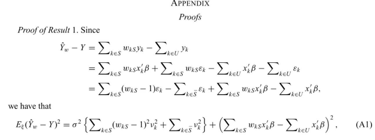
Proofs Proof of Result1. Since
ˆ Yw−Y = k∈SwkSyk− k∈Uyk =k ∈SwkSxkβ+ k∈SwkSεk− k∈Uxkβ− k∈Uεk =k ∈S(wkS−1)εk− k∈S¯εk+ k∈SwkSxkβ− k∈Uxkβ, we have that Eξ( ˆYw−Y)2=σ2 k∈S(wkS−1) 2ν2 k+ k∈S¯ν 2 k +k ∈SwkSxkβ− k∈Uxkβ 2 , (A1)
which leads to the firs equality of Result 1. The second term of (A1) can be simplified Indeed, Epk ∈SwkSxkβ− k∈Uxkβ 2 =Ep k∈SwkSxkβ−Ep k∈SwkSxkβ +Ep k∈SwkSxkβ −k ∈Uxkβ 2 =Epk ∈SwkSxkβ−Ep k∈SwkSxkβ 2 +Epk ∈UEp(wkSIk)xkβ− k∈Uxkβ 2 +2Ep k∈SwkSxkβ−Ep k∈SwkSxkβ k∈UEp(wkSIk)xkβ− k∈Uxkβ =varpk∈SwkSxkβ + k∈UCkx kβ− k∈Ux kβ 2 . (A2)
The firs term of (A1) g i v e s
σ2Epk ∈S(wkS−1) 2ν2 k+ k∈S¯ν 2 k =σ2k ∈UEp (wkS−1)2Ikνk2+ k∈U(1−πk)ν 2 k =σ2k ∈Uν 2 kEp(wkS−1)2Ik+1−πk =σ2k ∈Uν 2 k Epw2kSIk−2Ep(wkSIk)+πk+1−πk =σ2 k∈Uνk2 Epw2kSIk−E2p(wkSIk)+E2p(wkSIk)−2Ep(wkSIk)+1 =σ2 k∈Uν 2 k varp(wkSIk)+(Ck−1)2. (A3)
By the law of total variance,
varp(wkSIk)=varpEp(wkSIk|Ik)+Epvarp(wkSIk|Ik)
=πk{Ep(wkS|Ik=1)}2− {Ep(wkSIk)}2+πkvarp(wkS|Ik=1)
=1−πk
πk C
2
k +πkvarp(wkS|Ik =1). (A4)
By inserting (A4) i n t o ( A3), and by adding (A2) and (A3), we finall obtain the second equality of
Result 1.
ProofofResult 2. Result 2 comes directly from equation (2). Term B vanishes because the weights 1/πk
do not differ from sample to sample. Term C vanishes because the estimator is design-unbiased. Terms D
and Evanish because the estimator is model-unbiased under balanced sampling. All that remains is term
A with Ck = 1 because the estimator is design-unbiased.
Proof of Result3. Sinceyk=xkβ+εk, varapp( ˆYπ)= k∈Udk (yk−xkb)2 π2 k = k∈Udk εk πk − xk πk ∈Ud xx π2 −1 ∈Ud xε π2 2 =k ∈Udk ε2 k π2 k − k∈U dkxkεk π2 k ∈U dxx π2 −1 ∈U dxε π2 .
Thus, Eξ{varapp( ˆYπ)} =σ2 k∈Udk ν2 k π2 k −σ 2 k∈U ν2 k π2 k dkxk πk ∈Ud xx π2 k −1 dkxk πk .
By using the definitio of dk, given in expression (7), we obtain
Eξ{varapp( ˆYπ)} =σ2 k∈Uπk(1−πk) ν2 k π2 k =EpEξ( ˆYπ−Y) 2,
which holds even when theνkare unknown.
ProofofResult 4. The optimal inclusion probabilities πk∗are obtained by minimizing (8) subject to
k∈Uπk=n, 0πk1,
which gives the second inequality. Now, if we minimize (8) subject to k∈Uπk=n, but
with-out the constraintπk1, then we obtain πk=nνk/N, and we obtain a still lower bound in the third
inequality.
Proof of Result8. By Result 3, following the same steps, we obtain
Eξ{var( ˆˆ Yπ)} =σ2 k∈S(1−πk) ν2 k π2 k =σ2 k∈S(1−πk)2 ν2 k π2 k + k∈S¯νk2 +σ2 k∈S ν2 k πk − k∈Uνk2 =Eξ( ˆYπ −Y)2+σ2 k∈S ν 2 k πk − k∈Uν 2 k .
Obviously, if there exists a vectorλsuch thatλxk =ν2
k, then k∈S ν2 k πk − k∈Uνk2=0. REFERENCES
ARDILLY, P. (1991). ´Echantillonnage repr´esentatif optimum `a probabilit´es in´egales.Ann. D´Econ. Statist.23, 91–113. BREWER, K. R. W. (1994). Survey sampling inference: Some past perspectives and present prospects.Pak. J. Statist.
10, 15–30.
BREWER, K. R. W. (1999a). Cosmetic calibration for unequal probability sample.Survey Methodol.25, 205–12. BREWER, K. R. W. (1999b). Design-based or prediction-based inference? Stratifie random vs stratifie balanced
sampling.Int. Statist. Rev.67, 35–47.
BREWER, K. R. W. (2002).Combined Survey Sampling Inference, Weighing Basu’s Elephants. London: Arnold. BREWER, K. R. W., HANIF, M. & TAM, S. M. (1988). How nearly can model-based prediction and design-based
estimation be reconciled.J. Am. Statist. Assoc.83, 128–32.
CHAMBERS, R. L. (1996). Robust case-weighting for multipurpose establishment surveys.J. Offic Statist.12, 3–32. CUMBERLAND, W. G. & ROYALL, R. M. (1981). Prediction models in unequal probability sampling.J. R. Statist. Soc.B
43, 353–67.
DEVILLE, J.-C. (1992). Constrained samples, conditional inference, weighting: Three aspects of the utilisation of auxiliary information. InProc. Workshop on the Uses of Auxiliary Information in Surveys, pp. 21–40. ¨Orebro, Sweden: Statistics Sweden.
DEVILLE, J.-C. (1999). Variance estimation for complex statistics and estimators: Linearization and residual techniques. Survey Methodol.25, 193–204.
DEVILLE, J.-C., GROSBRAS, J.-M. & ROTH, N. (1988). Efficien sampling algorithms and balanced samples. In COMP-STAT, Proceedings in Computational Statistics, Ed. R. Payne and P. Green, pp. 255–66, Heidelberg: Physica. DEVILLE, J.-C. & S¨ARNDAL, C.-E. (1992). Calibration estimators in survey sampling.J. Am. Statist. Assoc.87, 376–82. DEVILLE, J.-C. & TILL´E, Y. (2004). Efficien balanced sampling: The cube method.Biometrika91, 893–912.
DEVILLE, J.-C. & TILL´E, Y. (2005). Variance approximation under balanced sampling.J. Statist. Plan. Infer.128, 411–25.
GODAMBE, V. P. (1955). A unifie theory of sampling from finit population.J. R. Statist. Soc.B17, 269–78. GODAMBE, V. P. & JOSHI, V. M. (1965). Admissibility and Bayes estimation in sampling finit populations I.Ann. Math.
Statist.36, 1707–22.
H´AJEK, J. (1981).Sampling from a Finite Population. New York: Marcel Dekker.
HANSEN, M. H., MADOW, W. G. & TEPPING, B. J. (1983). An evaluation of model dependent and probability-sampling inferences in sample surveys (with Discussion).J. Am. Statist. Assoc.78, 776–807.
HEDAYAT, A. S. & MAJUMDAR, D. (1995). Generating desirable sampling plans by the technique of trade-off in experimental design.J. Statist. Plan. Infer.44, 237–47.
IACHAN, R. (1984). Sampling strategies, robustness and efficien y: The state of the art.Int. Statist. Rev.52, 209–18. ISAKI, C. T. & FULLER, W. A. (1982). Survey design under a regression population model.J. Am. Statist. Assoc.77,
89–96.
KOTT, P. S. (1986). When a mean-of-ratios is the best linear unbiased estimator under a model.Am. Statist.40, 202–4. ROYALL, R. M. (1976). The linear least squares prediction approach to two-stage sampling.J. Am. Statist. Assoc.71,
657–64.
ROYALL, R. M. (1988). The prediction approach to sampling theory. InHandbook of Statistics, Vol. 6. pp. 399–413. Amsterdam, Holland: Elsevier Science Publishers.
ROYALL, R. M. (1992). Robustness and optimal design under prediction models for finit populations.Survey Methodol. 18, 179–85.
ROYALL, R. M. & CUMBERLAND, W. G. (1981). The finit population linear regression estimator and estimators of its variance. An empirical study.J. Am. Statist. Assoc.76, 924–30.
ROYALL, R. M. & HERSON, J. (1973a). Robust estimation in finit populations I.J. Am. Statist. Assoc.68, 880–9. ROYALL, R. M. & HERSON, J. (1973b). Robust estimation in finit populations II: Stratificatio on a size variable.J.
Am. Statist. Assoc.68, 891–3.
S¨ARNDAL, C.-E., SWENSSON, B. & WRETMAN, J. H. (1992).Model Assisted Survey Sampling. New York: Spinger. SCOTT, A. J., BREWER, K. R. W. & HO, E. W. H. (1978). Finite population sampling and robust estimation.J. Am.
Statist. Assoc.73, 359–61.
SMITH, T. M. F. (1976). The foundations of survey sampling: A review.J. R. Statist. Soc.A139, 183–204.
SMITH, T. M. F. (1984). Sample surveys, present position and potential developments: Some personal views (with Discussion).J. R. Statist. Soc.A147, 208–21.
SMITH, T. M. F. (1994). Sample surveys 1975–1990; An age of reconciliation (with Discussion)?Int. Statist. Rev.62, 5–34.
THIONET, P. (1953).La th´eorie des sondages. Paris: INSEE, Imprimerie Nationale. TILL´E, Y. (2006).Sampling Algorithms. New York: Springer.
VALLIANT, R., DORFMAN, A. H. & ROYALL, R. M. (2000).Finite Population Sampling and Inference: A Prediction Approach. New York: Wiley.
YATES, F. (1946). A review of recent statistical developments in sampling and sampling surveys (with Discussion). J. R. Statist. Soc.A109, 12–43.