ARENBERG DOCTORAL SCHOOL
Faculty of Engineering Science
On Constraints, Optimisation,
Probability and Data Mining
Behrouz Babaki
Dissertation presented in partial
fulfillment of the requirements for the
degree of Doctor of Engineering
Science (PhD): Computer Science
September 2017
Supervisors:
Prof. dr. Luc De Raedt
Prof. dr. Tias Guns
On Constraints, Optimisation, Probability and Data
Mining
Behrouz BABAKI
Examination committee:
Prof. dr. ir. Paul Van Houtte, chair Prof. dr. Luc De Raedt, supervisor Prof. dr. Tias Guns, supervisor Prof. dr. Patrick De Causmaecker Dr. ir. Anton Dries
Prof. dr. Siegfried Nijssen
(Université catholique de Louvain) Prof. dr. Christel Vrain
(University of Orléans)
Dissertation presented in partial fulfillment of the requirements for the degree of Doctor of Engineering Science (PhD): Computer Science
© 2017 KU Leuven – Faculty of Engineering Science
Uitgegeven in eigen beheer, Behrouz Babaki, Celestijnenlaan 200A box 2402, B-3001 Leuven (Belgium)
Alle rechten voorbehouden. Niets uit deze uitgave mag worden vermenigvuldigd en/of openbaar gemaakt worden door middel van druk, fotokopie, microfilm, elektronisch of op welke andere wijze ook zonder voorafgaande schriftelijke toestemming van de uitgever.
All rights reserved. No part of the publication may be reproduced in any form by print, photoprint, microfilm, electronic or any other means without written permission from the publisher.
Abstract
Constraint satisfaction and optimization (CSP(O)), probabilistic inference, and data mining are three important subdomains of artificial intelligence. CSP(O) investigates methods for efficiently solving combinatorial problems, probabilistic inference deals with answering queries about uncertain knowledge bases, while data mining aims at finding and modeling regularities in the data. Even though these domains have been developed independently, there are strong connections and interactions between them. Studying and extending their interactions is the main theme of this thesis.
This thesis has five contributions. First, we build on existing methods in probabilistic inference and constraint programming and propose a method for adding probabilities to the CSP(O) models. This allows us to constrain or optimize over probability values. Second, we develop a novel algorithm for optimizing the expected utility in stochastic constraint programs. Unlike earlier works that assume independence of random variables, we assume a joint distribution represented by a Bayesian network. Third, we develop an algorithm for obtaining the exact solution of the constrained clustering problem with the maximum sum of squares objective. By using the column-generation framework, we decompose the problem into two components: one that generates candidate clusters that adhere to user constraints, and one that tries to find the optimal solution among combinations of the generated candidates. Fourth, we develop an exact algorithm to solve a special class of graph clustering problems. The formulation of this problem involves an exponential number of constraints. We propose a mechanism to incrementally include only a subset of these constraints in the problem. Fifth, we develop a mechanism for learning the distribution of taxi requests from large datasets of taxi trip records.
We show that combining techniques from multiple domains can yield improvements in addressing a number of existing and new problems. We conclude by a review of directions for future work.
Beknopte samenvatting
Constraint satisfaction en optimisatie (CSP(O)), probabilistische inferentie en data mining zijn drie belangrijke subdomeinen van artificiële intelligentie. CSP(O) onderzoekt methoden om efficiënt combinatoriële problemen op te lossen, probabilistische inferentie behandelt het beantwoorden van queries betreffende onzekere knowledge bases en data mining tenslotte heeft als doel het vinden en modelleren van regelmatigheden in data. Hoewel deze domeinen onafhankelijk ontwikkeld zijn, zijn er desalniettemin sterke verbanden en interacties aanwezig. Het bestuderen en uitbreiden van deze interacties is het hoofdonderwerp van deze thesis.
Deze thesis bestaat uit vijf contributies. Ten eerste bouwen we verder op bestaande methoden in probabilistische inferentie en constraint programming en stellen we een methode voor om probabiliteiten toe te voegen aan CSP(O) modellen. Dit laat ons enerzijds toe om om te gaan met constraints op probabiliteitswaarden, anderzijds om te optimaliseren over probabiliteitswaarden. Ten tweede ontwikkelen we een nieuw algoritme om het verwachte nut in stochastische constraint programma’s te optimaliseren. In tegenstelling tot eerdere studies die onafhankelijkheid van willekeurig variabelen veronderstellen, nemen wij een gezamenlijke verdeling aan, voorgesteld door een Bayesiaans netwerk. Ten derde ontwikkelen we een algoritme om tot de exacte oplossing komen van het constrained clustering probleem met maximum sum of squares objective. Door het gebruik van het kolom-generatie framework, bereiken we een decompositie van het probleem in twee componenten: één dat kandidaat clusters, die voldoen aan constraints van de gebruiker, genereert, en één dat probeert de optimale oplossing te vinden tussen combinaties van de gegenereerde kandidaten. Ten vierde ontwikkelen we een exact algoritme om een speciale klasse van problemen op te lossen in het domein van grafenclustering. Het formuleren van dit probleem vereist een exponentieel aantal constraints. Wij stellen een mechanisme voor om op incrementele wijze slechts een subset van deze constraints te moeten beschouwen in het probleem. Ten vijfde ontwikkelen
iv BEKNOPTE SAMENVATTING
we een mechanisme om de distributie van taxiverzoeken te leren uit grote datasets van taxirit opnamen.
We tonen aan dat het combineren van technieken uit verschillende domeinen voordelen biedt bij een aantal bestaande en nieuwe problemen. We besluiten met een bespreking van mogelijke onderzoeksrichtingen voor toekomstig werk.
Acknowledgements
First, I have to thank my promoters Luc De Raedt and Tias Guns for their supervision during the course of my PhD. After five years of research, I find myself heavily influenced by their perspective. Having an established notable researcher and a rising star as promoters is a rare opportunity that I was lucky to enjoy. I am thankful to Paul Van Houtte for chairing the private and public defences. I also thank the jury members Siegfried Nijssen, Patrick De Causmaecker, Anton Dries, and Christel Vrain, for the time that they devoted to reading this thesis and providing feedback.
Even though Siegfried is not officially listed as a promoter, he has had a significant role in supervising my research, in particular with respect to the work presented in chapters 3 and 5 of this thesis. Talking to him has always been an enlightening and motivating experience, and some of the most pleasant times of my PhD were the times during which we collaborated closely.
A number of other people helped me in my research, too. The research presented in chapter 7 was conducted in collaboration with Anton. He has also answered my numerous questions on programming tools and techniques. Ever since Anton shares an office with Wannes Meert, I have divided my questions between the two of them to reduce the load. I am thankful to Guy Van den Broeck for discussions that helped me better define some of my research questions. Angelika Kimmig and Jonas Vlasselaer patiently answered my questions about probabilistic inference and probabilistic logic programming. I am also thankful to Dries Van Daele and Anna Latour for the pleasant collaboration experience that I had with them.
I started my PhD sharing an office with Anton Dries and Benjamin Negrevergne. Those who know them will confirm that how delightful it is to have the simultaneous company of them. They continued to provide a much-needed atmosphere of joy and humor for years. Sharing an office with three postdocs gave me the privilege of having access to expert advice at the first steps of my
vi ACKNOWLEDGEMENTS
research career. In those early years, on most Fridays we headed to a meeting room to discuss matters related to the ICON project. Besides Luc and Siegfried, we were accompanied by other members of the ICON team, namely Vladimir Dzyuba, Thanh Le Van, and Sergey Paramonov. I fondly remember the coffee breaks that we had right after these meetings.
Vladimir and I started our PhD almost at the same time and were in the same class of MAI program right before. During our PhD, we participated in the ICON challenge, taught exercise sessions of the data mining course, and together with Jan Van Haaren delivered a project on technology and knowledge transfer. I also enjoyed the long discussions on technical and general topics that we had on several occasions. Behind his dark humor, I found Vladimir a kind and compassionate person.
In my first year, even a short talk with Irma Ravkic, Martin Znidarsic, or Mathias Verbeke was enough to change my mood. What they shared was their big smiles and kind hearts. I owe much more than that to Irma. Being a year senior to me, she was always there to guide me through the administrative steps of my PhD.
In the final years of my PhD, I shared an office with Davide Nitti and Francesco Orsini. Sharing an office with two nice and passionate Italian colleagues is already a pleasure. In addition to that, I learned a lot from them about subsymbolic machine learning. We never ran out of topics for technical discussions. These discussions became even more interesting when another Italian fellow, Stefano Teso, joined DTAI. Francesco and I supervised a master thesis, taught the UAI exercise sessions, and together with Dimitar Shterionov and Daniele Alfarone, organized the Fluffy workshop. Thanks for all the good memories!
Speaking of subsymbolic machine learning, I have to mention thecoursera lunch
sessions that we had going for a while. Together with Golnoosh Farnadi, Geert Heyman, Tuur Leeuwenberg, Aparna Nurani Venkitasubramania and Niraj Shrestha, we learned a lot about the trendy topic of deep neural networks. Very Recently, I have been sharing office with two researchers from the latest generation of DTAI researchers: Gust Verbruggen and Arcchit Jain. I am amazed and delighted by their passion and energy. I hope that they do a better job in taking care of the office plants than what I did when Benjamin put me in charge upon his departure.
Another highlight of my last years was having lunch at the cafeteria with Jessa Bekker, Sebastijan Dumancic, Toon Van Craenendonck, Antoine Adam, Evgeniya Korneva, Vincent Vercruyssen, Pedro Miguel Zuidberg Dos Martires, Gust Verbruggen and Elia Van Wolputte. Gust and Elia also helped me by
ACKNOWLEDGEMENTS vii
translating the abstract of my thesis into Dutch.
In my difficult times over the past five years, I depended on friends that were there to hear my story and give me hope to overcome the obstacles that appeared in my way. Nasim Zand always knew how to cheer me up. Shiva Tehrani supported me during a large part of my PhD. In particular at times close to a submission deadline, I depended on her help in all matters of life. Ashkan Tabibian has done me more favors than I can ever return.
The workload of PhD research left me with little time to develop social relationships outside the department. In this situation, my close connection to two colleagues was of special value. In my first years, it was Benjamin with whom I shared my passions, frustrations, confusions and questions about research. His understanding and sympathy were always comforting. I also enjoyed his deliberately unorthodox views which were an invitation to reconsider the widely accepted traditions. I am also thankful for his so-called pearls of wisdom
which were observations about the research activity and scientific community formulated as short and amusing phrases. I found these observations quite accurate. In the later years, Jessa was the friend that I knew I can always rely on. I’m thankful to her in particular for encouraging me to take part in more social activities. A notable example was theinternational kitchen experience with some DTAI members and Nikolina Sostaric which I truly enjoyed. Above all, I am thankful to Golnoosh. From the early days of my PhD all the way to its end, she was there to hear me, sympathize with me, and encourage me. Our tea breaks and occasional lunches were the highlights of my days. I consider myself lucky to have her by my side throughout this journey.
Finally, I am thankful to my parents for constantly supporting me, especially at times that they did so despite not fully agreeing with my choices.
Contents
Abstract i
Contents ix
List of Figures xi
List of Tables xiii
1 Introduction 1
1.1 Constraint Satisfaction and Optimization . . . 1 1.2 Probabilistic Reasoning . . . 3 1.3 Data Mining . . . 4 1.4 Connections between Subdomains of Artificial Intelligence . . . 6 1.5 Contributions . . . 8 1.6 Structure of the thesis . . . 9
1.6.1 Part I: Probabilistic Models in Constraint Satisfaction and Optimization . . . 10 1.6.2 Part II: Constrained Clustering using Integer Linear
Programming . . . 11 1.6.3 Part III: Learning Taxi Passenger Demand . . . 11
2 Background 13
x CONTENTS
2.1 Bayesian Networks . . . 13
2.2 Probabilistic Inference by Knowledge Compilation . . . 15
2.3 Constraint Programming . . . 18
2.4 Mixed Integer Linear Programming . . . 20
2.4.1 Branch-and-bound search . . . 21
2.4.2 Cutting planes . . . 22
2.4.3 Column Generation . . . 23
2.5 Pattern Mining . . . 24
2.5.1 Constraint-based pattern mining . . . 25
2.5.2 Frequent pattern mining using constraint programming 26
I Probabilistic Models in Constraint Satisfaction and
Optimization
29
3 Constraint-Based Querying for Bayesian Network Exploration 30 3.1 Introduction . . . 303.2 Examples of Bayesian Network Exploration . . . 31
3.3 BN query framework . . . 33
3.4 Formulating BN Pattern Queries As Constraint Programming Problems . . . 36
3.5 Experiments . . . 39
3.6 Related work . . . 41
3.7 Conclusions . . . 42
4 Stochastic Constraint Programming with And-Or Branch-and-Bound 45 4.1 Introduction . . . 46
4.2 Stochastic Constraint Programming . . . 47
CONTENTS xi
4.4 And-Or search in a constraint solver . . . 57
4.5 Experiments . . . 58
4.6 Related work . . . 62
4.7 Conclusion and future work . . . 62
II Constrained Clustering using Integer Linear
Pro-gramming
65
5 Constrained Clustering using Column Generation 66 5.1 Introduction . . . 665.2 MSSC . . . 68
5.3 Column generation framework . . . 72
5.4 Column generation with constraints. . . 74
5.4.1 Subproblem solving . . . 75
5.4.2 Reducing the number of candidates . . . 76
5.4.3 Pruning using a bound on the objective function . . . . 77
5.5 Practical considerations . . . 79 5.5.1 Initialisation . . . 79 5.5.2 Branching . . . 79 5.5.3 Slow convergence . . . 80 5.6 Experiments . . . 80 5.7 Related work . . . 84 5.7.1 Recent developments . . . 86 5.8 Conclusions . . . 86
6 A Branch-and-Cut Algorithm for Constrained Graph Clustering 87 6.1 Introduction . . . 87
xii CONTENTS
6.3 Motivating application . . . 90
6.4 Problem and MIP formulation . . . 91
6.5 Extensions and improvements . . . 93
6.5.1 Overlapping clusters . . . 94
6.5.2 Breaking symmetries . . . 94
6.5.3 Obtaining the set of Pareto optimal solutions . . . 94
6.6 Enforcing connectivity . . . 95
6.6.1 Enumerating all simple paths . . . 96
6.6.2 A cutting plane approach . . . 96
6.7 Experiments . . . 98
6.7.1 Results and discussion . . . 100
6.8 conclusions and future work . . . 105
III Learning Taxi Passenger Demand
107
7 Feature-based Taxi Request Prediction 108 7.1 Introduction . . . 1087.2 Related work . . . 109
7.3 Problem setting . . . 111
7.3.1 Exploiting peripheral features . . . 112
7.3.2 Specificity of the model . . . 113
7.3.3 Recency of the data . . . 113
7.4 Traditional approaches . . . 114
7.4.1 Poisson processes . . . 114
7.4.2 Time-series analysis . . . 115
7.5 Feature-based taxi prediction . . . 115
CONTENTS xiii 7.5.2 Direct prediction . . . 116 7.5.3 Decomposition-based prediction . . . 117 7.6 Evaluation . . . 119 7.6.1 Data . . . 120 7.6.2 Evaluation metric . . . 121 7.6.3 Decomposition . . . 122
7.6.4 Prediction using historic data . . . 124
7.6.5 Prediction using historic data and recent observations . 126 7.6.6 Prediction on unseen regions . . . 127
7.7 Conclusions and future work . . . 129
8 Conclusions and Future Work 131 8.1 Summary and Conclusions . . . 131
8.2 Discussion and Future Work . . . 133
8.2.1 Probabilistic Models in Constraint Satisfaction and Optimization . . . 134
8.2.2 Constrained Clustering using Integer Linear Programming135 8.2.3 Learning Taxi Passenger Demand . . . 136
8.3 Concluding Remarks . . . 136
List of publications 139
Bibliography 139
List of Figures
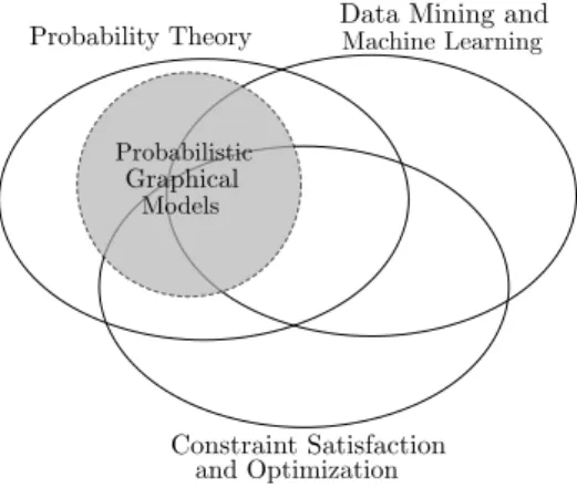
1.1 The connections between subdomains of artificial intelligence. . 2 1.2 Existing and new research on connections between multiple
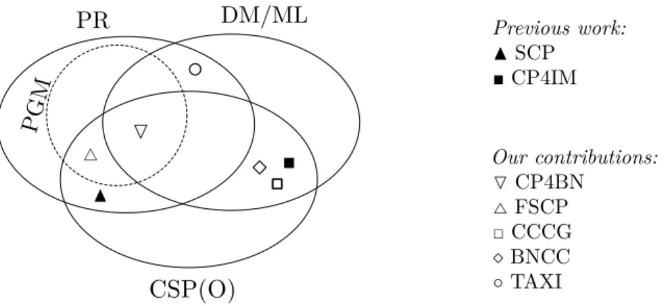
domains: Probability Theory (PR), Probabilistic Graphical Models (PGM), Data Mining/Machine Learning (DM/ML), and Constraint Satisfaction/Optimization (CSP(O)). . . 6 2.1 A Bayesian network over five variables . . . 14
2.2 Left: a Bayesian network with three variables. Right: The arithmetic circuit obtained by compiling the Bayesian network on the left (figure from (Darwiche 2009)) . . . 16
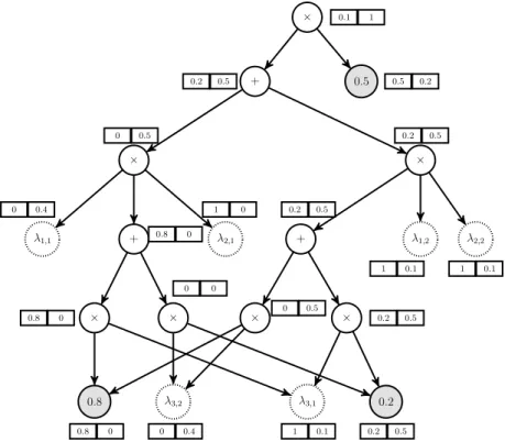
2.3 The result of circuit evaluation and differentiation for the query
P(X1 = 2, X3 = 1) by algorithm 1. The vr values are shown in
the left boxes and thedrvalues are shown in the right boxes. . . . 17
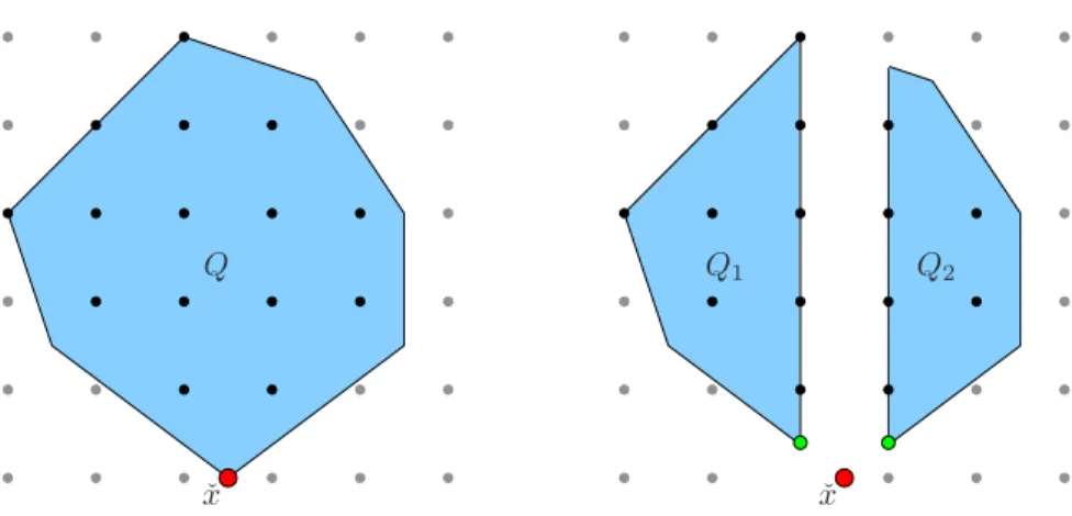
2.4 Branching decomposes problemQinto two subproblemsQ1 andQ2.
These subproblems are constructed by adding constraintsxj≤ bˆxjc
andxj≥ bˆxjctoQ. Figure from (Achterberg 2007). . . 22
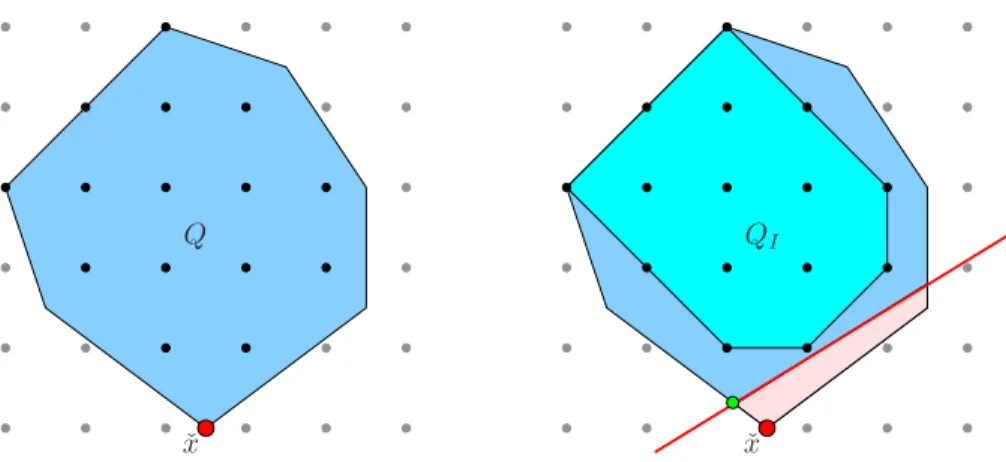
2.5 To strenghten the LP, a cut separates the solution of LP relaxation ˆx
from the convex hull of the integer program. Figure from (Achterberg 2007) . . . 23
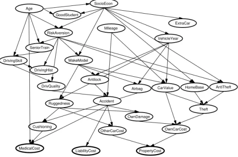
3.1 The car insurance network (Binder et al. 1997). . . 32 3.2 Arithmetic circuit for a BN with 3 variables with domain{1,2}with
X1 the parent ofX2 andX3. Square boxes represent CP variables. . 37
xvi LIST OF FIGURES
4.1 Left: Bayesian network with 2 observed and 2 hidden variables. Right: a policy tree for Example 6 with D(V1) = D(S1) =
D(V2) =D(S2) ={1,2}. . . 48
4.2 The And-Or search tree for the problem of Example 6. . . 51 4.3 Effect of depth of bounds on instances of theknapsack problem (top)
andinvestmentproblem (bottom).. . . 60
4.4 The effect of tightening theknapsackconstraint on runtime in a 6-stage problem. . . 61
5.1 Run times on the Iris data set. . . 80 6.1 Left: A small subgraph extracted from the interaction network.
Dashed lines represent the can-not-link constraints. Middle: the pathways obtained from non-overlapping clusters. Right: the pathways obtained from overlapping clusters. . . 91 6.2 The sets {2, 5} and {3, 5} belong to Γ(1,4), but the set {2, 3, 5}
does not because it is not minimal. . . 97 6.3 Impact ofγon smallest cluster size (left) and total co-occurrence
penalty (right) for instance250_750. . . 101
6.4 The Pareto optimal set for overlapping clustering on instance
250_750with three values for number of clusters. . . 102
6.5 Number of patients which are a member of each cluster, per PAM50 subtype. . . 102 6.6 Number of patients with specific PAM50 subtype, per cluster. . 104 7.1 Distribution of taxi rides for three days in February 2010: a
regular Wednesday (17/02), a regular Sunday (14/02) and a Wednesday during a blizzard (10/02). . . 112 7.2 Components discovered by NMF (c= 6). . . 119
7.3 Distribution of all trips between 5 April and 30 May 2010. Trips are aggregated to show distribution over a one week period. . . 120 7.4 Map of New York regions with high activity. . . 121
LIST OF FIGURES xvii
7.5 Average component weights for three datasets for 6 components obtained from NYC10 (components shown in Figure 7.2). SFC10 scaled up by a factor of 10. . . 123 7.6 Reconstruction error of NYC10 components by number of
components. . . 123 7.7 Prediction error for components by number of components for
List of Tables
2.1 An itemset database . . . 25 3.1 The example queries expressed using constraints over patternA. . . 34
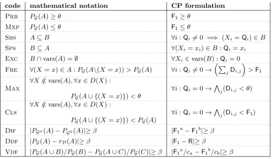
3.2 Constraints for BN pattern queries over patterns A, B, and C and network G. Constraints are represented by three-letter
codes Prb: probability(A,G, θ); Mxp: maxprobability(A,G, θ); Sbs: subset(A, B); Sps: superset(A, B); Exc: exclude(A, B); Fre: free(A,G); Max: maximal(A,G, θ); Cls: closed(A,G); Dif: difference(A,Ga,Gb, β); Ddf: DB-difference(A,G,D, β);
andVdf: ev-difference(A,G, B, C, β). . . 35
3.3 Probability queries over three benchmarks network, with#BN-n: number of BN nodes;c.Time: compilation time;#AC-n/e: number of AC nodes/edges; θ: probability threshold; #Sols: number of solutions, ands.Time: solving time. . . 40
3.4 (a) Execution times of example queries, and (b) Quality of results of sampling method as compared against the solutions of exact method.. 41
4.1 Comparing the runtime (s) of our method (AOB&B) with scenario-based approaches (CP and ILP) on the knapsack problem. The unsuccessful cases either ran out of time (T) or memory (M) during generation of scenario-based problem (G) or solving the problem (S). 58
4.2 Comparing the runtime (s) of our method (AOB&B) with scenario-based approaches (CP and ILP) on the investment problem. The unsuccessful cases either ran out of time (T) or memory (M) during generation of scenario-based problem (G) or solving the problem (S). 59
xx LIST OF TABLES
4.3 The effect of tightening theknapsackconstraint (C) on the number of nodes and failures in a 6-stage problem. . . 61
5.1 MSS clustering . . . 71 5.2 An ILP model for MSS clustering . . . 71 5.3 Dual of the optimization problem. . . 73 5.4 Model with stabilization included (N ={1, . . . , n}). . . 73
5.5 Description of datasets . . . 81 5.6 Clustering with 3 clusters and ’#c’ constraints, Iris dataset.
*optimality proven . . . 82 5.7 Clustering with 5 clusters and ’#c’ constraints, Iris dataset.
*optimality proven . . . 83 5.8 Clustering with 3 clusters and ’#c’ constraints, Wine dataset.
*optimality proven . . . 83 5.9 Clustering with 5 clusters and ’#c’ constraints, Wine dataset.
*optimality proven . . . 84 5.10 Soybean, different k and number of clusters (#c); GC gap =
difference between best solution quality of cop-kmeans and the solution of CG, INF = infeasible. . . 84 6.1 Instance properties . . . 100 6.2 Average runtimes of overlapping and non-overlapping clustering
by enumerating all simple paths (AllPaths) and branch and cut (BnC). Timed-out experiments are counted as 600 seconds (–). 103 7.1 Reconstruction error across datasets. Rows indicate components
used. Columns indicate reconstructed datasets. . . 124 7.2 sMAPE score for prediction with historic data. Results are
averaged over 11 time blocks. . . 125 7.3 sMAPE score for prediction with historic data and recent
observations. Results are averaged over 11 time blocks. . . 127 7.4 sMAPE scores for predicting on unseen regions. . . 128
Chapter 1
Introduction
Constraint satisfaction and optimization, probabilistic inference, and data mining are important subdomains of artificial intelligence, each with a long and rich history and numerous applications. Constraint satisfaction and optimization investigates methods for efficiently solving combinatorial problems, probabilistic inference deals with answering queries about uncertain knowledge bases, while data mining aims at finding and modeling regularities in the data. Despite the differences in their methods and applications, there are strong connections and interactions between these three domains. The theme of this thesis is investigating and extending such interactions. We therefore start with a brief introduction of these domains. Then we will review some of the existing work on cross-domain connections, and give an overview of the new connections that we have established in this thesis.
1.1
Constraint Satisfaction and Optimization
Aconstraint satisfaction problem (CSP) specifies a set of constraints on a set of variables. As an example, consider three variablesX1, X2, X3which can take
only values 0 or 1. The constraintX1+X2+X3≤2 restricts the values of these
variables such that their sum does not exceed 2. This problem specification in terms of variables and constraints is called amodel. To solve this CSP, one must find values for the variables such that the constraint is not violated. The valuesX1= 0, X2= 1, X3= 0 make up a solution.
A key idea in constraint satisfaction is to separate the problem specification
2 INTRODUCTION
Figure 1.1: The connections between subdomains of artificial intelligence. from the mechanism that finds the solution. An implementation of such a solving mechanism is called asolver. The advantage of this separation is that it offers a declarative approach for solving a problem: the user only needs to specify the problem as a model, and the solver will take care of finding the solution.
The central principles employed in constraint programming solvers aresearch
andpropagation. Search is an enumerative procedure that assigns values to a variable from its domain. Propagation is a means for reducing the number of values that are examined during search (i.e. the search space). It involves removing values from the domain of a variable by reasoning over a constraint that includes that variables and domains of other variables in that constraint. In a CSP, any assignment that respects the constraints is a valid solution. If some solutions are preferred to others, we can define a score for solutions and ask for the solutions with the highest score. This gives aconstraint optimization problem (COP), which is a CSP together with anobjective function that maps each solution to a real number.
Standard constraint programming solvers can solve COPs using thebranch and bound method. If the constraints and the objective function are linear, and the variables are integer or continuous (e.g. the knapsack problem), then we have a
mixed integer linear programming (MILP) problem.There are solvers dedicated to finding the optimal solution for MILP problems. The key principle in these solvers is to use a relaxed version of the problem to obtain bounds during search. This relaxed problem which is obtained by dropping the integrality condition is a linear program and can be solved efficiently.
PROBABILISTIC REASONING 3
Knapsack Problem
Given a set of items and their weights and values, we want to collect a subset of them such that the total weight of collected items does not exceed the capacity of our knapsack, and their total value is maximized. We can formulate this problem as a COP:
max.X i viXi s.t. X i wiXi≤C Xi∈ {0,1} ∀i
The binary variableXi encodes our decision about taking or leaving item
i. The constantsvi andwi represent the value and weight of itemi. The
objective function P
iviXi is equal to the total value of collected items,
and the constraintP
iwiXi≤Censures that the total weight of collected
items does not exceed the capacityC.
Finding an exact solution for an optimization problem can be difficult. An alternative to exact search is to useapproximation algorithmsorheuristicsthat produce near-optimal solutions at a lower computational cost. An approximation algorithm is accompanied by a bound on the ration between the near-optimal and optimal solutions. There is no such theoretical guarantee for heuristic search methods, and their effectiveness is evaluated empirically. In this thesis we follow the convention of AI community in using the termapproximatefor any method that does not produce exact solutions.
1.2
Probabilistic Reasoning
It is well known that reasoning only based on deterministic facts and rules is not enough to address the challenges of the real world, largely due to their inherently uncertain nature. A response to this problem is to use probability theory as a basis for reasoning under uncertainty. In general, this is a difficult task as it can involve visiting an exponential number of possibilities. However, there
4 INTRODUCTION
Bayesian Network
A Bayesian network is a directed acyclic graph that represents a probability distribution. To each node in the network corresponds a conditional probability of that node given its parent nodes. The Bayesian network models the joint distribution over all nodes as the product of these conditional probabilities. The figure below shows a small Bayesian network.
P(Rain,Sun,Rainbow) =
P(Rain)×P(Sun|Rain)×
P(Rainbow|Sun,Rain)
Rain Sun
Rainbow
There are inference algorithms for answering probability queries in Bayesian networks, such as P(Rainbow=True) andP(Rain=False,Sun=False).
These algorithms use independence relationships in the Bayesian network to improve the efficiency in calculation of probability values.
are representations that allow for efficient probabilistic reasoning. Probabilistic graphical models are a class of such representations that can encode conditional independence relations between groups of random variables. The reasoning algorithms use these independencies to decompose the problem into subproblems that can be solved independently. Depending on the structure of the distribution, this can lead to significant computational savings. One of the most-studied types of probabilistic graphical models areBayesian networks. In this thesis, we mostly focus on these models.
1.3
Data Mining
Data mining (DM) is concerned with discovering knowledge from data. In different data mining tasks, the discovered knowledge can have different forms. The two data mining tasks that we deal with in this thesis are pattern mining and clustering. In pattern mining, the user is interested in finding substructures that appear regularly in the data. In clustering, the discovered knowledge is presented as a grouping of data instances into a number of clusters.
DATA MINING 5
Frequent Itemset Mining
Consider a database of transactions where each transaction consists of a set of items. In the toy database on the right, the first to third transac-tions are{B},{E}, and{A, C}. The
problem of frequent itemset mining is to find subsets of items (called itemsets) that are included in at least as many transactions as a given threshold. A B C D E 0 1 0 0 0 0 0 0 0 1 1 0 1 0 0 1 0 0 0 1 0 1 1 0 0 0 0 0 1 1 0 0 1 1 1 1 1 1 0 0 1 1 0 0 1 1 1 1 0 1
Some of the frequent itemsets for threshold 2 in this toy database are∅, {E}, {B, C}, and {A, B, E}. If we add the constraint that the itemsets
must contain at least two items, the itemsets∅ and{E} will be excluded.
The goal in the task offrequent pattern mining is to find substructures that appear more than a certain number of times in the data. Extensive research has been conducted on efficient algorithms for finding frequent patterns of different types.
Usually the large number of discovered frequent patterns makes it difficult for the user to analyze them. This has motivated the research on methods for reducing these results to a smaller set of patterns. Constraint-based pattern mining reduces the number of output patterns by requiring the patterns to satisfy extra constraints other than frequency. Another approach is to use
condensed representations which means to eliminate the redundancies in the discovered patterns.
Clustering is a descriptive data mining task. The goal in clustering is to create a model of the data in terms of groups that constitute it. The clustering algorithms aim to group the data into clusters that have certain properties. One such property that is common to most clustering algorithms is that the members of a cluster are similar to each other and different from the members of other clusters.
The desired properties of clusters can be represented in terms of constraints. A
must-link constraint between two data instances requires that these instances belong to the same cluster. A can-not-link constraint forbids such a co-membership. Another example is thesizeconstraint which restricts the number
6 INTRODUCTION
of members of a cluster.
1.4
Connections between Subdomains of Artificial
Intelligence
The connections between constraint satisfaction and optimization (CSP(O)), probabilistic inference, and DM/ML have been studied before. Figure 1.2 positions our work in relation to the domains of AI and these cross-domain studies. In this thesis, we propose alternative frameworks for adding probabilistic models to CSP(O) formulations. Our aim is to exploit both probabilistic and deterministic structures in solving these problems. Our work on pattern mining in Bayesian networks (CP4BN in figure 1.2) links three topics of DM/ML, CSP(O), and PGM. In our work on factored stochastic constraint programming (FSCP in figure 1.2), we build on an existing work on stochastic constraint programming (SCP in figure 1.2) which combined CSP(O) with probabilities(Walsh 2002).
We contribute to topics at the intersection of CSP(O) and DM by formulating and solving mining and learning tasks using integer linear programming and constraint programming. Our two works on clustering (CCCG and BNCC in figure 1.2) are a continuation of a trend on combining DM/ML and CSP(O). This trend was initiated by a framework (CP4IM in figure 1.2) for solving
Previous work: NSCP CP4IM Our contributions: OCP4BN 4FSCP CCCG BNCC ◦ TAXI
Figure 1.2: Existing and new research on connections between multiple domains: Probability Theory (PR), Probabilistic Graphical Models (PGM), Data Mining/Machine Learning (DM/ML), and Constraint Satisfaction/Optimization (CSP(O)).
CONNECTIONS BETWEEN SUBDOMAINS OF ARTIFICIAL INTELLIGENCE 7
itemset mining problems by constraint programming (Guns et al. 2011b). We also extend this framework to pattern mining in Bayesian networks. Finally, in our work on learning taxi passenger demand (TAXI in figure 1.2), we learn probabilistic models from the data using standard methods in statistical machine learning.
The matter of combining optimization and probabilistic inference has been studied in the uncertainty reasoning community, for example under the topic of influence diagrams. However, constraint processing has not received much attention in these studies. Such a combination has been also studied in the constraint programming community. But it is common practice in these studies to either assume that the random variables are independent (Walsh 2002) or to sample scenarios from the probability distribution and combine them into a single deterministic constraint program (Manandhar et al. 2003). The former method assumes strict independence relationships and the latter approach (calledscenario-based stochastic constraint programming) ignores the structure of the probability distribution. Sampling scenarios has been also a successful approach for solving stochastic vehicle routing problems (Bent and Hentenryck 2004).
Research at the intersection of DM and CSP(O) has a natural motivation. At the core of data mining tasks usually lies a search in a hypothesis space for finding all/best hypotheses according to some criteria. The standard practice for finding these hypotheses is to develop search algorithms that are targeted at that specific learning or mining problem. The search space can be discrete or continuous, and the algorithms can be approximate or exact.
An alternative approach for solving these problems is to formulate them as CSP(O) models. This approach has multiple advantages: 1) Moving away from developing algorithms to formulating the problem in a certain language, makes it easier to rapid-prototype new ideas. 2) Once a good formulation for a task is developed, variants of it can be obtained by modifying the constraints and/or the objective function. 3) Advances in constraint solving technologies translate into improvements in mining and learning tasks.
There are successful examples of using this principle in continuous domain, such as using mathematical programming solvers for solving the underlying optimization problem in support vector machines (Schölkopf et al. 2000). Recently, there has been an interest in using the same approach for problems with a combinatorial search space. Several pattern mining tasks have been formulated as constraint satisfaction problems and solved using standard constraint programming solvers (Guns et al. 2011b; Guns et al. 2011a; Négrevergne and Guns 2015). A similar approach (although using other constraint solving frameworks) has been applied to tasks such as structured-output prediction (Teso
8 INTRODUCTION
et al. 2017) and inference in statistical relational learning (Riedel 2008). An area in DM where using CSP(O) has been popular is constraint-based learning and mining. In constraint-based learning, the space of valid hypotheses is expressed in terms of constraints. An example of using CS for constraint-based supervised learning is structure learning of Bayesian networks, which has been formulated using integer linear programming (Bartlett and Cussens 2017). In constrained clustering, which is an example of unsupervised constraint-based learning, the desired properties of clusters are expressed through constraints. By formulating the clustering problem as a constraint programming model, a wide range of such properties can be enforced by adding extra constraints to the base model (Dao et al. 2017).
Similarly, in constraint-based pattern mining, the desired properties of patterns are described by constraints such asfrequency andclosedness. When a pattern mining task is modeled as a constraint solving problem, such constraints can be enforced by adding extra constraints, or modifying the existing ones (Guns et al. 2011b).
1.5
Contributions
This thesis has three parts. In each part we study the connections between a number of domains in artificial intelligence. In the first part we present mechanisms for integrating constraint programming and probabilistic inference. In the second part, we evaluate the potential of integer linear programming for the task of constrained clustering. In the third part we investigate a learning problem which is part of a stochastic optimization pipeline. The research questions that are answered in each of the three parts are:
Q1How can we use probabilistic graphical models within CSP(O) formulations? Q2What is the potential of formulating constrained clustering as integer linear
programming problems?
Q3How can we use data mining techniques to learn the distribution of passenger
requests from records of taxi trips?
The contributions of this thesis with respect to questionQ1are as follows:
• We developed a way to represent the results of probability queries as variables in a CSP model. This method uses existing technologies in probabilistic inference and constraint programming. This method allows solving CSP(O) problems that have constraints or objective functions that
STRUCTURE OF THE THESIS 9
are defined in terms of the result of a probability query. We illustrate this technique by applying it to a novel data mining task, namely constraint-based pattern mining in Bayesian networks.
• We developed a novel algorithm for optimizing the expected utility in constraint programs which have probabilistic parameters. These parameters can have a joint distribution represented by a Bayesian network. We developed a novel bounding mechanism that takes advantage of the probabilistic structure. Our method outperforms the existing algorithms for solving such problems.
The contributions obtained in this thesis with respect to questionQ2are the
following:
• We developed an algorithm for obtaining the exact solution for the constrained clustering problem with the maximum sum of squares (MSS) objective. This algorithm is based on formulating the clustering problem as an integer linear program and solving it by using the column generation method. Our algorithm supports a set of constraints that are common in constrained MSS clustering.
• Motivated by a data mining application, we developed an exact algorithm to solve a special class of graph clustering problems. We developed two integer linear programming formulations of this problem. Our solution methods are efficient enough for finding the optimal solution of real-world instances that motivated this problem.
Finally, we have the following contribution with respect to questionQ3:
• We developed a mechanism for learning the distribution of taxi requests from large datasets of taxi trip records. In our experiments, the model obtained through this mechanism outperformed the existing approaches.
1.6
Structure of the thesis
We first present the background material inChapter 2. This chapter provides
the background on a number of topics that are used in the subsequent chapters, namely constraint programming, integer linear programming, and inference in graphical models.
The structure of rest of the thesis follows the three research questions formulated above. The three parts of this thesis are as follows:
10 INTRODUCTION
1.6.1
Part I: Probabilistic Models in Constraint Satisfaction
and Optimization
Chapter 3introduces the new problem of pattern mining in Bayesian networks.
Similar to (Guns et al. 2011b), we use constraint programming to formulate the problem. One difference between pattern mining in Bayesian networks and in databases is that in the former the input is represented intensionally in a compact form. Instead of unfolding this compact form into its extensional equivalent, we use knowledge compilation to compile this distribution into an intermediate structure which is then embedded in a constraint program as a set of constraints. This chapter has been previously published in the following paper:
• Behrouz Babaki, Tias Guns, Siegfried Nijssen, and Luc De Raedt. “Constraint-based querying for bayesian network exploration”. In Élisa
Fromont, Tijl De Bie, and Matthijs van Leeuwen, editors, Advances in Intelligent Data Analysis XIV - 14th International Symposium, IDA 2015, Saint Etienne, France, October 22-24, 2015, Proceedings,volume 9385 of
Lecture Notes in Computer Science,pages 13–24. Springer, 2015.
Chapter 4presents a new flavor of stochastic constraint programming. In this
setting, the joint distribution of random variables is represented by a Bayesian network. Hence we deal with a deterministic and a probabilistic structure. Existing methods can only exploit one of these two structures. We exploit both structures by combining two computational tasks of probabilistic inference and constraint satisfaction in an And-Or search tree. This chapter is based on the following paper:
• Behrouz Babaki, Tias Guns, and Luc De Raedt. “Stochastic constraint programming with and-or branch-and-bound”. In Carles Sierra, editor,
Proceedings of the Twenty-Sixth International Joint Conference on Artificial Intelligence, IJCAI 2017, Melbourne, Australia, August 19-25, 2017, pages 539–545. ijcai.org, 2017.
1.6.2
Part II: Constrained Clustering using Integer Linear
Programming
The two chapters in this part present applications of CSP(O) in DM.
Chapter 5The goal in this chapter is to use integer linear programming for
STRUCTURE OF THE THESIS 11
exponential in the number of data instances. We show that this problem can be solved by adding the variables to the model in a lazy fashion. This results in a hybrid scheme that allows us to deal with a subset of constraints in a subproblem outside the integer programming workflow. This chapter is previously published in this paper:
• Behrouz Babaki, Tias Guns, and Siegfried Nijssen. “Constrained clustering using column generation”. In Helmut Simonis, editor,Integration of AI and OR Techniques in Constraint Programming - 11th International Conference, CPAIOR 2014, Cork, Ireland, May 19-23, 2014. Proceedings,
volume 8451 of Lecture Notes in Computer Science, pages 438–454. Springer, 2014.
Chapter 6 deals with a clustering problem where the relations among data
instances are represented as a graph. A key requirement in this problem is that the subgraphs induced by the clusters must be connected. We formulate this problem as an integer linear program, and express the connectedness property as a set of constraints. Since the number of these constraints is exponential in the size of input graph, we solve the problem by including only a sufficient subset of these constraints. This chapter is published in this paper:
• Behrouz Babaki, Dries Van Daele, Bram Weytjens, and Tias Guns. “A branch-and-cut algorithm for constrained graph clustering”. Data Science meets Optimization workshop (colocated with CPAIOR), Padova, Italy, 2017.
1.6.3
Part III: Learning Taxi Passenger Demand
Chapter 7deals with the problem of learning the passenger request for taxi
trips. The motivation for learning this model is to produce samples to be used by a scenario-based algorithm for the stochastic routing problem. In this chapter we study the problem of learning such distributions from large amounts of data. This chapter is based on the following work:
• Behrouz Babaki, and Anton Dries. Feature-based Taxi Request Prediction.
(manuscript in preparation).
Finally,Chapter 8concludes this thesis by presenting a summary, conclusions
Chapter 2
Background
This chapter provides the background on probabilistic graphical models, constraint programming, integer programming and constraint-based pattern mining.
2.1
Bayesian Networks
The idea in probabilistic reasoning is to use probability theory to reason over uncertain beliefs. This requires the belief to be represented as a probability distribution. However, the number of possible worlds grows exponentially in the number of entities that one holds a belief about. This immediately poses a challenge both in terms of representation and reasoning. In the general case, one will need to visit all these possibilities and assign a probability to each one. Similarly, at inference time all these possibilities need to be enumerated. Probabilistic graphical models address this problem using a basic insight. Usually, theconditional independenciesprovide significant information about beliefs. The language of graphs can easily represent these independencies. Using these models, it is sufficient to specify these independences as a graph, and only specify the probability distribution for each factor. Bayesian networksare one of the most popular types of probabilistic graphical models.
Definition 1. A Bayesian network G is a directed acyclic graph where each
node represents a random variable Xi in X ={X1, . . . , Xn}. Let PaGXi denote the parents ofXi inG. A joint distributionP over the set of variablesX is said
to factorize according to G if P(X1, . . . , Xn) can be expressed as the product
14 BACKGROUND Winter? (A) Sprinker? (B) Rain?(C) Wet Grass?
(D) Slippery Road?(E)
A P1(A) 0 0.4 1 0.6 A B P2(B|A) 0 0 0.25 0 1 0.75 1 0 0.8 1 1 0.2 A C P3(C|A) 0 0 0.9 0 1 0.1 1 0 0.2 1 1 0.8 A C D P4(D|B, C) 0 0 0 1 0 1 0 0 0 0 1 0.2 0 1 0 0.8 1 0 0 0.1 1 1 0 0.9 1 0 1 0.05 1 1 0 0.95 C E P5(E|C) 0 0 1 0 1 0 1 0 0.3 1 1 0.7
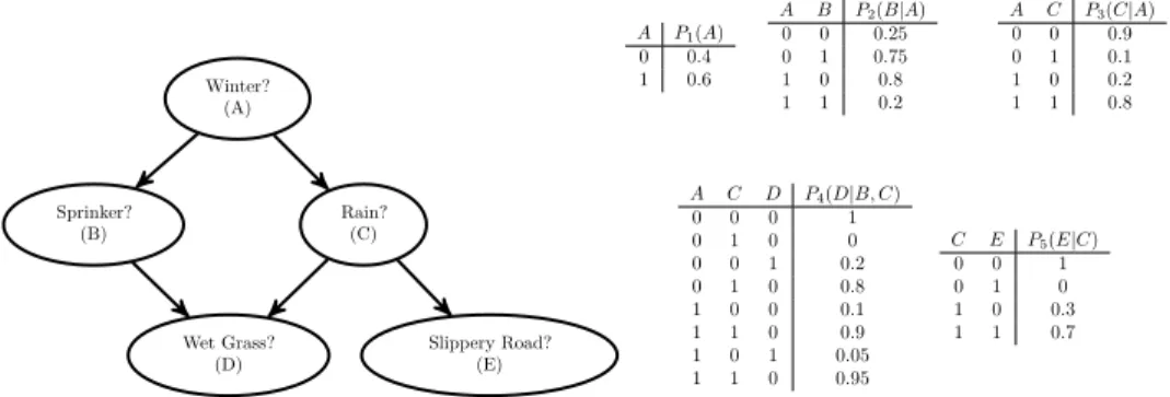
Figure 2.1: A Bayesian network over five variables
Qn
i=1P(Xi|PaXGi). We denote the distribution factored according toG by PG. We denote by D(Xi) the domain of variable Xi, that is, the possible values
the variable can take. An assignment of valuexi to variableXi is denoted by
(Xi =xi).
The joint probability of variables in a Bayesian network is fully specified by its graph and the distributionsP(Xi|PaGXi). When the variables are discrete,
each of these distributions can be represented extensionally as a conditional probability table (CPT) (Pearl 1989).
A probabilistic query is a question about probability of events according to a distribution. These queries are answered byprobabilistic inference algorithms. There are several types of such algorithm (for a detailed discussion of these algorithms, see (Darwiche 2009)). The common principle among them is to take advantage of the conditional independencies to decompose the inference problem.
Example 1. Consider the graph in figure 2.1. It shows that the joint probability
of random variablesA, B, C, D, E factorizes as follows:
P(A, B, C, D, E) =P1(A)·P2(B|A)·P3(C|A)·P4(D|B, C)·P5(E|C)
The joint probability distribution is fully described by this graph and the conditional probability tables for P1, . . . , P5. The query P(A= 1)in example 1
PROBABILISTIC INFERENCE BY KNOWLEDGE COMPILATION 15
can be decomposed and solved as follows:
P(A=true) = X B,C,D,E P(A= 1, B, C, D, E) = X B,C,D,E P1(A= 1)·P2(B|A= 1)·P3(C|A= 1)·P4(D|B, C)·P5(E|C) = X B,C,D P1(A= 1)·P2(B|A= 1)·P3(C|A= 1)·P4(D|B, C)· X E P5(E|C) | {z } =1 =X B,C P1(A= 1)·P2(B|A= 1)·P3(C|A= 1)· X D P4(D|B, C) | {z } =1 =X B P1(A= 1)·P2(B|A= 1)· X C P3(C|A= 1) | {z } =1 =P1(A= 1)· X B P2(B|A= 1) | {z } =1 =P1(A= 1) = 0.6
2.2
Probabilistic Inference by Knowledge
Compila-tion
One of the methods for inference in Bayesian networks is to first compile it to anarithmetic circuit and then evaluate the query on the circuit. Compilation is an offline step and has to take place only once for each network. The resulting circuit can be used for answering multiple queries (Darwiche 2003).
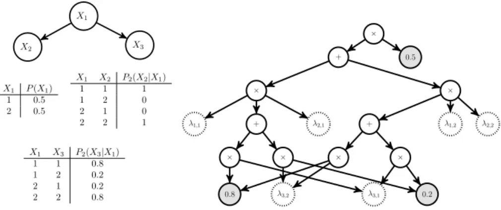
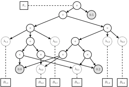
Consider the Bayesian network in left side of figure 2.2. Compiling this network results in the circuit depicted in the right side of the figure. We will now see how this circuit can be used to answer probability queries. The circuit has two types of leaves: parameterswhich are set according to the probability values in the network CPTs, and theλvariables, which are calledindicators. The indicator
16 BACKGROUND X1 X2 X3 X1 P(X1) 1 0.5 2 0.5 X1 X2 P2(X2|X1) 1 1 1 1 2 0 2 1 0 2 2 1 X1 X3 P2(X3|X1) 1 1 0.8 1 2 0.2 2 1 0.2 2 2 0.8 + 0.5 × × + + λ1,2 λ2,2 λ1,1 λ2,1 × × × × λ3,2 λ3,1 0.8 0.2 ×
Figure 2.2: Left: a Bayesian network with three variables. Right: The arithmetic circuit obtained by compiling the Bayesian network on the left (figure from (Darwiche 2009))
variables are set according to the query that the user wants to evaluate. Once these variables are set, the circuit can be evaluated using a bottom-up pass. For each variable Xi and valuej ∈D(Xi) there exists an indicator variable
denoted byλij. To evaluate the queryP(Xi1 =j1, . . . , Xik =jk), the indicator
variables should be set as follows:
• If a variable is assigned to a value in the query, set the indicator variable corresponding to that assignment to 1, and those corresponding assignment to other values of that variable to 0. For example in the query above, the indicator variables λi1,j1 should be set to 1 and all otherλi1,j forj6=j1
should be set to 0.
• If a variable is not mentioned in the query (i.e. it is marginalized over), the indicator variables corresponding to all values of this variable should be set to 1.
Figure 2.3 shows how the queryP(A= 1, C= 0) is evaluated.
An arithmetic circuit can be seen as a function f over indicator variables.
Consider a partial assignmentA, Bayesian network variableXi and the value
j∈D(Xi). It has been shown that the following equality holds:
∂f ∂λi,j( A) = ( P(A∪ {(Xi=j)}) ifXi is not assigned inA P(A\{(Xi=k)})∪ {(Xi=j)}) if (Xi=j)∈A
PROBABILISTIC INFERENCE BY KNOWLEDGE COMPILATION 17
It has also been shown that the derivatives off with respect to allλij variables
can be computed in a single top-down pass. Algorithm 1 shows how the value off and its derivatives are computed in two passes through the circuit. It takes
the arithmetic circuitAC and two arraysvr anddrfor storing the value and
derivative in each node. The value and derivative corresponding to nodev in
the circuit are represented byvr(v) anddr(v). It is assumed that the values of
leaf nodes are initialized invr(v). Let us denote the root node of the circuit by r. The function TwoPasscomputes the value of circuit output in thevr(r). It
also computes the derivatives of leaf nodesv indr(v). The computed derivatives
for the circuit of figure 2.2 are shown in figure 2.3.
+ 0.5 0.2 0.5 0.5 0.2 × 0.5 0.2 × 0.5 0 + 0.5 0.2 + 0.8 0 λ 2,2 0.1 1 λ1,2 0.1 1 λ1,1 0.4 0 λ2,1 0 1 × 0 0.5 × 0 0 × 0.2 0.5 × 0 0.8 λ3,2 0.4 0 λ3,1 0.1 1 0.8 0 0.8 0.2 0.5 0.2 × 0.1 1
Figure 2.3: The result of circuit evaluation and differentiation for the queryP(X1=
2, X3= 1) by algorithm 1. Thevrvalues are shown in the left boxes and thedrvalues
18 BACKGROUND
Algorithm 1 Evaluating and differentiating an arithmetic circuit (from
Darwiche 2009)
1: functionTwoPass(AC, vr, dr)
2: foreach circuit nodev(visiting children before parents)do 3: compute the value ofvand store it invr(v)
4: end for
5: dr(v)←0 for all non-root nodesv
6: dr(r)←1 . ris the root node
7: foreach circuit nodev(visiting parents before children)do 8: foreach parentpof nodevdo
9: if pis an addition nodethen 10: dr(v)←dr(v) +dr(p)
11: else
12: dr(v)←dr(v) +dr(p)Q
v06=vvr(v 0
), wherev0 is a child of parentp
13: end if
14: end for
15: end for
16: end function
2.3
Constraint Programming
Constraint programming is an instance of thedeclarative programmingparadigm. Like other declarative methods, in constraint programming the user only specifies the problem and not the solution method. Constraint programming systems are equipped with solvers that decide how to search for solutions to the given problem. A constraint satisfaction problem is a triple (V, D,C) in which V is a
set of variables,Dis a set of domains which map every variablev∈ V to a set
of valuesD(v), andCis a set of constraints which further limit values fromD
that can be assigned toV (F. Rossi et al. 2006).
Example 2. We have three items with weights 10, 15, and 20. Each item has
a value. The values of these three items are 5, 1, and 10. We want to pick two of these items while respecting the following conditions: 1) The sum of weights of selected items should not exceed 35, and 2) If we pick the first item, we can not select the third one.
To formulate this problem in constraint programming, we introduce discrete variables x1,x2, andx3 as indicators for selection of each of three items. We
also introduce the real variables which represents the total weight of selected
items. SoV ={x1, x2, x3, s}. The domain of discrete variables is the finite set
{0,1}, and the domain of continuous variable is the interval[0,45]. In other
CONSTRAINT PROGRAMMING 19
consists of following constraints:
x1+x2+x3= 2 (2.1)
s= 10x1+ 15x2+ 20x3 (2.2)
s≤35 (2.3)
(x1= 1)→(x3= 0) (2.4)
Constraint 2.1 reflects that we want to pick exactly two items. Constraint 2.2 specifies that sis sum of selected items. Constraints 2.3 and 2.4 reflect the two
conditions specified in the problem description1.
The two main operations of a constraint solving system are search and propagation. Search is the act of trying different values (or ranges of values)
for variables. For discrete variables, this is done by assigning values from the domain of that variable. For continuous variables, search is done by partitioning the domain into disjoint intervals. The intervals that have a size smaller than a predefined precision will not be partitioned anymore.
Propagation is the act of removing values (or ranges) from the domain of variables that given the domains of other variables and the model constraint, cannot be part of a solution. Given a constraint c defined over variables x1, . . . , xn with domainsD1, . . . , Dn, we define the set of admissible values for
variablex1 as:
{a1∈D1:∃a2∈D2, . . . ,∃an∈Dn such thatC(a1, . . . , an) holds}
For continuous variables, the propagation mechanism computes a superset, namely the smallest interval enclosing this set.
Example 3. Consider a simple model consisting of three continuous variables x1, x2, andy with domains[a, b], [c, d], and[−∞,∞], respectively. Propagation
according to the constrainty=x1+x2 will reduce the domain of variabley to
[a+c, b+d]. If we replace this constraint byy=x1∗x2, the domain ofy will
be reduced to [min(ac, ad, bc, bd), max(ac, ad, bc, bd)].
If we reduce the domains of variables in a CSP in such a way that all constraints hold for each value in the domain of each variable, we have found a solution for that CSP.
1This problem can be modeled without using continuous variables. However, we have
20 BACKGROUND
Example 4 (Example 2 continued). For solving the problem formulated in
example 2, we start by assigning value 1 for x1. This assignment, together
with constraint 2.2 triggers a propagation step which reduces the domain ofs
to[10,45]. A similar propagation step based on constraint 2.4 removes value 1
from the domain ofx3. This in turn changes the domain ofs to[10,25]. We
continue by assigning value 0 to x2. As a result, the domain of s reduces to
[10,10]. At this point, all variables are assigned a value from their domain, and
all constraints hold for these values. This means that we have found a solution.
Note that in the previous example, we did not have to search for the value of
s, as its value was determined by propagation. In other words, our previous
assignments to other variables, dictated thatsshould be equal to 10.
Global constraints A global constraint is a constraint over a non-fixed number
of variables. Global constraint are often semantically redundant; meaning that they can be represented by a set of simpler constraints. However, a global constraint provides better access to the structure of the problem. A famous example is thealldifferent(x1, . . . , xn) constraint which enforces
that each pair of variables x1, . . . , xn should take different values. Consider alldifferent(x1, x2, x3). This constrain can be replaced by three inequality
constraints x1 6= x2, x1 =6 x3, x2 6= x3. Now consider a situation where the
domain of all three variables is {1,2}. The alldifferent constraint can
reason over these domains and issue a failure. However, the inequality constraints do not have access to this global view and can not detect the failure.
Constraint optimization Aconstraint optimizationproblem is a CSP together
with a functionf defined overV. The goal is to find a solutionS∗ such that f(S∗)≤f(S) for all solutionsS to the problem. This problem can be solved
using a CSP solver using a simple procedure. Initially a solutionS is obtained
by backtracking search. Then the constraintf(V)< Sis added to the constraint
setC. Solving this problem will give a solution with a smaller objective function.
These steps are repeated until no solution is found. The solution obtained last is optimal.
2.4
Mixed Integer Linear Programming
Amixed integer linear programming(MILP) problem is a constraint optimization problem with linear constraints and objective function. This class of optimization problems has been extensively studied and sophisticated solvers have been
MIXED INTEGER LINEAR PROGRAMMING 21
developed for solving this type of problems (Achterberg 2007). These problems can contain both integer and continuous variables. A MILP problem can be specified by the tuple (A, b, c, I) whereA∈Rm×n is the coefficient matrix,b∈ Rmis the right-hand-side vector,c∈Rnis the cost vector, andI⊆ {1, . . . , n}is
the set of indices of integer variables. The vector of decision variables is denoted byx. By definition,xj∈Z,∀j∈I andxj ∈R,∀j /∈I. Further restrictions on
domains of variables can be specified as bound constraintslj≤xj ≤uj which
are a special case of linear constraints. The problem is to find values forxj
variables from their domains such that the objective functioncTxis minimized
and the constraintsAx≤bhold.
Given a constraint optimization problemP, a relaxationPR is an optimization
problem such that each solution of P is a valid solution for PR. A linear
programming (LP) relaxation of a MILP problem is obtained by turning the integer variables into continuous variables. This gives a linear programming problem that can be solved efficiently. MILP solvers heavily rely on solving these LP relaxations. These solvers employ a range of sophisticated mechanisms. We will review the two most important mechanisms, namely branch-and-bound search and the cutting planes method.
2.4.1
Branch-and-bound search
As indicated by its name, branch-and-bound search relies on two principles.
Branching is the practice of dividing a problem into smaller instances. In MILP solvers, these subproblems are generated by adding constraints to the base problem. Note that the disjunction of these constraints should not remove any solutions from the base problem. This process resembles the search in CSP solvers. Theboundingmechanism is employed in order to avoid the enumeration of all solutions of a problem. During the search, the smallest objective value among all discovered solutions up to that moment produces an upper bound. If the lower bound for a subproblem exceeds this upper bound, that subproblem can be safely ignored. The lower bound is obtained by solving the LP relaxation of the subproblem. An important factor that determines the strength of this bound is how close the constraints of the relaxed problem are to the original constraints. Thestrengthof an LP relaxation is the degree to which this holds. Besides providing a bound, the LP relaxation can also guide the branching decisions. The most-commonly used branching strategy in MILP solvers is to pick an integer variablexj which has a fractional value ˆxj in the solution of
the LP relaxation. The two branches are created by adding the constraints