Machine Learning in Adversarial Environments

(1)

Machine Learning in Adversarial Environments

by

Chaowei Xiao

A dissertation submitted in partial fulfillment of the requirements for the degree of

Doctor of Philosophy

(Computer Science and Engineering) in the University of Michigan

2020

Doctoral Committee:

Professor Mingyan Liu, Chair Professor Atul Prakash Professor Jason Corso

Assistant Professor David Fouhey Assistant Professor Bo Li

(2)

Chaowei Xiao [email protected]

ORCID iD: 0000-0002-7043-4926 © Chaowei Xiao 2020

(3)

Dedication

This manual is dedicated to all doctoral students at the University of Michigan’s Horace H. Rackham School of Graduate Studies.

(4)

Acknowledgments

I would like to start with thanking my parents for unconditional supports. Thanks for their open-minded attitude towards me. I will never forget their sacrifice to ensure me to receive a quality education. Their selfless love and never-failing affectionate support have made me overcome the difficulties and pursue my academic dream.

I was very lucky to be a student advised by Professor Mingyan Liu. I am grateful for her providing me this valuable opportunity to work with her and giving me enough freedom, support, and encouragement for my research career. Beyond the tremendous and detailed advice that she has given on my professional career, she also taught me how to analyze the problem and how to build up the personal research taste. I am really grateful that she gave me enough time to study the fundamental knowledge and courses during my first two years instead of involving in a lot of research projects. I still remembered that the countless days and nights she has been spent on our research projects. Even she has become the chair of the ECE department, she still could sacrifice her lunchtime or spare time to talk with me. Additionally, she also offered me a lot of help in my personal life. I still remembered that she told me to sync with her frequently during the year when I was visiting at UC Berkeley because she hoped to confirm that I was safe and studying enjoyably instead of my research progress. She also provides me unconditional supports during the time of my job searching. She gave me enough time and freedom to prepare my job materials and spent a lot of time to help me revise the materials and rehearsal. Even after the interview process, she also helped me analyze the advantages and drawbacks of each offer and replied to my message during the mid-night. The work presented in this dissertation would not have been possible without her.

I am also extremely grateful to professor Bo Li. She provided me the precise and detailed advice and spent countless hours on my research and showed enough patient. I am so grateful to her recommendation of being a visiting student at UC Berkeley at Professor Dawn Songs group and also providing me the opportunity for academic services. Without her help and advice, the work presented in this dissertation would never come out.

I am also extremely thankful to professor Dawn Song. She provided me the opportunity to visit UC Berkeley and enough resources. I spent a really fruitful and wonderful time in her group.

I am also extremely grateful to professor Yunhao Liu, who was my advisor of my undergraduate university. I am thankful to his support and recommend me to join professor Mingyan Lius group. Never shall I forget the unconditional support and enough encouragement he provided. In the

(5)

meanwhile, I am also grateful to professor Lei Yang and Zheng Yang, who was my advisors of my undergraduate university as well.

I am also extremely grateful to professor Alfred Chen, professor Jia Deng, professor Jie Gao, professor Yang Liu, and professor Ning Zhang. They provided me a lot of support during my application for the academic position.

Special thanks to my close collaborators who made this thesis possible. I would like to thank Dawei Yang. He provided me a lot of help on 3D adversarial projects. I appreciate his many useful suggestions and patience during our collaboration. I would like to thank Warren He for his help on the projects of digital adversarial examples. I will never forget his inspiration and enthusiasm. I am looking forward to seeing the success of the mobile app he developed. I would like to thank Ruizhi Deng for his help on defense projects. He helped me conduct a huge amount of experiments. I would like to thank Yulong Cao for his help on LiDAR project. He taught the details of autonomous driving systems. He also provided me a lot of help when we first organized a workshop in CVPR. Over the summers, I have had the fortune to intern with many researchers, including Denis Weng and Yu Chen at JD.COM, Ian Molloy and Taesung Lee at IBM Research, Hamid Palangi, Lei Zhang, Houdong Hu and Jianfeng Gao at Microsoft Research. I appreciate these opportunities provided by them.

I would also like to thank all of my other collaborators: Alfred Chen, Yulong Cao, Hongge Chen, Jia Deng, Ruizhi Deng, Tudor Dumitras, Kevin Eykholt, Ivan Evtimov, Earlence Fernanes,Kevin Fu, Jie Gao, Cho-Jui Hsieh, Warren He, Mo Li, Xiang-Yang Li, Kin Sum Liu, Yang Liu, Yunhao Liu, Honglake Lee, Ian Molloy, Xinlei Pan, Atul Prakash, Haonan Qiu, Amir Rahmati, Armin Sarabi, Liang Tong, Jian Tang, Yevgeniy Vorobeychik, Chenshu Wu, Gang Wang, Xinyu Xing, Zheng Yang, Lei Yang, Dawei Yang, Fisher Yu, Xinchen Yan, Ning Zhang, Ziyun Zhu, Huan Zhang, and Junyan Zhu. Thanks for your great efforts and help. Without your help and efforts, the work in this dissertation would never appear.

I would like to thank my labmates Xueru Zhang, Armin Sarabi, Yang Liu, Parinaz Naghizadeh, Mohammad Mahdi Khalili, Mehrdad Moharrami, Kun Jin, Chenlan Wang.

Finally, I would also like to thank my committee members Atul Prakash, Jason Corso, David Fouhey, and Bo Li. I am grateful to them for the valuable comments and suggestions for my dissertation.

(6)

LIST OF FIGURES

FIGURE

2.1 Overview of AdvGAN . . . 9 2.2 Generating adversarial examples with spatial transformation: the blue point denotes

the coordinate of a pixel in the output adversarial image and the green point is its corresponding pixel in the input image. Red flow field represents the displacement from pixels in the adversarial image to pixels in the input image. . . 11 2.3 Adversarial examples generated from the same original image to different targets by

AdvGAN and stAdv on MNIST. We use the format ”model — attack method” to label the subcaption. On the diagonal, the original images are shown. . . 14 2.4 Comparison of adversarial examples generated by FGSM, C&W and stAdv. (Left:

MNIST, right: CIFAR-10) The target class for MNIST is “0” and “air plane” for CIFAR-10. We generate adversarial examples by FGSM and C&W with perturbation bounded in terms ofL₁as 0.3 on MNIST and 8 on CIFAR-10. . . 14 2.5 Adversarial examples generated by AdvGAN on CIFAR-10 and ImageNet. For the

left image, the image from each class is perturbed to other different classes and the original images are shown on the diagonal. For the right image, images shown on the first column are the original images. The following columns are the corresponding adversarial examples which are classified as (from left to right) poodle, ambulance, basketball, and electric guitar. . . 15 2.6 Adversarial examples generated by stAdv against different models on CIFAR-10. The

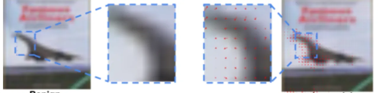
ground truth images are shown in the diagonal while the adversarial examples on each column are classified into the same class as the ground truth image within that column. 16 2.7 Flow visualization on MNIST. A digit “0” is misclassified as “2”. . . 16 2.8 Flow visualization on CIFAR-10. An “airplane” image is misclassified as “bird”. . . . 17 2.9 Flow visualization on ImageNet. (a): the original image, (b)-(c): images are

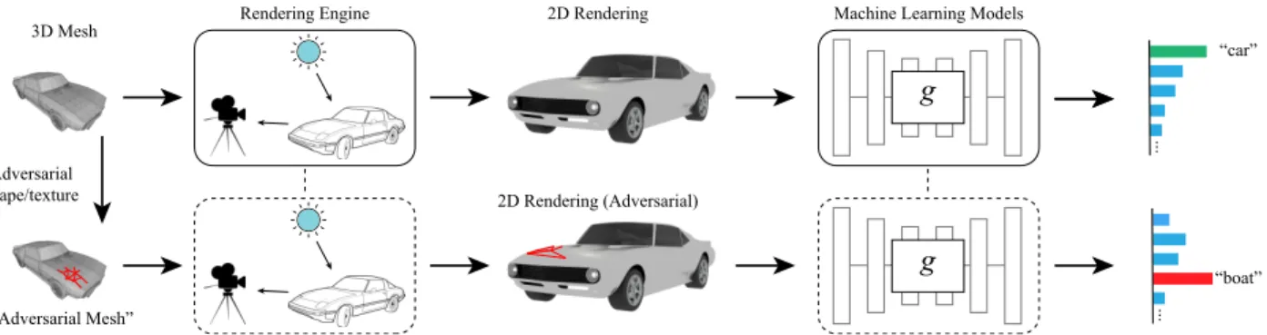
misclassi-fied into goldfish, dog and cat, respectively. Note that to display the flows more clearly, we fade out the color of the original image. . . 17 3.1 The pipeline of “adversarial mesh” generation by meshAdv. . . 22 3.2 Benign images (diagonal) and corresponding adversarial examples generated by

me-shAdv onPASCAL3D+ renderingstested on Inception-v3. Adversarial target classes are shown at the top. We show perturbation on (a) shape and (b) texture. . . 29

(9)

3.3 Benign images (diagonal) and corresponding adversarial examples generated by me-shAdv onPASCAL3D+ renderingstested on Inception-v3. Adversarial target classes are shown at the top. We show perturbation on (a) shape and (b) texture. . . 30 3.4 (a) and (b) are visualization of shape based perturbation with respect to Figure 3.2(a).

(c) is a close view of flow directions, and (d) is an example to compare the magnitude of perturbation with the magnitude of curvature. Warmer color indicates greater magnitude and vice versa. . . 31 3.5 “Adversarial meshes” generated by meshAdv in a synthetic indoor scene. (a) represents

the benign rendered image and (b)-(e) represent the rendered images from “adver-sarial meshes” by manipulating the shape or texture. We use the format “adver“adver-sarial target|perturbation type” to denote the victim object aiming to hide and the type of

perturbation respectively. . . 33 3.6 “Adversarial meshes” generated by meshAdv for an outdoor photo. (a) and (c) show

images rendered with pristine meshes as control experiments, while (b) and (d) contain “adversarial meshes” by manipulating the shape. We use the format “S/Sadv|target”

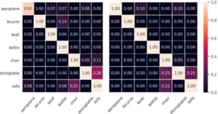
to denote the benign/adversarial 3D meshes and the target to hide from the detector respectively.. . . 34 3.7 Confusion matrices of targeted success rate for evaluating transferability of “adversarial

meshes” on different classifiers.Left: DenseNet;right: Inception-v3. . . 35 3.8 Transferability of “adversarial meshes” against classifiers in unknown rendering

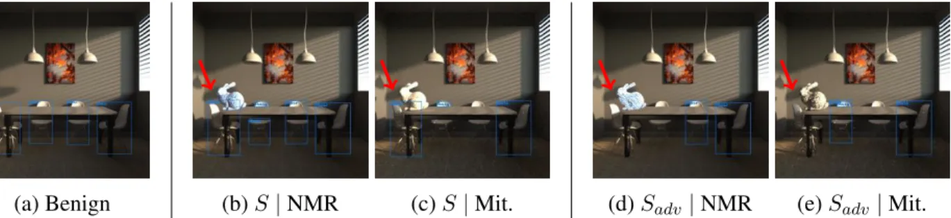
envi-ronment. We estimate the camera viewpoint and lighting parameters using the differen-tiable renderer NMR, and apply the generated “adversarial mesh” to the photorealistic renderer Mitsuba. The “airliner” is misclassified to the target class “hammerhead” after rendered by Mitsuba. . . 36 3.9 Transferability of “adversarial meshes” against object detectors in unknown rendering

environment. (b) (c) are controlled experiments. Sadv _{is generated using NMR (d),}

targeting to hide the leftmost chair (see red arrows), and the adversarial mesh is tested on Mit. (Mitsuba) (e). We use “S/Sadv_|_{renderer” to denote whether the added object}

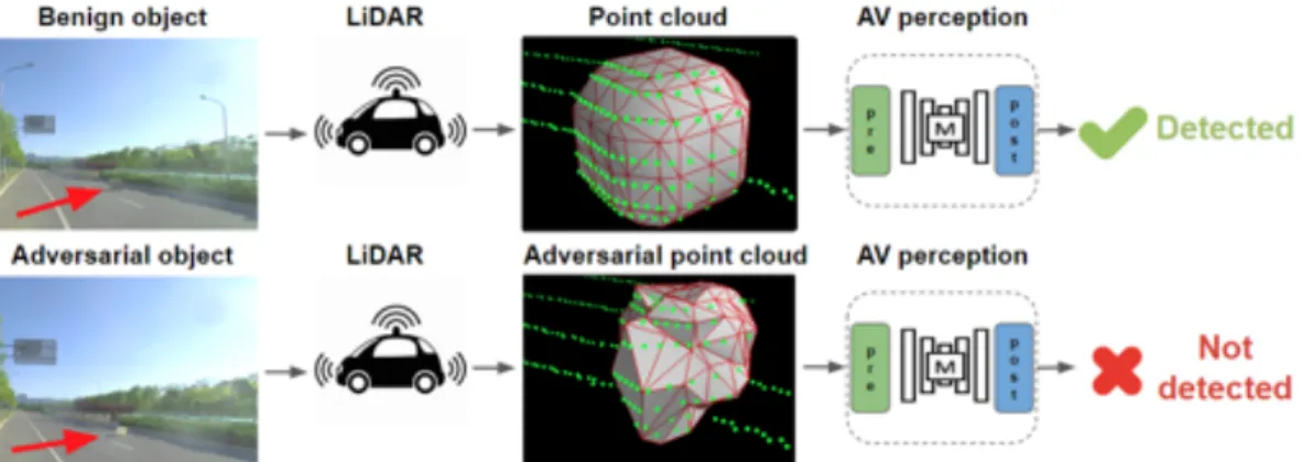
is adversarially optimized and the renderer that we aim to attack with transferability respectively. . . 36 4.1 Overview of LiDARadv. The first row shows the control experiment where a regular

box is detected by the LiDAR-based detection system; row 2 shows the generated adversarial object with similar size cannot be detected. . . 38 4.2 Overview of LiDAR-based detection on AV. . . 39 4.3 The performance of trilinear approximator and tanh approximator. The format“ (_·)00

count

represents the 2D count feature calculated by trilinear approximator 0_;_M₍ 0₍_X₎₎

obj

represents visualization of the “objectiveness ” metric in the output of modelM using trilinear approximator with; 0₍_X₎

count - (X)count represents the approximator ’s

error of 0_{. The same notation for tanh approximiator} 00 _{. . . 44} 4.4 Adversarial meshes of different sizes can fool the detectors even with more LiDAR

hits. We generate the object with LiDARadv and evolution-based method (Evo.). . . . 47 4.5 The adversarial mesh generated by LiDARadv is mis-detected as a “Pedestrian”. . . . 48

(10)

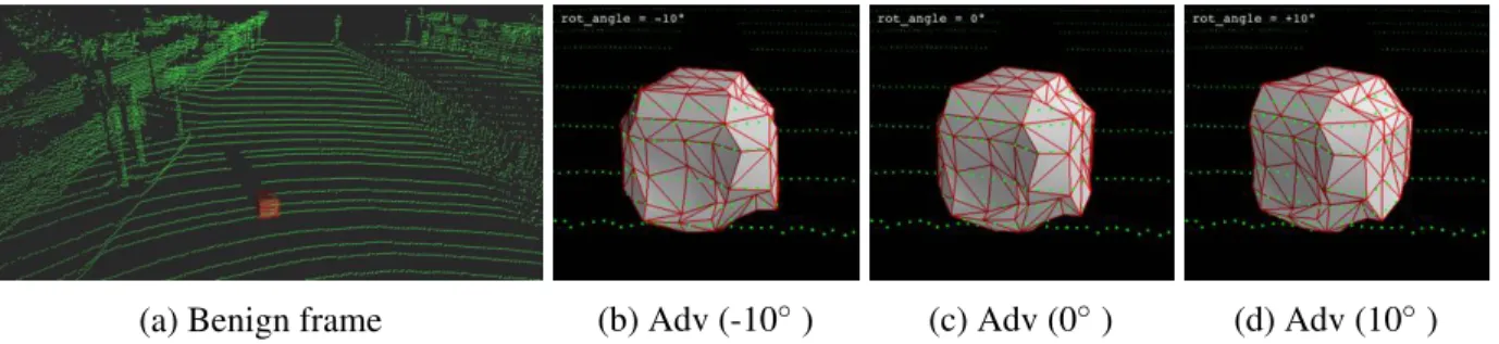
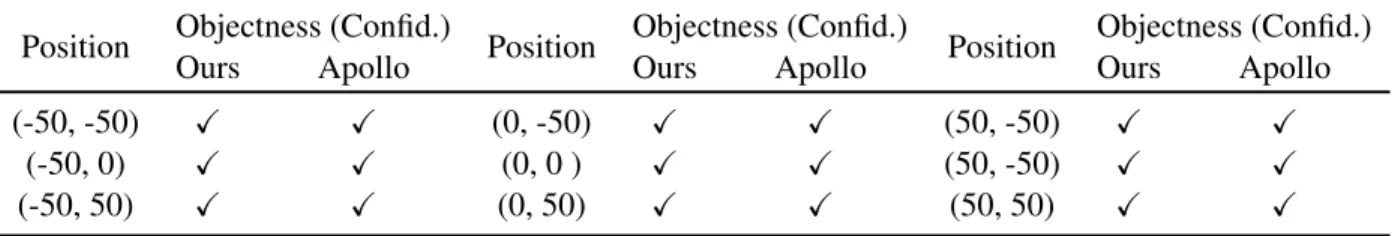
4.6 The visualization of the adversarial object with different angles. In the benign frame (a), the system is able to detect the cube. When we replace the cube with our adversarial object, the system fails to detect the object at all three angles. We visualize the mesh along with the point clouds in a close-up view in (b), (c) and (d). . . 49 4.7 Our adversarial object can successfully attack the detection system, while placed at

different positions. The red spheres mark the locations we place the adversarial object. 50 4.8 The optimized robust adversarial objects from 6 principal views and a particular view,

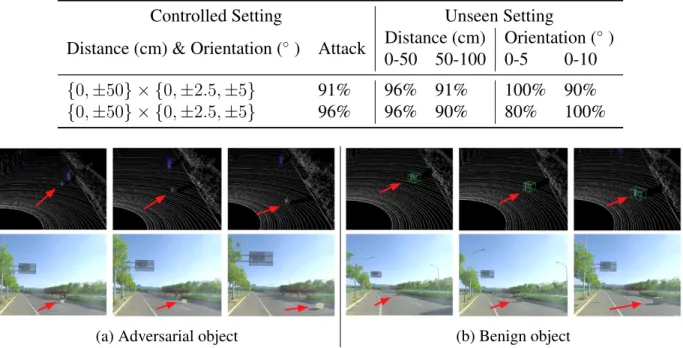
compared with the original pristine object.. . . 50 4.9 Results of physical attack. Our 3D-printed robust adversarial object by LiDARadv is

not detected by the LiDAR-based detection system in a moving car. Row 1 shows the point cloud data collected by LiDAR sensor, and Row 2 presents the corresponding images captured by a dash camera.. . . 51 4.10 Our physical experiment setting. We 3D-print the generated adversarial object at 1:1,

and drive a car mounted with LiDAR and dashcams to collect the scanned point clouds and the reference videos. . . 52 5.1 Spatial consistency analysis for adversarial and benign instances in semantic

segmenta-tion. . . 55 5.2 Samples of benign and adversarial examples generated by Houdini on Cityscapes

(targeting on Kitty/Pure) and BDD100K (targeting on Kitty/Scene). We select DRN as our target model here. Within each subfigure, the first column shows benign images and corresponding segmentation results, and the second and third columns show adversarial examples with different adversarial targets. . . 56 5.3 Heatmap of per-pixel self-entropy on Cityscapes dataset against DRN model. (a) and

(b) show a benign image and its corresponding per-pixel self-entropy heatmap. (c)-(f) show the heatmaps of the adversarial examples generated by DAG and Houdini attacks targeting “Hello Kitty” (Kitty) and random pure color (Pure). . . 56 5.4 Examples of spatial consistency based method on adversarial examples generated by

DAG and Houdini attacks targeting on Kitty and Pure. First column shows the original image and corresponding segmentation results. ColumnP1 andP2 show two randomly

selected patches, while columnO1and O2 represent the segmentation results of the

overlapping regions from these two patches, respectively. The mIOU betweenO1and

O2 are reported. It is clear that the segmentation results of the overlapping regions

from two random patches are very different for adversarial images (low mIOU), but relatively consistent for benign instance (high mIOU). . . 57 5.5 Examples of images and corresponding segmentation results before/after image

scal-ing on Cityscapes against DRN model. For each subfigure, the first column shows benign/adversarial image, while the later columns represent images after scaling by applying Gaussian kernel with std as 0.5, 3, and 5, respectively. (a) shows benign images before/after image scaling and the corresponding segmentation results; (b)-(e) present similar results for adversarial images generated by DAG and Houdini attacks targeting on Kitty and Pure. . . 60

(11)

5.6 Performance of adaptive attack. (a) shows adversarial image and corresponding seg-mentation result for adaptive attack against image scaling. The first two rows show benign images and the corresponding segmentation results; the last two rows show the adaptive adversarial images and corresponding segmentation results under different std of Gaussian kernel (0.5, 3, 5 for column 2-4). (b) and (c) show the performance of adaptive attack against spatial consistency based method with differentK. (b) presents mIOU of overlapping regions for benign and adversarial images during along different iterations. (c) shows mIOU for overlapping regions of benign and adversarial instances at iteration 200. . . 63 5.7 Detection performance of spatial consistency based method against adaptive attack with

differentK on Cityscapes with DRN model. X-axis indicates the number of patches selected to perform the adaptive attack (0 means regular attack). Y-axis indicates the number of overlapping regions selected for during detection. . . 64 5.8 Transferability analysis: cell(i, j)shows the normalized mIoU value or pixel-wise

attack success rate of adversarial examples generated against modelj and evaluate on modeli. Model A,B,C are DRN (DRN-D-22) with different initialization. We select “Hello Kitty” as target . . . 65 6.1 Pipeline of the proposed temporal consistency based adversarial frame identifier: AdvIT . 68 6.2 Benign and adversarial frames generated on Cityscapes and Davis Challenge 17 dataset

for video segmentation and human pose estimation respectively. . . 69 6.3 Benign and adversarial frames generated on MPII and UCF-101 for video object

detection and action recognition respectively. . . 70 6.4 Benign and adversarial frames generated on MPII and UCF-101 for action recognition. 70 6.5 Heatmap of per-pixel cross-entropy. (a) and (b) show a benign frame and the

corre-sponding per-pixel cross entropy between the prediction of its pseudo frames and itself. The rest show similar per-pixel cross entropy for adversarial frames with different targets. The labels indicate their adversarial targets. . . 73 6.6 Examples of consistency measurement based onAdvIT for various video tasks. The

first column indicates previous Frames. The second column indicates the current frame and corresponding prediction result. The last column indicates a sampled pseudo frame and corresponding prediction. The consistency metricC shows quantitative results for different learning tasks. Note that higherC for segmentation and object detection means higher consistency, while lowerCindicates more consistent for Human pose estimation since it is based onL2 distance. . . 74

A.1 Samples of benign and adversarial examples. We use the format “attack method —at-tack model — dataset” to label the settings of each adversarial examples. Within each subfigure, the first column shows benign images and corresponding segmenta-tion results, the second and third columns show adversarial examples with different adversarial targets (targeting on Kitty/Pure in (a),(c), (d) and on Kitty and Scene in (b),(d),(f)). . . 85 A.2 Attack results of additional targets on Cityscapes. The first column shows benign

instance, while 2-4 columns show adversarial examples with target “ECCV 2018”, “Remapping”, and “Color strip”, respectively. . . 86

(12)

A.3 Heatmap of per-pixel self-entropy. (a), (b), (g), (h), (m) and (n) show benign images and its corresponding per-pixel self-entropy heatmaps. We use the format “examples — attack model — dataset” to label them. For the rest, we use the format “attack method — target label — attack model — dataset” to label each subcaption. . . 90 A.4 Examples of images and corresponding segmentation results before/after image

scal-ing. For each subfigure, the first column shows benign/adversarial images, while the following columns represent images after scaling by applying Gaussian kernel with std as 0.5, 3, and 5, respectively. (a),(f) and (k) show benign images before/after image scaling and the corresponding segmentation results and we use the format “example — attack model — dataset” to identify the corresponding model and dataset; (b)-(e), (g)-(j) and (l)-(o) present similar results for adversarial images and we use the format “attack method — target label — attack model — dataset” to label the settings of each

image. . . 92 A.5 Examples of images and corresponding segmentation results for adaptive attack against

image scaling. For each subfigure, the first column shows benign/adversarial images, while the following columns show images after scaling by applying Gaussian kernel with std as 0.5, 3, and 5, respectively. (a), (f), (k) and (p) show benign images before/after image scaling and the corresponding segmentation results and The format “example — attack model — dataset” uses to identify the corresponding model and dataset; (b)-(e), (g)-(j), (l)-(o) and (q)-(t) present similar results for adaptive adversarial images and we describe by the format “attack method — target label — attack model — dataset”. . . 95 A.6 Detection performance of spatial consistency based method against adaptive attack

with differentK. We use the format “attack model — target label — dataset” to label the settings for each figure. X-axis indicates the number of patches selected to perform the adaptive attack (0 means regular attack). Y-axis indicates the number of overlapping regions selected during detection. We select the minimal mIOU from benign patches as our threshold on Cityscapes, and the one which guarantees accuracy as above 95% on benign images for BDD. . . 98 A.7 Transferability analysis on CityScapes dataset: cell(i, j)shows the normalized mIoU

value or pixel-wise attack success rate of adversarial examples generated against model j and evaluate on modeli. Model A,B,C have the same architecture (DRN-C-26 or DLA34UP) with different initialization. We use format “attack method|attack target|

model ” to denote the caption of each sub-figure. . . 100 A.8 Transferability analysis on BDD dataset. . . 102 A.9 Transferability visualization on CityScapes dataset. In each sub-figure, the first row

presents the segmentation results of adversarial example on model A (targeted model) and model B. The second row shows the adversarial target and the ground truth. We use format “attack method|attack target|model ” to denote the caption of each sub-figure.103 A.10 Transferability visualization on BDD dataset. . . 105

(13)

A.11 Transferability analysis for classification models: cell(i, j)shows the attack success

rate of the adversarial examples generated against Modelj and evaluate on Model iunder targeted attack setting. Model A,B,C are model with the same architecture (DRN-D-22, DRN-C-26 or DLA34UP) and different initialization. All the adversarial examples are generated using fast iterative gradient sign method. The caption of each sub-figure bear the “dataset|model”. . . 106

(14)

LIST OF TABLES

TABLE

2.1 Comparison with the state-of-the-art attack methods. Run time is measured for gener-ating 1,000 adversarial instances during test time. C&W represents the optimization based method, and Trans. denotes black-box attacks based on transferability. . . 8 2.2 Accuracy of different models on pristine data, and the attack success rate of adversarial

examples generated against different models by AdvGAN on MNIST and CIFAR-10. . 13 2.3 Accuracy of different models on pristine data, and the attack success rate of adversarial

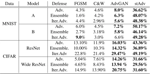
examples generated against different models by stAdv on MNIST and CIFAR-10. . . 13 2.4 Attack success rate of adversarial examples generated by AdvGAN and stAdv under

defenses on MNIST and CIFAR-10. . . 19 3.1 Attack success rate of meshAdv and average distance of generated perturbation for

different models and different perturbation types. We choose rendering configurations inPASCAL3D+ renderingssuch that the models have 100% test accuracy on pristine meshes so as to confirm the adversarial effects. The average distance for shape based perturbation is computed using the 3D Laplacian loss from Equation 3.12. The average distance for texture based perturbation is the root-mean-squared error of face color change. . . 28 3.2 Targeted attack success rate for unseen camera views. We attack using 5, 10, or 15

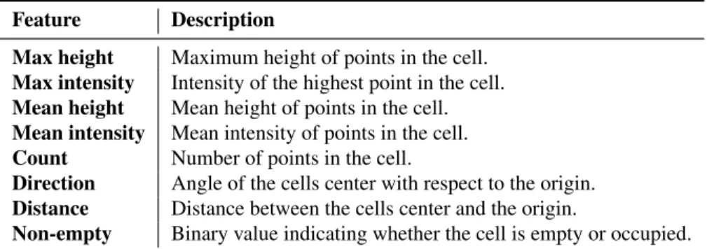
views, and test with 20 unseen views in the same range. . . 32 3.3 Untargeted attack success rate against Mitsuba by transferring “adversarial meshes”

generated by attacking a differentiable renderer targeting different classes. . . 35 4.1 Machine learning model input features extracted in the preprocessing phase.. . . 40 4.2 Output metrics of the segmentation model. . . 40 4.3 Attack success rate of LiDARadv and evolution based method under different settings. 48 4.4 The attack success rate of the adversarial objects generating using LiDARadv, starting

from different types of pristine meshes. The target labels are the other four labels different from the original predictions. . . 48 4.5 Robust Adversarial Object against different angles. The original confidence is x. Our

success rate is 100%. (Xrepresents no object detected) . . . 49 4.6 Robust Adversarial Object against different positions. The original object can be

(15)

4.7 Attack success rates of LiDARadv at different positions and orientations under both

controlled and unseen settings. . . 51

5.1 Detection results (AUC) of image spatial (Spatial) and scale consistency (Scale) based methods on Cityscapes dataset. The number in parentheses of the Model shows the number of parameters for the target mode, and mIOU shows the performance of segmentation model on pristine data. We color all the AUC less than 80% with red. . . 62

6.1 Comparison of detection results (AUC) against different attacks for AdvIT and baseline methods. . . 77

6.2 Detection results (AUC) againsttemporal continuity attack . . . 78

6.3 Detection results (AUC) of adaptive attacks and transferability analysis. . . 79

6.4 Detection overhead ofAdvIT (in seconds). . . 80

A.1 Detection results (AUC) of image spatial (Spatial) and scale consistency (Scale) based methods on BDD dataset. The number in parentheses of the “Model” shows the number of parameters for the target mode, and “mIOU” shows the performance of segmentation model on pristine data. We color all the AUC less than 80% with red. . . 87

A.2 Detection results (AUC) of image spatial (Spatial) based method with random patch size on Cityscapes dataset. . . 88

A.3 Detection results (AUC) of image spatial (Spatial) based method with random patch size on BDD dataset. . . 88

A.4 Detection results (AUC) of spatial consistency (Spatial) based method on Cityscapes dataset for additional targets. . . 88

A.5 Detection results (AUC) of spatial consistency (Spatial) based method on BDD dataset for additional targets. . . 89

B.1 Detection results (AUC) ofAdvIT againstindependent frame attackon various video tasks with different attack methods and targets. . . 109

B.2 Accuracy of the predicted pseudo-frames among different settings . . . 110

(16)

ABSTRACT

Machine Learning, especially Deep Neural Nets (DNNs), has achieved great success in a variety of applications. Unlike classical algorithms that could be formally analyzed, there is less understanding of neural network-based learning algorithms. This lack of understanding through either formal methods or empirical observations results in potential vulnerabilities that could be exploited by adversaries. This also hinders the deployment and adoption of learning methods in security-critical systems.

Recent works have demonstrated that DNNs are vulnerable to carefully crafted adversarial perturbations. We refer to data instances with added adversarial perturbations as “adversarial examples”. Such adversarial examples can mislead DNNs to produce adversary-selected results. Furthermore, it can cause a DNN system to misbehavior in unexpected and potentially dangerous ways. In this context, in this thesis, we focus on studying the security problem of current DNNs from the viewpoints of bothattackanddefense.

First, we explore the space of attacks against DNNs during the test time. We revisit the integrity ofLp regime and propose a new and rigorousthreat modelof adversarial examples. Based on this new threat model, we present the technique to generate adversarial examples in the digital space.

Second, we study the physical consequence of adversarial examples in the 3D and physical spaces. We first study the vulnerabilities of various vision systems by simulating the photo taken process by using the physical renderer. To further explore the physical consequence in the real world, we select the safety-critical application of autonomous driving as the target system and study the vulnerability of LiDAR-perceptual module. These studies show the potentially severe consequences of adversarial examples and raise awareness on its risks.

Last but not least, we develop solutions to defend against adversarial examples. We propose a consistency-check based method to detect adversarial examples by leveraging property of either the learning model or the data. We show two examples in segmentation task (leveraging learning model) and video data (leveraging the data), respectively.

(17)

CHAPTER 1 Introduction

Background Machine Learning, especially Deep Neural Networks (DNNs), has achieved great success in many applications [26,48,50,70,74]. The essence of most ML tasks is to approximate an unknown mapping from an input domain to an output domain given samples of input-output pairs. To obtain this mapping function, ML algorithms are proposed. These algorithms usually split the data into two sets:training datawith both input and output (label) domain information andtest datawith only input domain information. They learn the mapping function using the training data and are then applied to the test data to assess their accuracy. These algorithms are developed based on a strong assumption that the distribution of the training data is similar to the distribution of the test data. However, this assumption introduces potential problems.

First of all, when we randomly sample data into a training set and a test set, it may introduce sampling bias (out-of-distribution data in the test set), which can be hard to eliminate and results in uncertain prediction results. More importantly, this assumption is built upon a benign environment free of adversarial manipulation in either the training data or the test data. In practice, there exist many incentives for data manipulation, some adversarial in nature, due to the wide deployment of DNNs system in a variety of safety-critical applications, such as spam detection and autonomous vehicles. For instance, spam detection is one of the first widely used application which employs machine learning to detect spam [34]. It did not take long for attackers to launch evasion attacks through content manipulating to evade detection and send spam [34]. In this thesis, we aim to study such security problems of modern DNNs by discovering and fixing identified vulnerabilities in adversarial environments where an attacker could perform adversarial manipulation.

Within this context, two types of security threats have been defined based on when adversarial manipulations are performed. An attack during the training stage is called a poisoning attack, while one during the test stage an evasion attack (or adversarial machine learning). In this thesis, we focus on the latter, the security threats on the test stage where parameters of a DNN are fixed.

The robustness of a targeted DNN. is typically evaluated/tested using generated input instances called adversarial examples. These adversarial examples are designed to lead to erroneous and undesirable output by the target DNN, but deemed harmless or ineffective when used on humans.

(18)

The problem of generating such adversarial examples is formalized as follows: Given a learned classifierf :_X _!_Y from an input domain_X (e.g. image) to a set of classification outputs_Y (e.g. label), an adversary aims to generate an adversarial examplexadv for an original instancex₂ _X with its ground truth labely ₂ _Y, so that the classifier predictsf(xadv) ₆= y(untargeted attack) orf(xadv) =t(targeted attack) wheretis the target class, while a typical human can easily (and correctly) recognizef(xadv)asy.

Adversarial examples have been shown to subvert malware detection, fraud detection, or even potentially mislead autonomous navigation systems [38,43,95], and therefore pose security risks when applied to security-critical applications. A comprehensive study on adversarial examples is required to enable effective defense and to develop safe and reliable machine learning systems. Motivation One important criterion for adversarial examples in the digital space is that the perturbed input should “look like” the original instances. Traditional attack strategies adoptL2(or

otherLp) norm distance as a perceptual similarity metric to evaluate the distortion [44] [18,41,41, 91,93,95,108,112]. We will refer to this as theLp-based threat model. However, while theL p-norm distance measurement is a convenient source of adversarial perturbations, it is by no means a comprehensive description of all possible adversarial perturbations. It is not an ideal metric [58,63] asL2 similarity is sensitive to lighting and viewpoint changes of a pictured object; or, an image

can be shifted by one pixel, which leads to large L1 distance, but in both cases the translated image actually appears “the same” by human perception. Motivated by this, the first part of this thesis explores the space of adversarial examples in terms of generating new types of adversarial examples beyondLp-based threat model in the digital space. Note that, in this part, we mainly focus on the whitebox setting where the attacker know the perfect knowledge of thef including the network work parameters, to explore what a powerful adversary can do based on the Kerckhoffss principle [103] to better motivate defense methods. The works related to black-box settings where the attacker could not access tof including hard label [11,21,24] or soft label [3,9,22,56,114] attacks are not the main task of this thesis.

Adversarial examples produced using standard techniques often fail to fool classifiers in the physical world, when these examples were first captured over varying viewpoints and affected by natural phenomena such as lighting and camera noise [82,83]. Additionally, attacks in the digital space based on adversarial examples through direct manipulation of pixels can be defended (relatively easily) by securing the camera, so that these generated images may not be realizable in practice. For this reason, there has been significant prior work on generating physically possible adversarial examples [5, 13, 38, 72], by altering the texture of a 3D surface, i.e. by applying adversarial printable 2D patches or painting patterns. Such attacks, however, are less suitable for textureless objects, because adding texture to an otherwise textureless surface may increase the

(19)

chance of it being detected and defended. Moreover, for texture-oblivious instruments such as Light Detection and Ranging (LiDAR) and Radio Detection and Ranging (RaDAR), texture-based perturbations will not make a difference and therefore are ineffective. Comprehensive studies including both texture and shape-based perturbations are thus needed. This motivates the second part of the thesis where we systematically study adversarial behaviors in the 3D and physical worlds.

A deep understanding of attack mechanisms and adversarial examples is only one side of the equation. Ultimately we need to build better and more robust learning systems that can defend themselves against these attacks. Many defenses have been proposed in the literature [18, 41, 91, 95, 108], only to be broken shortly after [6, 15], with the notable exception of adversarial training [41,93,112] and their variants [102,143,145]. In general, there are two types of defenses, detecting adversarial examples (detection) and making correct predictions on adversarial examples (adversarially robust classifier). The latter enables us to build a new (robust) machine learning model which could classify any inputs including adversarial examples and normal examples correctly. Adversarial training is an instance of the adversarially robust classifier, and is the most efficient algorithms in this category. However, adversarial training is very time-consuming because it requires generating adversarial examples during training and is only effective against small sets of adversarial examples that are generated in a similar way during training. Certificated robustness [35, 42,90,119,123] is another instance of the adversarially robust classifier with a provable guarantees under certain (Lp) threat model. Detecting adversarial examples belongs to the first category, and could be viewed as a binary classifier to distinguish adversarial from benign (normal) examples. Characterizing adversarial examples can enable us to identify valid input to DNNs. It can be embedded and deployed before the input layer of a DNN. Once an input is identified as adversarial, the system can reject it (or refuse to perform classification on it), thereby avoiding making an erroneous determination. The third and last part of the thesis is on improving the robustness of DNNs against adversarial input, by focusing on detection based methods that exploits properties inherent in either the learning models or the data, respectively.

Thesis Statement In this thesis, we focus on studying the vulnerabilities of DNNs in adversarial environments at test time, including bothattackanddefense.

Overview of the thesis On theattackside, we revisit the integrity of theLp-based threat model and propose a new rigorous threat model of adversarial examples. We argue that adversarial examples should be perceptually realistic examples that could fool the machine learning model without confusing human. We propose ways to generate adversarial examples based on theLpand out ofLp-based threat model respectively inthe digital spacein chapter2.

(20)

systematically study the vulnerabilities of DNNs by simulating the photo-taking process with a physical renderer in Chapter 3. Based on this study, we then generate the physical adversarial examples against the real-world safety-critical system of autonomous vehicles in Chapter4.

On thedefenseside, we propose a consistency-check based method to distinguish adversarial examples by leveraging the property ofthe learning models orthe datain Chapter6. We will show two examples in the segmentation task by using the property of the learning model) in Chapter5 and video data by using the property of video data in Chapter6respectively.

Contributions of the thesis Our main contributions fall in two directions:adversarial examples generationand characterizing adversarial examples. The former can help us better understand the proprieties of adversarial behavior, which can further help us develop robust machine learning algorithms. In adversarial examples generation, our contributions are as follows.

• We introduce a new way to generate adversarial examples based on theLp-based threat model efficiently in chapter2.

• We study the limitation of the commonly usedLp-based threat model of adversarial examples and present a new one. Using this, we present a new type of adversarial examples, as opposed to manipulating the pixel values directly under the Lp regime. Our work provides a new direction in adversarial example generation and the design of corresponding defenses. • We explore the adversarial examples in the 3D and physical world. In Chapter3, we simulate

the photo-taking process with a physical renderer and then generate adversarial examples to attack this process. We then propose an algorithm to physically attack the real-world safety-critical application, the autonomous driving system in Chapter4. Moreover, instead of showing adversarial examples in the vision domain, we study the physical attack in the LiDAR-perceptual module of the autonomous driving system. We select the industry-level system, Baidu Apollo, as the target system. We show that adversarial examples also exist beyond vision components in the physical world .

On the defense front, we propose a consistency-check based method to distinguish adversarial examples by leveraging the properties of the learning models and the data. Specifically, we study the spatial consistency property of segmentation and observe that spatial consistency information can be leveraged to detect adversarial examples robustly even when a strong adaptive attacker has access to the model and detection strategy. Based on this observation, we propose a method to characterize adversarial examples based on spatial context information property of semantic segmentation in Chapter5. Besides the explorations of the property of learning models, we further explore the property of the data and find that the temporal continuity property of the video could be used to

(21)

detects adversarial frames in video clips. Therefore, we develop a simple yet effective algorithm with 100% detection rate under different tasks: segmentation, human pose estimation, and object detection in Chapter6. We show that this mechanism is robust against proposed strong adaptive adversaries as well.

Organization The remainder of this thesis is organized as follows. In Chapter2, we will study the vulnerabilities of DNNs by generating adversarial examples. We will show what should be the threat model of adversarial examples and introduce the ways to generate them in digital space based on the published work [127,128]. In Chapter3and Chapter4, we go one step further to study the vulnerabilities of DNNs in the physical world. Specifically, we will describe our work [129] to simulate the photo-taken process to study the vulnerabilities of DNNs by using physical renderer in Chapter3. Based on the studies in the simulation environment, we next introduce ways to generate adversarial examples physically to attack the real-world safety-critical application autonomous driving system in Chapter4. Based on the studies of vulnerabilities of current DNNs, we study ways to fix the vulnerabilities of current DNNs in terms of detecting adversarial examples by leveraging the property of learning models [127] in Chapter5and the property of the data [131] in Chapter6. Chapter7concludes and discusses potential future directions.

(22)

CHAPTER 2 Adversarial Example Crafting in the Digital Space

2.1 Introduction

This chapter describes how to craft adversarial examples in the digital spaces. With the discovery of the adversarial behavior by [107], different algorithms have been proposed for generating such adversarial examples, such as the gradient descent-based method (FGSM) [41,93] and optimization-based methods (CW) [16,80].

The current attack algorithms [16,80] rely on optimization schemes with simple pixel space metrics, such asL₁distance from a benign image, to encourage visual realism. Such optimization-based strategy limits the generation speed due to the requirements of the multiple forward and backward passes. To generate perceptually realistic adversarial examples efficiently, we propose to train a feed-forward network to generate perturbations such that the resulting examples must be realistic according to a discriminator network. We apply generative adversarial networks (GANs) [40] to produce adversarial examples. As conditional GANs are capable of producing high-quality images [58], we apply a similar paradigm to produce perceptually realistic adversarial instances. We name this attack method AdvGAN. Note that in the previous white-box attacks, such as FGSM and optimization methods, the adversary needs to have white-box access to the architecture and parameters of the model all the time. However, by deploying AdvGAN, once the feed-forward network is trained, it can instantly produce adversarial perturbations for any input instances without requiring access to the model itself anymore. We name this attack setting

Semi-whitebox.

In general, as shown in Table2.1, in terms of computation efficiency AdvGAN performs much faster than others even including the efficient FGSM, although AdvGAN needs extra training time to train the generator. In addition, although the perturbations generated by AdvGAN are constrained withLp-distance metric, as we leverage the GAN strategy, it could provide the new realism term (GAN loss) to benefit these adversarial instances in appearing closer to real instances compared to other attack strategies (CW &. FGSM). It could potentially help to explore theLp-based adversarial subspace more thoroughly. To verify it, we also apply the state-of-the-art adversarial training based

(23)

defense methods [41,93, 112] trained on Lp-based adversarial examples to defend against the adversarial examples generated by AdvGAN. Our results show that adversarial examples generated by AdvGAN can achieve a higher attack success rate which potentially verifies our guess.

Before moving towards more advanced methods, we take a step back and review previous methods. For the previous method, aLp norm distance metric is used as a perceptual similarity metric to evaluate the distortion of adversarial examples. We name itLp-based threat model for convenience. This distance metric enables the adversarial examples should look like the original instances. However, while theLp-norm distance measurement is a convenient source of adversarial perturbations, it is by no means a comprehensive description of all possible adversarial perturbations. Moreover, Lp-norm distance metric is not an ideally perceptual metric [58,63], asL2 distance

metric is sensitive to lighting and viewpoint change of a pictured object andL1 distance metric is sensitive to position shifting. Therefore, in this chapter, we give a new rigorous threat model of adversarial examples. We argue that adversarial examples should be the perceptually realistic examples which could fool the machine learning model without confusing human. Based on this new threat model, another goal in this chapter is to look for other types of adversarial examples beyond theLp-based threat model.

Based on this new threat model, we propose a new method named stAdv which explores the new adversarial space to generate adversarial examples. Different from previous adversarial examples (e.g. AdvGAN, FGSM, CW) with the additive perturbations, stAdv creates perceptually realistic examples by changing the positions of pixels instead of directly manipulating existing pixel values, which has been shown to better preserve the identity and structure of the original image [149]. In order to verify whether the adversarial examples generated by stAdv is a new type of adversarial examples beyond theLp-based threat model, we evaluate them by using the same adversarial training based defense methods which are trained onLp-based adversarial examples. The results show that previous adversarial training based defense method may appear less effective against stAdv because the spatially transformed adversarial examples are generated through a rather different principle, whereby what is being minimized is the local geometric distortion rather than theLp pixel error between the adversarial and original instances. This fact convinces that the adversarial examples generated by stAdv have never been seen before.

stAdv broadens attack generation beyond Lp-norm regime. It opens up a new challenge on how to defend against such attacks, as well as other attacks that are not based on direct pixel value manipulation. We also visualize the spatial deformation generated by stAdv; it is seen to be locally smooth and virtually imperceptible to the human eye.

Our contributions in this chapter are summarized as follows:

• We proposed AdvGAN to train a conditional adversarial network to directly produceLp-based adversarial examples , which are both perceptually realistic and achieve state-of-the-art attack

(24)

success rate against different target models.

• We use state-of-the-art defense methods to defend against adversarial examples and show that AdvGAN achieves a higher attack success rate under current defenses.

• We explore the new space which containing the adversarial examples and propose stAdv to generate a new type of adversarial examples based on spatial transformation instead of direct manipulation of the pixel values.

• We provide visualizations of optimized transformations and show that such geometric changes are small and locally smooth, leading to high perceptual quality.

• We empirically show that, compared to other attacks, adversarial examples generated by stAdv are more difficult to detect with current defense systems.

2.2 Generating Adversarial Examples using Adversarial Nets

To generate perceptually realistic adversarial examples efficiently, we propose to train a feed-forward network to generate perturbations such that the resulting example must be realistic according to a discriminator network. We apply generative adversarial networks (GANs) [40] to produce adversarial examples. We named this algorithm AdvGAN. Once the feed-forward network is trained, it can instantly produce adversarial perturbations for any input instances without requiring access to the model itself anymore. Table2.1shows the advantages of AdvGAN compared to others. Table 2.1: Comparison with the state-of-the-art attack methods. Run time is measured for generating 1,000 adversarial instances during test time. C&W represents the optimization based method, and Trans. denotes black-box attacks based on transferability.

FGSM C&W Trans. AdvGAN Run time 0.06s >3h - ¡0.01s

target Attack X X Ens. X

2.2.1 AdvGAN Framework

Figure2.1illustrates the overall architecture of AdvGAN, which mainly consists of three parts: a generatorG, a discriminatorD, and the target neural networkf. Here the generator_Gtakes the original instancexas its input and generates a perturbationG(x). Thenx+G(x)will be sent to the discriminatorD, which is used to distinguish the generated data and the original instancex. The goal ofDis to encourage that the generated instance is indistinguishable with the data from its original class. To fulfill the goal of fooling a learning model, we first perform the white-box

(25)

Figure 2.1: Overview of AdvGAN

attack, where the target model isf in this case. f takesx+G(x)as its input and outputs its loss Ladv, which represents the distance between the prediction and the target classt(target attack), or the opposite of the distance between the prediction and the ground truth class (untarget attack).

The GAN loss [40] can be written as: 1

LGAN =ExlogD(x) +Exlog(1 D(x+G(x))). (2.1) Here, the discriminatorDaims to distinguish the perturbed datax+G(x)from the original datax.2 Note that the real data is sampled from the true class, so as to encourage that the generated instances are close to data from the original class.

The loss for fooling the target modelf in a target attack is:

Lfadv =Ex`f(x+G(x), t), (2.2) wheretis the target class and`f denotes the loss function (e.g., cross-entropy loss) used to train the original modelf. TheLfadv loss encourages the perturbed image to be misclassified as target classt. Here we can also perform the untarget attack by maximizing the distance between the prediction and the ground truth, but we will focus on the target attack in the rest of this section.

To generate adversarial examples under theLp threat model, we bound the magnitude of the perturbation, which is a common practice in prior work [8,16,80]. For instance, here, we add a soft hinge loss on theL2norm as

Lhinge =Exmax(0,kG(x)k₂ c), (2.3)

1_{For simplicity, we denote the}_E

x⌘Ex⇠P_data(x)

(26)

wherecdenotes a user-specified bound. This can also stabilize the GAN’s training, as shown in [58].

Finally, our full objective can be expressed as L =_Lf_adv+_Lperceptual

=Lfadv+↵LGAN+ Lhinge, (2.4) where↵and control the relative importance of each objective. The perceptual loss consists of

GAN loss (LGANand hinge lossLhinge. Note thatLGANhere is used to encourage the perturbed data to appear similar to the original datax, whileLfadvis leveraged to generate adversarial examples, optimizing for the high attack success rate. We obtain ourGandDby solving the minmax game arg min_Gmax_D_L

2.3 A New Type of Adversarial Examples: Spatially Transformed Adversarial Examples In computer vision and graphics literature, two main aspects determine the appearance of a pictured object [110]: (1) thelighting and material, which determine the brightness of a point as a function of illumination and object material properties, and (2) thegeometry, which determines where the projection of a point will be located in the scene. Most previous adversarial attacks [41] build on changing the lighting and material aspect, while assuming the underlying geometry stays the same during the adversarial perturbation generation process. Moreover, in the literature, adversarial examples are described as datapoints which are added by imperceptible perturbations bounded byLp-norm regime to existing datapoints. It is a pretty limited set of manipulation function and the boundedLp-norm regime is not necessarily the best choice of imperceptibility. For instance, L2-norm is sensitive to lighting and viewpoint changes of a pictured object; shifting pixels will lead

to largeLinf distance, while the translated image appears the same to human perception.

Therefore, our research sought to broaden attack generation beyondLp-norm regime. We argued thatthe threat model of adversarial examples should be perceptually realistic inputs which could be correctly recognized by humans but mislead machine learning models. Inspired by this threat model, we proposed stAdv to create perceptually realistic examples to fool machine learning models by changing pixel positions instead of directly manipulating existing pixel values. We call this method stAdv. Figure2.2shows the pipeline of stAdv.

In the following paragraphs, we introduce our geometric image formation model and then describe the objective function for generating spatially transformed adversarial examples.

Spatial transformation We usex(_advi) to denote the pixel value of thei-th pixel and 2D coordinate (u(i) , v(i) )to denote its location in the adversarial imagex . We assume thatx(i) is transformed

(27)

Bilinear

Interpolation

(ui_{, v}(i)₎ _(u

'()* , v'()(*) )

(Δui_{, Δv}(i)₎ _,-_{, .}- ₌Flow calculation_,

01. (-) ₊_3,_(-)_,_. 01.(-) +3.(-) Benign image4 Estimated flow5 Adversarial image4678 (,(-)_{, .}(-)₎ (,_01.- , ._01.(-)) 3,(-) 3.(-)

Figure 2.2: Generating adversarial examples with spatial transformation: the blue point denotes the coordinate of a pixel in the output adversarial image and the green point is its corresponding pixel in the input image. Red flow field represents the displacement from pixels in the adversarial image to pixels in the input image.

from the pixelx(i) _{from the original image. We use the per-pixel flow (displacement) field}_f_to

synthesize the adversarial imagexadv using pixels from the inputx. For thei-th pixel withinxadv at the pixel location(u(_advi) , v_adv(i) ), we optimize the amount of displacement in each image dimension, with the pair denoted by theflow vectorfi := ( u(i)_{, v}(i)_{). Note that the flow vector}_f

igoes from a pixelx(_advi) in the adversarial image to its corresponding pixelx(i)_{in the input image. Thus, the}

location of its corresponding pixelx(i)_{can be derived as}_(u(i)_{, v}(i)_{) = (u}(i)

adv+ u(i), vadv(i) + v(i)). As the(u(i)_{, v}(i)₎_{can be fractional numbers and does not necessarily lie on the integer image grid,}

we use the differentiable bilinear interpolation [59] to transform the input image with the flow field. We calculatex(_advi) as:

x(_advi) = X q2N(u(i)_,v(i)₎

x(q)(1 |u(i) u(q)|)(1 |v(i) v(q)|), (2.5) whereN(u(i)_{, v}(i)₎_{are the indices of the 4-pixel neighbors at the location}_(u(i)_{, v}(i)₎_(left,

top-right, bottom-left, bottom-right). We can obtain the adversarial imagexadv by calculating Equation 2.5for every pixelx(_advi) . Note thatxadv is differentiable with respect to the flow fieldf [59,149]. The estimated flow field essentially captures the amount of spatial transformation required to fool the classifier.

Objective function Most of the previous methods constrain the added perturbation to be small regarding a Lp metric. Here instead of imposing the Lp norm on pixel space, we introduce a new regularization lossLflow on the local distortion f, producing higher perceptual quality for

(28)

adversarial examples. Therefore, the goal of the attack is to generate adversarial examples which can mislead the classifier as well as minimizing the local distortion introduced by the flow fieldf. Formally, we could put all of above to our universal objective function. Given a benign instance x, we obtain the flow fieldfby minimizing the following objective:

f⇤ _{= argmin}

f Ladv(x,f) +⌧Lflow(f), (2.6)

whereLadv encourages the generated adversarial examples to be misclassified by the target classifier. Lflow ensures that the spatial transformation distance is minimized to preserve high perceptual quality, and⌧ balances these two losses.

The goal ofLadv is to guarantee the target attackg(xadv) =twheretis the target class, different from the ground truth label y. Recall that we transform the input imagexto xadv with the flow fieldf(Equation 2.5). In practice, directly enforcing f(xadv) = tduring optimization is highly non-linear, we adopt the objective function suggested in [16].

Ladv(x,f) = max(max

i6=t f(xadv)i f(xadv)t, ), (2.7) wherefi(x)represents thei-th element of the output (logit) of modelf, andis used to control the

attack confidence level.

To compute Lflow, we calculate the sum of spatial movement distance for any two adjacent pixels. Given an arbitrary pixelpand its neighborsq2N(p), we enforce the locally smooth spatial transformation perturbationLflow based on the total variation [100]:

Lflow(f) = all pixels_X p X q2N(p) q || u(p) _u(q)_||2 2+|| v(p) v(q)||22. (2.8)

Intuitively, minimizing the spatial transformation can help ensure the high perceptual quality for stAdv, since adjacent pixels tend to move towards close direction and distance. We solve the above optimization with L-BFGS solver [79].

2.4 Experimental Results

In this section, we first evaluate AdvGAN under Semi-whitebox and stAdv under whitebox settings on MNIST [73] , CIFAR-10 [71] and ImageNet [70]. We apply AdvGAN and stAdv to generate adversarial examples on different target models and evaluate the attack success rate for them under state-of-the-art defenses to show that our methods can achieve higher attack success rates compared to other existing attack strategies (FGSM and CW). We generate all adversarial examples for different attack methods based on the under bound of 0.3 on MNIST and 8 on

(29)

Table 2.2: Accuracy of different models on pristine data, and the attack success rate of adversarial examples generated against different models by AdvGAN on MNIST and CIFAR-10.

MNIST CIFAR-10

Model A B C ResNet-32 Wide ResNet-34

Accuracy 98.97% 99.17% 99.09% 92.41% 95.01%

Attack Success Rate 97.9% 97.1% 98.3% 94.71% 99.30%

Table 2.3: Accuracy of different models on pristine data, and the attack success rate of adversarial examples generated against different models by stAdv on MNIST and CIFAR-10.

MNIST CIFAR-10

Model A B C ResNet-32 Wide ResNet-34

Accuracy 98.58% 98.94% 99.11% 93.16% 95.82%

Attack Success Rate 99.95% 99.98% 100.00% 99.56% 98.84%

CIFAR-10 and ImageNet, for a fair comparison.

For MNIST, in all of our experiments, Models A and B are used in [113], which represent different architectures. For CIFAR-10, we select ResNet-32 and Wide ResNet-34 [48,141] for our experiments. Specifically, we use a 32-layer ResNet implemented in TensorFlow3_{and Wide ResNet}

derived from the variant of “w32-10 wide.”4 _{We show the classification accuracy of pristine MNIST}

and CIFAR-10 test data in Table2.2and Table2.35_.

Implementation Details of AdvGANWe adopt a similar architecture from image-to-image trans-lation literature [58,151]. In particular, we use the architecture of generatorGfrom [63], and our discriminatorD’s architecture is similar to the model used in [16] for MNIST and ResNet-32 for CIFAR-10. We apply the loss in [18] as our lossLfadv = max(maxi6=tf(xadv)i f(xadv)t, ), wheretis the target class, andf represents the target network in theSemi-whiteboxsetting. We set the confidence= 0for both CW and AdvGAN. We use Adam as our solver [67], with a batch size of 128 and a learning rate of 0.001. For GANs training, we use the least squares objective proposed by LSGAN [86], as it has been shown to produce better results with more stable training.

Implementation Details of stAdv We use the same target models of AdvGAN with different random seed for stAdv. We set⌧ as 0.05 for all our experiments. We use confidence= 0for both CW and stAdv for a fair comparison.

3_{https://github.com/tensorflow/models/blob/master/research/ResNet/ResNet model.py} 4_{https://github.com/MadryLab/cifar10 challenge/blob/master/model.py}

(30)

Target class 0 1 2 3 4 5 6 7 8 9 (a) A — AdvGAN Target class 0 1 2 3 4 5 6 7 8 9 (b) B — AdvGAN Target class 0 1 2 3 4 5 6 7 8 9 (c) A — stAdv Target class 0 1 2 3 4 5 6 7 8 9 (d) B — stAdv

Figure 2.3: Adversarial examples generated from the same original image to different targets by AdvGAN and stAdv on MNIST. We use the format ”model — attack method” to label the subcaption. On the diagonal, the original images are shown.

2.4.1 Attack Effectiveness under Whitebox (Semi-whitebox) Setting

We apply AdvGAN and stAdv to perform Semi-whiteboxand whitebox attack against each model on MNIST dataset respectively. From the performance shown in Table2.2and Table2.3, we can see that both AdvGAN and stAdv are able to generate adversarial instances to attack all models with high attack success rates.

FGSM C&W StAdv

Figure 2.4: Comparison of adversarial examples generated by FGSM, C&W and stAdv. (Left: MNIST, right: CIFAR-10) The target class for MNIST is “0” and “air plane” for CIFAR-10. We generate adversarial examples by FGSM and C&W with perturbation bounded in terms ofL1as 0.3 on MNIST and 8 on CIFAR-10.

We also visualize the adversarial examples generated from the same original instance xand predicted as the different target classes in Figure2.3, Figure2.5and Figure2.6. We can see that all of the generated adversarial examples for different models appear close to the ground truth/pristine images (lying on the diagonal of the matrix) and can be successfully misclassified as the target class shown on the top. If we compare the adversarial examples generated by AdvGAN and stAdv, we could find that adversarial examples generated by stAdv slightly change the shape of the digits but still look visually realistic. Figure2.4further visualize the adversarial examples generated by stAdv with the otherLp based adversarial examples (FGSM and CW). It shows the difference adversarial space explored by stAdv.

(31)

(a) CIFAR (b) ImageNet

Figure 2.5: Adversarial examples generated by AdvGAN on CIFAR-10 and ImageNet. For the left image, the image from each class is perturbed to other different classes and the original images are shown on the diagonal. For the right image, images shown on the first column are the original images. The following columns are the corresponding adversarial examples which are classified as (from left to right) poodle, ambulance, basketball, and electric guitar.

One of the potentially limitations of the GAN-based algorithms is that the ability to generate high resolution images. To evaluate AdvGAN’s ability to generate high resolution adversarial examples, we also apply AdvGAN to generate adversarial examples on the ImageNet as shown in the right of Figure2.5withL1bound as 8. The added perturbation is unnoticeable while all the adversarial instances are misclassified into other target classes with high confidence.

For AdvGAN, we also analyze the influence of different loss terms on MNIST. Under the same bounded perturbations (0.3), if we replace the full loss function in equation2.4withL = ||G(x)_||2+Lfadv, which is similar to the objective used in [7], the attack success rate becomes 86.2%. If we replace the loss function withL =_Lhinge+Lfadv, the attack success rate is 91.1%, compared to that of AdvGAN, 98.3%. The potential reason is that our GAN-based design could help explore the adversarial space more thoroughly.

2.4.2 Visualizing the spatial transformation of stAdV

To better understand the spatial transformation applied to the original images, we visualize the optimized transformation flow for different datasets, respectively. Figure 2.7 visualizes a transformation on an MNIST instance, where the digit “0” is misclassified as “2.” We can see that

(32)

Target class

0 1 2 3 4 5 6 7 8 9

(a) wide ResNet34

Target class

0 1 2 3 4 5 6 7 8 9

(b) ResNet32

Figure 2.6: Adversarial examples generated by stAdv against different models on CIFAR-10. The ground truth images are shown in the diagonal while the adversarial examples on each column are classified into the same class as the ground truth image within that column.

the adjacent flows move in a similar direction in order to generate smooth results. The flows are more focused on the edge of the digit and sometimes these flows move in different directions along the edge, which implies that the object boundary plays an important role in our stAdv optimization. Figure2.8illustrates a similar visualization on CIFAR-10. It shows that the optimized flows often focus on the area of the main object, such as the airplane. We also observe that the magnitude of flows near the edge are usually larger, which similarly indicates the importance of edges for misleading the classifiers. This observation confirms the observation that when DNNs extract edge information in the earlier layers for visual recognition tasks [117]. In addition, we visualize the

(33)

Figure 2.8: Flow visualization on CIFAR-10. An “airplane” image is misclassified as “bird”.

(a) mountain bike (b) goldfish (c) Maltese dog (d) tabby cat

Figure 2.9: Flow visualization on ImageNet. (a): the original image, (b)-(c): images are misclassified into goldfish, dog and cat, respectively. Note that to display the flows more clearly, we fade out the color of the original image.

similar flow for the ImageNet dataset [32] in Figure2.9. The top-1 label of the original image in Figure2.9(a) is “mountain bike”. Figure2.9(b)-(d) show target adversarial examples generated by stAdv, which have target classes “goldfish,” “Maltese dog,” and “tabby cat,” respectively, and which are predicted as such as the top-1 class. An interesting observation is that, although there are other objects within the image, nearly 90% of the spatial transformation flows tend to focus on the target object bike. Different target class corresponds to different directions for these flows, which still fall into the similar area.

2.4.3 Human Perceptual Study

To quantify the perceptual realism of the adversarial examples generated by AdvGAN and stAdv, we perform a user study with human participants on Amazon Mechanical Turk (AMT). We follow the same perceptual study protocol used in prior image synthesis work [58,146]. In our study, the participants are asked to choose the morevisually realisticimage between an adversarial example generated by AdvGAN or stAdv and its original image. During each trial, these two images appear side-by-side for2seconds. After the images disappear, our participants are given unlimited time to make their decision. To avoid labeling bias, we allow each user to conduct at most50trails. For each pair of an original image and its adversarial example, we collect about5annotations from

(34)

different users.

Examples generated by AdvGAN and stAdv were chosen as the more realistic in49.4%_±1.96% and47.01%_±1.96%of the trails (perfectly realistic results would achieve50%) respectively. This indicates that our adversarial examples are almost indistinguishable from natural images.

2.4.4 Attack Effectiveness Under Defenses

Facing different types of attack strategies, various defenses have been provided. Among them, different types of adversarial training methods are the most effective. [41] first propose adversarial training as an effective way to improve the robustness of DNNs, and [112] extend it to ensemble adversarial learning. [93] have also proposed robust networks against adversarial examples based on well-defined adversaries. Given the fact that AdvGAN strives to generate adversarial instances from the underlying true data distribution, it can essentially produce more photo-realistic adversarial perturbations compared with other attack strategies. Thus, AdvGAN could have a higher chance to produce adversarial examples that are resilient under different defense methods. In this section, we quantitatively evaluate this property for AdvGAN compared with other attack strategies. Additionally, we argue that stAdv explores the new adversarial space beyond the traditionallyLp-based threat model. Therefore, we also use the adversarial training based defense methods which trained on previousLp-based adversarial examples to validate correctness of the above argument.

Settings Here we generate adversarial examples in the white-box setting and test different defense methods against these samples to evaluate the strength of these attacks under defenses. We mainly focus on the adversarial training defenses due to their state-of-the-art performance. We apply three defense strategies in our evaluation: the FGSM adversarial training (Adv.) [41], ensemble adversarial training (Ens.) [112], and projectile gradient descent (PGD) adversarial training [93] methods6_{. For}

each architecture evaluated by our attacks, we apply the above defense methods on them. In detail, we replacef with our the defense models respectively to generate adversarial examples by using AdvGAN and stAdv. We use FGSM and CW as baseline methods for comparison.

The results on the MNIST and CIFAR-10 datasets are shown in Table2.4. We observe that the three defense strategies can achieve high performance (less than 10% attack success rate) against FGSM and C&W attacks. AdvGAN could achieve a higher attack success rate. It indicates that the GAN structure could benefit the process to find adversarial examples.

However, compare to stAdv, these defense methods only achieve low defense performance on

6_{Each ensemble adversarial trained model is trained using (i) pristine training data, (ii) FGSM adversarial examples}

generated for the current model under training, and (iii) FGSM adversarial examples generated for naturally trained models of two architectures different from the model under training.