1
Classification of drones and birds using convolutional neural networks applied
to radar micro-Doppler spectrogram images
Samiur Rahman
1*, Duncan A. Robertson
11 SUPA School of Physics and Astronomy, University of St Andrews, North Haugh KY16 9SS, St Andrews,
Scotland
Abstract: This study presents a convolutional neural network (CNN) based drone classification method. The primary criterion for a high-fidelity neural network based classification is a real dataset of large size and diversity for training. The first goal of the study was to create a large database of micro-Doppler spectrogram images of in-flight drones and birds. Two separate datasets with the same images have been created, one with RGB images and other with grayscale images. The RGB dataset was used for GoogLeNet architecture-based training. The grayscale dataset was used for training with a series architecture developed during this study. Each dataset was further divided into two categories, one with four classes (drone, bird, clutter and noise) and the other with two classes (drone and non-drone). During training, 20% of the dataset has been used as a validation set. After the completion of training, the models were tested with previously unseen and unlabelled sets of data. The validation and testing accuracy for the developed series network have been found to be 99.6% and 94.4% respectively for four classes and 99.3% and 98.3% respectively for two classes. The GoogLenet based model showed both validation and testing accuracies to be around 99% for all the cases.
1. Introduction
Real time classification of drones in airspace has become a major technical challenge in recent times. Due to the low radar cross-section (RCS) and velocity of drones, constant real time reliable classification is difficult to achieve. Various sensors such as radar, acoustic and passive RF sensors have been explored commercially to address this issue so far [1]. Radar has the capability to perform during night time and inclement weather and does not require any signal emissions from the target. Hence, a radar sensor is a primary candidate for any drone detection and classification system. In the last few years, there has a been a proliferation of publications concerning the classification of drones using radar [2].
Most commercial drones are rotary wing, as the ability to hover is a highly desired feature. The Doppler signature induced by the high speed continuous rotation of the propeller blades, known as micro-Doppler [3], produces a distinct radar signature. This signature can be used to classify a drone from clutter or other false targets (e.g. birds). The micro-Doppler signature of a bird is produced by an entirely different physical property, the oscillatory flapping of the wings. These are very different from and occur much more slowly than the drone propeller blade induced signatures, which can be used for distinguishing the targets. One of our prior studies has investigated these properties in detail [4]. Many research works have been performed to date regarding micro-Doppler based drone classification and discrimination of drones and birds [5]–[9]. All these articles analyse the micro-Doppler spectrogram plots and extract characteristic features which can be fed to the classifier algorithm. The feature extraction based classification algorithms reported in these articles have shown very good validation accuracy (~90% or more). One problem with these feature extraction based algorithms is the latency caused by the feature extraction process. Usually, the feature extraction algorithms (e.g. singular value decomposition) are computationally costly to implement. This is not ideal
for real time operation where very fast localisation and classification of the target is required which could then be used to initiate a counter measure.
Neural network based algorithms are very good candidates to resolve this latency problem as the micro-Doppler spectrogram can be directly fed to the classifier, eliminating the feature extraction process. However, there are a few issues which are associated with neural network based classifiers. A CNN, which is a widely used network, requires the data to be an image. This has been used extensively for optical image-based classifications but radar spectrogram plots are not true optical images. Also, to make the classifier efficient, the training process must be rigorous in terms of the amount and diversity of training data. This is comparatively easier to achieve for optical images than radar data. Nonetheless, the distinctive micro-Doppler features of drones (and birds) are best revealed by short time Fourier Transform (STFT) derived spectrograms. Raw data (time series or complex FFT’ed magnitude and phase data) do not illustrate the micro-Doppler characteristics. High fidelity micro-Doppler signatures are still required for neural network classification as the underlying dominant features for target discrimination lie within the micro-Doppler data.
In [10]–[13], proofs of concept have been demonstrated regarding the use of spectrogram image based neural networks for target classification. Those authors have shown that neural network architectures can be created to classify specific human activities (i.e. armed/unarmed personnel), gait recognition or different moving targets. There are also some recently published reports on using neural networks specifically for drone classification. An optical image based CNN model to classify drones has been reported in [14]. Those authors trained the dataset with three classes (drone, bird and clutter) and used their developed algorithm at the 2017 Drones vs birds challenge [15], which they won. In [16][17], the authors introduced and implemented a CNN model for simulated radar micro-Doppler based classification. They used simulated data for various types of commercial drones (Vario helicopter, DJI
2 Phantom 2 and DJI S1000+). They showed that the temporal
fluctuations observed in micro-Doppler spectrograms can be learned by the CNN. In [18], a CNN model is applied to a Ku-band radar dataset combining spectrograms and cadence velocity diagrams and used to discriminate between two different types of drones (DJI Inspire 1 and Hobbylord F820). Those authors gathered 50,000 data samples from anechoic chambers and 10,000
outdoor data samples and used the GoogLeNet architecture [19], which is an open source model, to train their dataset. They achieved 89.3% accuracy for anechoic chamber data, using the merged Doppler (spectrogram and cadence velocity diagram) dataset. For the outdoor dataset, they achieved 100% accuracy. It should be noted that their outdoor dataset contained only hovering data, hence significantly lacked diversity. In [20], the authors analysed and compared two neural network initialisation techniques (unsupervised pre-training and transfer learning). They implemented the transfer learning method to train the dataset with the GoogLeNet architecture, to show the robustness of the model that uses only a small amount of data for training. This approach is commonly used in optical image classification. One restriction with GoogLeNet is that it requires an RGB image input. Radar spectrogram images are intrinsically false coloured so there is always the risk of the model not being generic as spectrograms can be generated with different colour scales or using different parameters.
In terms of the previous work done so far, we have concluded that there is a large potential to use a CNN based algorithm to classify drones. A common limitation is the need for a large dataset comprising different types of drones and birds, both hovering (drones) and flying. Ideally, it is better to not use synthetic data but to have a dataset of real radar data obtained in realistic scenarios. To make it more robust, diversity in terms of operating frequency, polarisation aspect angle, range, radar dynamic range and noise floor threshold is also essential. We introduce such a dataset in this work. We have created a GoogLeNet based model based on our RGB spectrogram image dataset. Secondly, we have created a copy of the same dataset using only grayscale images. This gives the flexibility of the dataset being as colour neutral as possible, so that no colour
features are mistakenly learned by the neural network. We have used the grayscale image set to train a series network architecture developed by us. Detailed comparison between and performance analysis of the GoogLeNet and series network models is presented in later sections of this paper. All the spectrogram images used in this study were obtained with a K-band (24 GHz) radar and a W-band (94 GHz) radar. All the data processing, CNN training and testing have been performed using Matlab®.
2. CNN model
The motivation for using a CNN is based on the hypothesis that as micro-Doppler spectrograms provide a visually obvious method of discriminating the target, the neural network should be able to learn those discriminatory features when the spectrograms are treated as images. A CNN is a multilayer perceptron (MLP) based neural network, using a supervised learning technique termed backpropagation [21]. The learning process in each layer is done fundamentally by a cross correlation process, using filters of different sizes at different stages. Given enough time and computational power, it could learn the distinctive features of the targets (both low and high level) without any specific weight initialisation of the filter values. Here, low level features are various shapes common to every image (e.g. lines, edges, colours, curves etc.). Whereas, high level features are more specific to the image object (e.g. wings of an airplane, flashes of drone propeller blades on spectrogram image etc.). The main work is to define the different layers of the network to obtain the optimal classification result. There is no standard rule for that as the training performance is highly dependent on the data type, size, contrast among different classes etc. In this section we will briefly discuss the GoogLeNet architecture and then will present the series network we developed for the grayscale dataset.
2.1. GoogLeNet
GoogLeNet is a directed acyclic graph (DAG) network which can have complex connection layers with inputs from multiple layers as well outputs to multiple layers [19]. This addresses the issue of filter size selection. In many cases, this issue requires a bit of trial and error where we need to
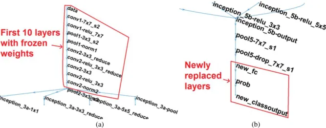
(a) (b)
Figure 1 GoogLeNet layers a) zoomed in GoogLeNet layer showing the first 10 layers whose weights are frozen before training initialization, b) zoomed in GoogLeNet layer tree showing the newly replaced layers connected in the end
3 choose among different filter sizes and sequences of layers.
Meanwhile, GoogLeNet provides the opportunity to use all the different combinations in parallel (which is known as the inception module [19]), thus improving the optimisation process. Also, GoogLeNet has previously been developed with about 1.2 million images for training so the low level features are already very rigorously learned by this model. We have taken advantage of this and build on these pre-trained low level features by only performing training of high level features specific to drone/bird classification. Even though the requirement to use an RGB dataset can be seen as disadvantageous for false colour radar image classification, this is a very well-established model to test the capability of CNN for real time drone classification.
The GoogLeNet has 144 layers in total (considering every element within the parallel inception modules as a separate layer). To reuse the pre-trained network, the weights of the first 10 layers (corresponding to low level feature learning) have been frozen by setting the learning rate values as zero for those layers, seen in Fig. 1(a). These early layers contain information on generic low-level image features (edges, curves etc.) and provide a strong foundation for learning the high-level features specific to the drone and bird dataset. We have changed the final two layers named ‘loss3-classifier’ and ‘output’. The first one is the fully connected last learnable layer and the latter one is the final classification layer. There is a ‘Softmax’ layer in between these two which designates decimal probability values for each class. The ‘loss3-classifier’ is replaced by a new fully connected layer according to the number of classes we are using for training, whereas the actual GoogLeNet model consists of a 1,000 class fully connected layer. The ‘output’ layer is then replaced with the appropriate class labels that are going to be used during training. Fig.1(b) is the zoomed in layer graph plot of the GoogLeNet model (generated in Matlab), verifying that the new layers are properly connected.
2.2. Series Network
Unlike GoogLeNet, a series network consists of layers connected serially with each other (no multiple inputs or outputs for any layer). This is a simpler model with the flexibility of easily manipulating the convolutional layer filter sizes. Hence, we have decided to create a series network to train the grayscale image dataset. We have created different variations of the model to find out the optimal version.
We have used a Stochastic Gradient Descent with Momentum (sgdm) optimiser during training, which is very widely used [22]. This used the backpropagation process to minimise the loss function by updating the weights in the opposite direction of the loss function gradient. Conventionally, the momentum value is set between 0.9 and 0.95. We used 0.9 meaning that 90% of information from the previous iteration will be used for the next iteration. Here, one iteration means processing of a single batch of images, both forward and backward.
The main aspect that was considered was to ensure the generalisation of the model (i.e. that the model did not suffer from over-fitting). Therefore, we have run the model with different learning rates and tested the performance afterwards. To overcome the over-fitting problem, a regularisation method is also often used which requires the
modification of the performance function during training. We have split the labelled dataset into training and validation data (randomly selected before the training starts). The validation dataset is used during training at specified intervals to check if the model is over-fitting or not. L2 regularisation (Ridge regression) [23] is implemented during training as well which adds a penalty term to the loss function. A small value of 1e-4 was set for this to avoid under-fitting.
Learning rate is a very important parameter which controls the change of weights during training. The model will get under-fitted and will have difficulty converging if the learning rate value is quite large whilst a very small value will make the model vulnerable to over-fitting. There is no standard learning rate value which can be generically used for all types of datasets. ImageNet, which was developed by Microsoft, used the initial learning rate value of 0.1 [24]. Decreasing the learning rate from an initially large value during training is also a common practice, as it is difficult to select the optimum value in the beginning. Our assumption is that the spectrogram image based model can be more prone to over-fitting than optical image based classification training because a physical shape of an object is more concrete than its micro-Doppler signatures. Hence, to be extra cautious, we omitted adaptive rate scheduling to enforce the model not to reduce the learning rate during training. Instead, we have trained the model with different learning rates and carefully compared the results. We have used five different values (0.0005, 0.001, 0.01, 0.1, and 0.2) during training. As can be seen, the range of values here is quite large to discover the optimum spot between under-fitting and over-under-fitting. The performance comparison is discussed in section 4.
Another factor which is important for generalisation is the dropout rate. The dropout layer randomly assigns zero to a certain number of input elements (defined by a probability value) after the first fully connected layer. The idea behind this is that by relearning multiple times, noise in the dataset will be cancelled out and the model will become more generalised. We have trained the model without dropout and with 50% dropout. The performance of the model with dropout has been found to be significantly better, which again will be shown later.
We have used different combinations of convolutional layer filter sizes. All the combinations include 5x5 and 3x3 filters, with a different number of filters in each layer. Using more filters in each layer enables better preservation of the spatial dimensions. A larger filter size of 7x7 has also been tested but did not produce better results and hence was discarded. Conventionally, every convolutional layer is followed by a ReLU (Rectified Linear Units) layer and a Maxpool layer. A ReLU layer is used to incorporate nonlinearity in the model because the convolutional layer operation is linear (multiplication between filter values and pixel values). This layer basically changes the negative values of each pixel after the convolutional layer to zero. Using this makes the training faster compared to conventional nonlinear functions (e.g. sigmoid). A Maxpool layer is then used for down-sampling the array by taking the maximum from a specified area. In this case, we have used the Maxpool layer size as 2x2 with stride [2 2]. When the same convolutional layer filter size and numbers are used on back-to-back layers (with different strides), a Maxpool layer
4 is then not used in between. The convolutional layer strides
are set as [1 1] as well as [2 2] to introduce more diversity to feature learning.
We have also implemented a batch normalisation layer between every convolutional and ReLU layer which speeds up the training. Also, as the initial weights of the network in the CNN are randomly assigned, a batch normalisation layer helps to make the model less sensitive to initialisation values. Each value is normalised by subtracting the mean of the batch during the iteration, then dividing by the standard deviation of the batch.
We have trained the model by using the convolutional network size range from 16 to 32 in the first place. Then we have increased the network by adding more convolutional layers with sizes varying from 16 to 128. This makes the model more rigorous which has been validated by the training and validation accuracy performance.
An average pooling layer before the dropout layer has been tried as well. This layer is used for down-sampling the
input by dividing it into smaller rectangular regions and then taking the average. We have found out this decreases the training accuracy hence we omitted it from the final version.
Table 1 Series Network layers
Layer Name Type Description
1 'input' Image Input 224x224x1 images with 'zerocenter' normalization 2 'conv_1' Convolution 16 5x5 convolutions with stride [1 1] and padding 'same' 3 'BN_1' Batch normalization Batch Normalization
4 'relu_1' ReLU ReLU
5 ‘Maxpool_1’ Max Pooling 2x2 max pooling with stride [2 2] and padding [0 0 0 0] 6 'conv_2' Convolution 32 5x5 convolutions with stride [1 1] and padding 'same' 7 'BN_2' Batch normalization Batch Normalization
8 'relu_2' ReLU ReLU
9 ‘Maxpool_2’ Max Pooling 2x2 max pooling with stride [2 2] and padding [0 0 0 0] 10 'conv_3' Convolution 32 3x3 convolutions with stride [2 2] and padding 'same' 11 'BN_3' Batch normalization Batch Normalization
12 'relu_3' ReLU ReLU
13 'conv_4' Convolution 32 3x3 convolutions with stride [1 1] and padding 'same' 14 'BN_4' Batch normalization Batch Normalization
15 'relu_4' ReLU ReLU
16 ‘Maxpool_3’ Max Pooling 2x2 max pooling with stride [2 2] and padding [0 0 0 0] 17 'conv_5' Convolution 64 3x3 convolutions with stride [2 2] and padding 'same' 18 'BN_5' Batch normalization Batch Normalization
19 'relu_5' ReLU ReLU
20 'conv_6' Convolution 64 3x3 convolutions with stride [1 1] and padding 'same' 21 'BN_6' Batch normalization Batch Normalization
22 'relu_6' ReLU ReLU
23 ‘Maxpool_4’ Max Pooling 2x2 max pooling with stride [2 2] and padding [0 0 0 0] 24 'conv_7' Convolution 128 3x3 convolutions with stride [2 2] and padding 'same' 25 'BN_7' Batch normalization Batch Normalization
26 'relu_7' ReLU ReLU
27 'conv_8' Convolution 128 3x3 convolutions with stride [1 1] and padding 'same' 28 'BN_8' Batch normalization Batch Normalization
29 'relu_8' ReLU ReLU
30 ‘Maxpool_5’ Max Pooling 2x2 max pooling with stride [2 2] and padding [0 0 0 0] 31 ‘dropout’ Dropout 50% dropout
32 ‘fc’ Fully connected 4 fully connected layer 33 ‘Softmax’ Softmax Softmax
34 ‘Classoutput’ Classification output Final classification output
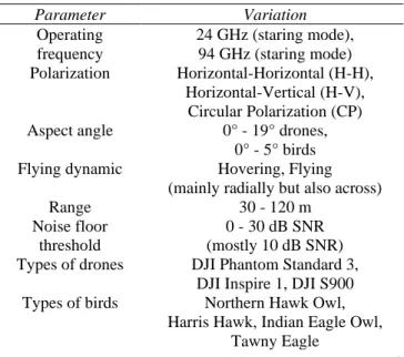
Table 2 Training dataset image diversities
Parameter Variation Operating frequency 24 GHz (staring mode), 94 GHz (staring mode) Polarization Horizontal-Horizontal (H-H), Horizontal-Vertical (H-V), Circular Polarization (CP) Aspect angle 0° - 19° drones,
0° - 5° birds Flying dynamic Hovering, Flying
(mainly radially but also across) Range 30 - 120 m
Noise floor threshold
0 - 30 dB SNR (mostly 10 dB SNR) Types of drones DJI Phantom Standard 3,
DJI Inspire 1, DJI S900 Types of birds Northern Hawk Owl,
Harris Hawk, Indian Eagle Owl, Tawny Eagle
5 The series network that we have developed which
demonstrates the best performance consists of 34 layers. Table 1 illustrates the whole network with a short description of each layer. It is seen that padding is also used so that the input and output size remain the same for stride size [1 1] and rounded values of the input size divided by stride. This ensures that the edge values of the image are not correlated less than the inner values when the filter is sliding end to end. We have trained this model with all the different learning rates mentioned earlier, for both 4-class and 2-class training.
3. Training dataset
Our aim was to ensure that the training dataset resembles images to be expected from a real time drone detection radar system. The best way to do this was to use actual in-flight micro-Doppler spectrograms obtained from experimental trials. We did this for both 4-class and 2-class training. We have obtained a large amount of in-flight drone and bird data to analyse micro-Doppler signatures at K-band and W-band [25]. We have used that extensive experimental data set to select images for all the training purposes. As the GoogLeNet image format is fixed, we have used the same size for the grayscale images as well. For GoogLeNet, the image format is RGB 224x224x3. The RGB images are produced using the Matlab colourscale ‘Jet (256)’. The grayscale image generation was slightly indirect, as the Matlab gray colourscale is also in RGB format. To create images in the desired 224x224x1 format, the corresponding matrix values have been converted to an index of 8-bit integer values and then converted to gray. This omits the hue and saturation information whilst keeping the luminance information hence making the image monochromatic.
Each spectrogram image is produced from 0.4 seconds worth of FMCW radar data. This is a trade-off between having enough micro-Doppler information within one image and classification time. Whilst we also have a large set of CW images, we have not included those in this study. This is because our intention is that the trained model can be used by a real time drone classification system which requires tracking and hence entails the use of range-Doppler FMCW radar data. We have processed around 50,000 images in total to select images for the training. For 4-class training, the labels are defined as ‘drone’, ‘bird’, ‘clutter’ and ‘noise’. Here, clutter corresponds to the surrounding static targets, appearing as the zero-Doppler values in the spectrogram (horizontal band in the middle). We have selected 600 images for each label, 2,400 images in total. For 2-class training, the labels are ‘drone’ and ‘non-drone’. 1,000 images have been selected for each label in this case, 2,000 images in total. The reason for having a smaller number of images for 4-class training is because fewer bird images were available (as it was not straight forward to keep
Table 3 Radar parameters
Parameters 94 GHz 24 GHz
Operating mode FMCW, staring FMCW, staring Chirp repetition frequency (CRF) 12.4 kHz 4.25 kHz
Maximum unambiguous velocity ±9.93 ms-1 ±13.3 ms-1
STFT length 512 samples (41.2 ms) 512 samples (120.2 ms)
STFT overlap 95% 95%
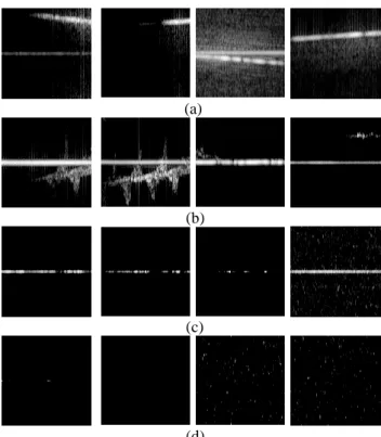
(a)
(b)
(c)
(d)
Figure 2 Example RGB training data a) drone, b) bird, c) clutter, d) noise. X-axis is time, Y-axis is velocity
(a)
(b)
(c)
(d)
Figure 3 Example grayscale training data a) drone, b) bird, c) clutter, d) noise. X-axis is time, Y-axis is velocity
6 the birds well within the antenna beam all the time). All the
images are obtained with the radars operating in staring mode. The selection of the images from the large pool was done to ensure that each label does not become homogenous. The diversity will be more apparent in the drone and bird datasets, as the scenarios there are more dynamic. Also, as mentioned before, for direct comparison between the two models, the RGB dataset and the grayscale dataset consist of exactly the same images in jet 256 and grayscale colour maps respectively. We have intentionally omitted using synthetic data augmentation to retain only authentic data for training. We have split the dataset during training in to two sections, training and validation. 80% of the images were selected for training and the remaining 20% were for validation. To be as generic as possible, the selection was done randomly by the code. The 80%-20% division has been chosen by considering various trade-offs. Usually, for a very large dataset (e.g. dataset used for original GoogLeNet training), having a good portion of the data for validation purpose is useful. This reduces the training time without considerably increasing the variance in parameter estimation so a 70%-30% or even a 60%-40% spilt can be made. In contrast, with a small dataset (e.g. ~100 images for each class), most of the data need to be used for training (i.e. 90%-10% split), otherwise the model will not get trained properly. We consider the size of our dataset to be in the middle-range. Hence, we designed the training with the 80%-20% split, which is quite commonly used. It should be noted that we have not used any images within these datasets to test the performance of the trained models afterwards. Those are done with entirely separate, unseen and unlabelled images.
Table 2 shows the various aspects that have been varied during image selection to create a diverse training set. The types of drones and birds vary in sizes and weights. It should be noted that whilst we have varied the noise floor threshold for generalisation, it should not be varied too much. As propellers are usually under-sampled in the Doppler domain for an FMCW radar, there is a
characteristic spread of micro-Doppler signatures (seen in Fig. 2). Setting the noise floor threshold too low will then create ambiguity and consequently decrease the classification performance. This means, there should be a compromise while setting the noise threshold. Too high a threshold can lose the propeller blade returns whereas too low a threshold can increase the false
alarm rate. Eventually, this is up to the training model developer to decide on, which will depend on application requirements.
Table 3 provides some of the relevant radar parameters (94 GHz radar, named T-220 [26], and 24 GHz (a) (b)
(c) (d)
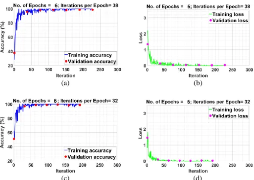
Figure 4 GoogleNet training and validation accuracy and loss function plots, a-b) for 4-class, c-d) for 2-class
(a)
(b)
Figure 5 Effect of dropout layer for series network a) with 50% dropout, b) without dropout
7 radar [27]) used for the spectrogram image processing.
Fig. 2 shows some example RGB images obtained directly from the training dataset. The vertical axis of the images corresponds to velocity (+/-), with positive velocity on the top half, negative velocity on the bottom half and zero in the middle. The horizontal axis corresponds to time. The variety of data can be seen here, especially from the drone and bird images. In Figs. 2(a), the drone is partially within the spectrogram in the first image, barely within the spectrogram in the second image and fully within the spectrogram in the last two images. In Figs. 2(b), the bird is partially within the spectrogram in the first image, fully within the spectrogram in the second image and barely within the spectrogram in the last two images, almost impossible to identify, even visually. All the corresponding grayscale images are shown in Fig. 3. It can be seen that the
signal strength of both bulk and micro-Doppler also vary in the images, depending on antenna beam coverage of the targets. This demonstrates the advantage of using real data. As both the targets fly at speeds up to 20 ms-1, the scenario
is quite dynamic. Only using spectrograms consisting of strong micro-Doppler signatures with no variation in flight dynamics would almost certainly cause the trained model to significantly underperform in real situations. Fig. 2(c) and 3(c) are examples of ground clutter whilst Figs. 2(d) and 3(d) are examples of noise.
4. Training results
The training was performed on a single quadcore CPU with 8 GB RAM. On average, the time taken for training was around 36-45 minutes for every single run. (a)
(b)
(c)
Figure 6 Training and validation accuracies of the 34 layer series network for different learning rates a) 2-class training with learning rates 0.2, 0.1, 0.01, 0.001 and 0.0005 respectively, b) Example of model overfitting and degraded accuracy without validation dataset used during training (learning rate 0.0005), c) 4-class training with learning rates 0.2, 0.1, 0.01, 0.001 and 0.0005 respectively
8 Fig. 4 shows the GoogLeNet training results by
presenting the plots for accuracy and loss. The dataset has been divided into 32 batches during training hence there are 32 iterations for each Epoch for 2-class training and 38 for
4-class training. For the GoogLeNet model training, 6 Epochs have been used. The Epoch number was eventually set by running the model a few times to see when the model converged. The training should not be run significantly (a) (b)
(c) (d)
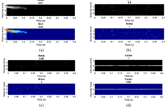
Figure 7 Example classification performance figures comparing series network (grayscale) and GoogLeNet (RGB) using test dataset where the title of each image is the target classified by the network and below that is the confidence level with maximum value of 1, showing: a) both networks accurately classifying a drone, b) series network missing a drone, c) both networks accurately classifying a bird, d) both network accurately classifying a bird even when the bird is not entirely within the image
(a) (b)
(c) (d)
Figure 8 More example classification performance figures comparing series network (grayscale) and GoogLeNet (RGB) using test dataset where the title of each image is the target classified by the network and below that is the confidence level with maximum value of 1, showing: a) series network wrongly identifying a bird as a drone, b) series network wrongly identifying noise as a bird, c) both networks correctly identifying noise, d) both networks correctly identifying clutter
9 longer once the plots saturate as then the model might start
to learn noise. The learning rate was set to 0.001 in this case. We have also trained with other values and found this gives the best validation accuracy. The validation frequency was set to 32 iterations. As seen in Fig. 4, validation and training accuracy remain very close - a very good indication of the model generalisation. The training accuracy in both cases reaches 100% and the validation accuracy is 99.1% for 2-class network and 99.0% for 4-2-class network. This demonstrates the strength of GoogLeNet for discriminating drones from birds and clutter.
For the series network training, different variations have been used before obtaining the optimum model. Fig. 5 shows the effect of dropout. Here the training was performed both with and without the dropout layer activated in the series network shown in Table 1. It is seen that the validation accuracy for the 4-class network is 95.9% with dropout but 91.3% without dropout. In each case, the training accuracy is ~100%. This suggests that the model has been over-fitted. Also, not using dropout makes the performance worse.
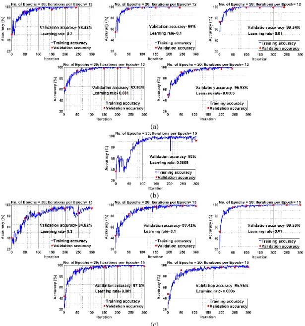
Fig. 6 shows the training and validation performances of the 34 layer series network in Table 1 for different learning rates and for both 4-class and 2-class networks. The number of Epochs was set to 20 eventually in this case after testing with a few different values. The number of iterations per Epoch is 12 for the 2-class network and 15 for the 4-class network. The validation frequency is set to 50. Not using the validation data during training again makes the model more prone to over-fitting as it cannot check for that during training and hence cannot modify the weights accordingly if needed. An example of this is provided in Fig. 6(b) where the validation is performed only after the training has ended, giving poorer performance. It has been found that the best performance is achieved with the learning rate being 0.01, where the validation accuracies are more than 99% in both cases. Values smaller or greater
show the trend of the validation accuracy gradually decreasing.
5. Test results
After the whole training process was completed, we tested the models with entirely unseen and unlabelled datasets. We ran various datasets with flying drones or birds and let the models classify on the fly. We then manually verified whether correct prediction had been made. Subsequently, we quantified the prediction accuracy percentage. We have found that most of the time the accuracy with the test dataset is slightly lower than the validation accuracy but is still quite high. Initially, we ran a 94 GHz data file in which a DJI Inspire 1 is flying from 70-80 m range. A total of 556 spectrogram plots were generated covering this range. It should be noted that this test dataset includes noise and clutter along with drone micro-Doppler as the drone is moving and hence changing range bins. As it is extremely time consuming to manually check for all the models with different learning rates and different number of classes, we have used only the model which performed best during training (with 0.01 learning rate value). Similar manual verification has also been performed with bird data. The bird (Harris Hawk) flew from 30-100 m although it was out of the beam most of the time as the flight path was not straight. We thus chose a range of 70-100 m yielding 746 images with a good combination of bird and non-bird spectrograms.
Fig. 7 and Fig. 8 show example figures of with prediction results from the two classification methods using the test data. The spectrograms are generated simultaneously and the direct comparison between the GoogLeNet and the series network can be visually observed. The performances have been visually verified and then recorded.
The overall test prediction accuracy is given in Table 4 which shows that GoogLeNet outperforms the series (a) (b)
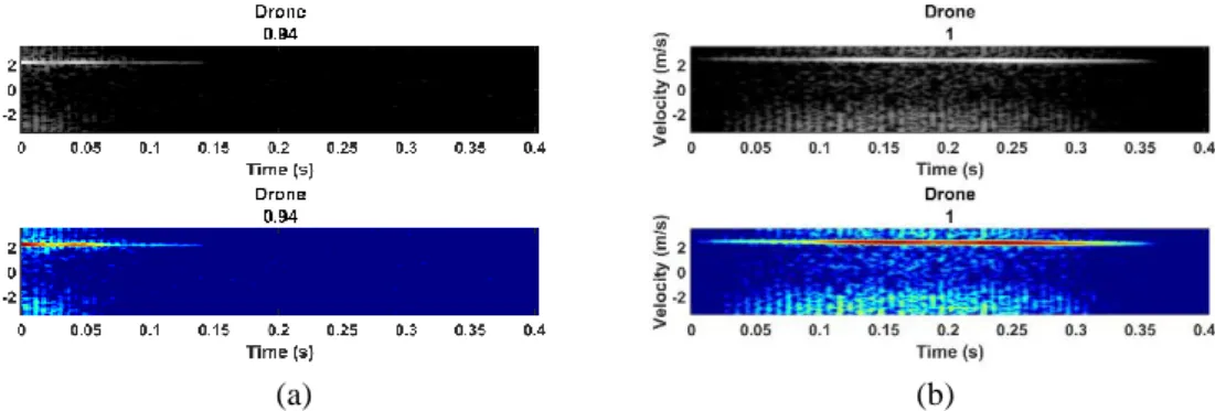
Figure 9 Example classification performance figures for NIRAD data which was never used during training where the title of each image is the target classified by the network and below that is the confidence level with maximum value of 1, showing a-b) both networks correctly classifying the drone
Table 4 Test data prediction accuracy
Test drone data file Test bird data file
Number of spectrograms 556 746
Series network accuracy (4-class) 525 (94.42%) 728 (97.59%) GoogLeNet accuracy (4-class) 549 (98.74%) 741 (99.32%) Series network accuracy (2class) 546 (98.20%) 732 (98.12%) GoogLeNet accuracy (2-class) 553 (99.46%) 746 (100%)
10 network in all cases. This suggests that the series network is
not entirely immune to over-fitting. Nonetheless, it should be stressed that we have pushed the classification model to its limit and have obtained test accuracies well over 90% in all cases.
We have also tested the false alarm rate by selecting 324 images from the test bird data where every image fully or partially consists of bird micro-Doppler. We then ran the 2-class network and checked the number of times the image is predicted as drone. The series network predicted 4 images as drone, giving a false alarm rate of 1.23%. In contrast, GoogLeNet did not label a single image as drone providing a 0% false alarm rate. In a real time surveillance application, a 1.23% false alarm rate may be higher than desired, but this is the raw individual image false alarm rate. The alert system of the classifier can be set to alarm only with successive hits (e.g. 2 or 3 images in a row being predicted as drone) which would decrease the false alarm rate to a suitable level.
Finally, we have also tested the prediction performance by using data from an entirely different W-band FMCW radar, named NIRAD [28]. This was done to verify the generalisation of the trained models. A data file was chosen where the drone was flying from 75-80 m range (no bird data was available with this radar) and 204 spectrograms were generated. Fig. 9 shows couple of example figures of the classification performance of NIRAD data. The accuracy was 95.1% for 4-class series network, 98.5% for 2-class series network, 98.5% for 4-class GoogLeNet and 99.0% for 2-class GoogLeNet. This illustrates that the developed models have sufficient performance to be integrated into a real time radar based drone detection system.
It can be argued that the GoogLeNet should be used in all cases as it offers better performance than the series network. However, there are two factors that go in favour of the series network. One is the colourscale issue with the GoogLeNet as it remains to be seen if any random colourscale performs equally well compared to others all the time. The second factor is the computational time during classification. When a single image is fed to the trained model, the average time taken by the GoogLeNet is 0.4 seconds whilst the average time taken by the series network is 0.05 seconds, i.e. eight times faster. This is understandable as GoogLeNet is a large network compared to the series network. Also, the convolutional layer filters are applied to a single dimension in the case of the series network whereas they are applied to three dimensions in case of 224x224x3 RGB images in GoogLeNet. This contributes to the faster classification time for the series network. For a real-time application in which a drone can move at 10-20 ms-1, the faster classification time gives the
series network a significant advantage.
6. Conclusion
In this study, we have successfully created a neural network training dataset for drone classification using only experimental data obtained in dynamic scenarios. Both a pre-trained model (GoogLeNet) and our own developed series network have been used for training and both have shown well above 90% accuracy. Both models have been tested with previously unseen data and have again shown
very good accuracy. GoogLeNet performs better but is more time consuming compared to the series network. It has been shown that they can be used in practical scenarios.
The obvious potential of the CNN classifiers demonstrated here suggests that, via further optimisation, they can be used to achieve an extremely robust radar sensor based classification system. We anticipate that this approach can be translated in to other types of target classification algorithm development using spectrogram images (i.e. various human activities, different types of animals etc.). The best way to improve a CNN model is to make the dataset larger and more diverse. The continuation of this work is then to include more drone and bird data, particularly including a wider diversity of different clutter surroundings. Additionally, more complex images consisting of two birds in a single spectrogram or a bird and a drone in one image can be trained. This extra complexity will be more challenging to the CNN model hence might require further refinement of the current model. It will also be interesting to quantitively compare the classification performance we achieved here with other algorithms. A proper comparison can only be made if they are tested under the same scenario (i.e. with the same dataset). We realize that the large dataset that we have created can be of great value to other researchers developing different classification models. Therefore, we would be happy to share the data on request. We hope this would benefit the ongoing effort within the field to develop a robust, real-time drone detection algorithm, which can be broadly used by diverse types of radar systems.
7. Acknowledgments
The authors acknowledge the funding received from the Science and Technology Facilities Council which has supported this work under grant ST/N006569/1. The authors also acknowledge the contribution of ‘Elite Falconry’ for the bird data collection and Dr Rob Hunter, Dr Adeola Fabola and Dr Paddy Pomeroy for flying the drones.
8. References
[1] I. Guvenc, F. Koohifar, S. Singh, M. L. Sichitiu, and D. Matolak, “Detection, Tracking, and Interdiction for Amateur Drones,” IEEE Commun. Mag., vol. 56, no. 4, pp. 75–81, Apr. 2018.
[2] J. S. Patel, F. Fioranelli, and D. Anderson, “Review of radar classification and RCS characterisation techniques for small UAVs ordrones,” IET Radar, Sonar Navig., vol. 12, no. 9, pp. 911–919, Sep. 2018. [3] V. C. Chen, The micro-doppler effect in radar.
Artech House, 2011.
[4] S. Rahman and D. A. Robertson, “Millimeter-wave micro-Doppler measurements of small UAVs,” in
Proc. SPIE 10188, Radar Sensor Technology XXI, 2017, vol. 10188, p. 101880T.
[5] J. de Wit, “Micro-Doppler analysis of small UAVs,”
in 2012 9th European Radar Conference : 31
October - 2 November 2012, Amsterdam, the Netherlands, 2012, pp. 210–213.
[6] P. Molchanov, R. I. A. Harmanny, J. J. M. de Wit, K. Egiazarian, and J. Astola, “Classification of small UAVs and birds by micro-Doppler signatures,” Int. J. Microw. Wirel. Technol., vol. 6, no. 3–4, pp. 435–
11 444, 2014.
[7] M. Ritchie, F. Fioranelli, H. Borrion, and H. Griffiths, “Classification of loaded/unloaded micro-drones using multistatic radar,” Electron. Lett., vol. 51, no. 22, pp. 1813–1815, Oct. 2015.
[8] M. Ritchie, F. Fioranelli, H. Griffiths, and B. Torvik, “Monostatic and bistatic radar measurements of birds and micro-drone,” in 2016 IEEE Radar Conference (RadarConf), 2016, pp. 1–5.
[9] L. Fuhrmann, O. Biallawons, J. Klare, R. Panhuber, R. Klenke, and J. Ender, “Micro-Doppler analysis and classification of UAVs at Ka band,” in 2017 18th International Radar Symposium (IRS), 2017, pp. 1–9.
[10] Y. Kim and T. Moon, “Human Detection and Activity Classification Based on Micro-Doppler Signatures Using Deep Convolutional Neural Networks,” IEEE Geosci. Remote Sens. Lett., vol. 13, no. 1, pp. 8–12, Jan. 2016.
[11] A. Angelov, A. Robertson, R. Murray-Smith, and F. Fioranelli, “Practical classification of different moving targets using automotive radar and deep neural networks,” IET Radar, Sonar Navig., vol. 12, no. 10, pp. 1082–1089, Oct. 2018.
[12] J. S. Patel, F. Fioranelli, M. Ritchie, and H. Griffiths, “Multistatic radar classification of armed vs unarmed personnel using neural networks,” Evol. Syst., vol. 9, no. 2, pp. 135–144, Jun. 2018.
[13] Z. Chen, G. Li, F. Fioranelli, and H. Griffiths, “Personnel Recognition and Gait Classification Based on Multistatic Micro-Doppler Signatures Using Deep Convolutional Neural Networks,” IEEE Geosci. Remote Sens. Lett., vol. 15, no. 5, pp. 669– 673, May 2018.
[14] A. Schumann, L. Sommer, J. Klatte, T. Schuchert, and J. Beyerer, “Deep cross-domain flying object classification for robust UAV detection,” in 2017 14th IEEE International Conference on Advanced
Video and Signal Based Surveillance (AVSS), 2017,
pp. 1–6.
[15] “Drone-vs-Bird Detection Challenge – International Workshop on Small-Drone Surveillance, Detection and Counteraction Techniques.” [Online]. Available: https://wosdetc.wordpress.com/challenge/.
[Accessed: 07-Jul-2019].
[16] D. A. Brooks, O. Schwander, F. Barbaresco, J.-Y. Schneider, and M. Cord, “Temporal Deep Learning for Drone Micro-Doppler Classification,” in 2018 19th International Radar Symposium (IRS), 2018, pp. 1–10.
[17] D. Choi, Byunggil: Oh, “Classification of Drone Type Using Deep Convolutional Neural Networks Based on Micro- Doppler Simulation,” in ISAP 2018 : 2018 International Symposium on Antennas and Propagation : October 23-26, 2018, Paradise Hotel Busan, Busan, Korea, 2018.
[18] B. K. Kim, H.-S. Kang, and S.-O. Park, “Drone Classification Using Convolutional Neural Networks With Merged Doppler Images,” IEEE Geosci. Remote Sens. Lett., vol. 14, no. 1, pp. 38–42, Jan. 2017.
[19] C. Szegedy et al., “Going deeper with convolutions,”
in 2015 IEEE Conference on Computer Vision and
Pattern Recognition (CVPR), 2015, pp. 1–9.
[20] M. S. Seyfioglu and S. Z. Gurbuz, “Deep Neural Network Initialization Methods for Micro-Doppler Classification With Low Training Sample Support,”
IEEE Geosci. Remote Sens. Lett., vol. 14, no. 12, pp. 2462–2466, Dec. 2017.
[21] S. S. Haykin, Neural networks : a comprehensive
foundation. Prentice Hall, 1999.
[22] D. P. Kingma and J. Ba, “Adam: A Method for Stochastic Optimization,” Dec. 2014.
[23] A. E. Hoerl and R. W. Kennard, “Ridge Regression: Biased Estimation for Nonorthogonal Problems,”
Technometrics, vol. 12, no. 1, pp. 55–67, Feb. 1970. [24] K. He, X. Zhang, S. Ren, and J. Sun, “Deep
Residual Learning for Image Recognition,” in 2016 IEEE Conference on Computer Vision and Pattern
Recognition (CVPR), 2016, pp. 770–778.
[25] S. Rahman and D. A. Robertson, “Radar micro-Doppler signatures of drones and birds at K-band and W-band,” Sci. Rep., vol. 8, no. 1, p. 17396, Dec. 2018.
[26] D. A. Robertson, G. M. Brooker, and P. D. L. Beasley, “Very low-phase noise, coherent 94GHz radar for micro-Doppler and vibrometry studies,” in
Proc. SPIE 9077, Radar Sensor Technology XVIII, 2014, vol. 9077, p. 907719.
[27] S. Rahman and D. A. Robertson, “Coherent 24 GHz FMCW radar system for micro-Doppler studies,” in
Radar Sensor Technology XXII, 2018, vol. 10633, p. 17.
[28] D. A. Robertson and S. L. Cassidy, “Micro-doppler and vibrometry at millimeter and sub-millimeter wavelengths,” in Proc. SPIE 8714, Radar Sensor Technology XVII, 2013, vol. 8714, p. 87141C.