Keeping the balance—Bridge sampling for marginal likelihood estimation in finite mixture, mixture of experts and Markov mixture models

(1)

ePub

Institutional Repository

Sylvia Frühwirth-Schnatter

Keeping the balance—Bridge sampling for marginal likelihood estimation in

finite mixture, mixture of experts and Markov mixture models

Article (Published) (Refereed)

Original Citation:

Frühwirth-Schnatter, Sylvia (2019)

Keeping the balance—Bridge sampling for marginal likelihood estimation in finite mixture, mixture of experts and Markov mixture models.

Brazilian Journal of Probability and Statistics, 33 (4). pp. 706-733. ISSN 0103-0752

This version is available at: https://epub.wu.ac.at/7730/ Available in ePubWU: September 2020

ePubWU_{, the institutional repository of the WU Vienna University of Economics and Business, is}

provided by the University Library and the IT-Services. The aim is to enable open access to the scholarly output of the WU.

This document is the publisher-created published version.

(2)

2019, Vol. 33, No. 4, 706–733 https://doi.org/10.1214/19-BJPS446 ©Brazilian Statistical Association, 2019

Keeping the balance—Bridge sampling for marginal

likelihood estimation in finite mixture, mixture of experts

and Markov mixture models

Sylvia Frühwirth-Schnatter

Vienna University of Economics and Business (WU), Austria Abstract. Finite mixture models and their extensions to Markov mixture and mixture of experts models are very popular in analysing data of various kind. A challenge for these models is choosing the number of components based on marginal likelihoods. The present paper suggests two innovative, generic bridge sampling estimators of the marginal likelihood that are based on con-structing balanced importance densities from the conditional densities arising during Gibbs sampling. The full permutation bridge sampling estimator is de-rived from considering all possible permutations of the mixture labels for a subset of these densities. For the double random permutation bridge sampling estimator, two levels of random permutations are applied, first to permute the labels of the MCMC draws and second to randomly permute the labels of the conditional densities arising during Gibbs sampling. Various applications show very good performance of these estimators in comparison to importance and to reciprocal importance sampling estimators derived from the same im-portance densities.

1 Introduction

Finite mixture models and their extensions to Markov mixture and mixture of ex-perts models are very popular in analysing data of various kind. These models are useful for flexible modelling, density estimation and unsupervised clustering, see, for example,Frühwirth-Schnatter(2006) andFrühwirth-Schnatter, Celeux and Robert(2019) for a recent review. The various types of mixture models share a common structure insofar as it is supposed that N observationsy=(y1, . . . ,yN)

are generated by K hidden groups/states. If the unknown group/state indicators

S=(S1, . . . , SN)are introduced as missing data, then the different model classes

differ in their assumption concerning the distribution of the latent indicatorsS. For a finite mixture model, the indicatorsSi are i.i.d. with Pr(Si=k)=ηkand

a mixture with weight distribution η=(η1, . . . , ηK)results as marginal

distribu-tion ofyi. For a mixture of experts model, the indicators Si are still independent,

but the weight distribution Pr(Si=k|xi)depends on covariatesxi and additional

parametersγ. For Markov mixture models,y=(y1, . . . ,yN)is a time series and

Key words and phrases.Markov chain Monte Carlo, model-based clustering, Gaussian mixtures, hierarchical priors, permutation sampling, importance sampling.

Received February 2019; accepted April 2019.

(3)

Si is a hidden Markov chain with transition matrixξ. Given the group indicator

Si, for all three model classes yi|Si=k arises from a distributionp(yi|θk) with

group-specific parameterθkthat might also depend on covariates.

A challenge for any kind of mixture model is choosing the numberK of hidden states/groups, see Celeux, Frühwirth-Schnatter and Robert(2019) for a compre-hensive review. For finite mixtures, reversible jump MCMC methods (Richardson and Green, 1997) have been employed to sample from the posterior p(K|y), however these methods are very challenging to implement. An attractive alter-native to choose the number of hidden groups in a model-based clustering con-text are sparse finite mixture models (Malsiner Walli, Frühwirth-Schnatter and Grün, 2016). However, this approach does not allow comparisons across differ-ent model classes or differdiffer-ent prior choices and so far has not been extended to hidden Markov and Markov switching models. A very general form of model se-lection can be achieved by comparing models and priors through marginal likeli-hoods and reliable estimators of the marginal likelihood are important for Bayesian model selection

Hence, in the present paper, we focus on Bayesian model choice among mixture models of increasing number of components K through the marginal likelihood

p(y|K), defined as

p(y|K)=

p(y|ϑ, K)p(ϑ|K)dϑ. (1) In (1),ϑ=(θ1, . . . ,θK,ω)summarizes all unknown parameters, withωbeing a

generic notation for the parameters in the weight distribution for all three types of mixture models considered in this paper. The marginal likelihood naturally pe-nalises models with more mixture components (and more parameters), see, for example,Berger and Jefferys(1992); however, for mixture models it is not avail-able in closed form and computational approximation methods become an integral part of model selection.

Frühwirth-Schnatter (2004) introduced simulation-based estimators such as importance sampling (Geweke, 1989), reciprocal importance sampling (Gelfand and Dey, 1994) or bridge sampling (Meng and Wong, 1996) to approximate the marginal likelihood for finite mixture and Markov switching models with moder-ate values ofK. For such sampling-based techniques, one has to select for eachK

an importance densityqK(ϑ)which is easy to sample from and provides a rough

approximation to the mixture posterior density p(ϑ|y, K). However, for mixture models, it is not at all straightforward to choose an appropriate importance density and the reliability of the resulting sampling-based estimators depends on several factors.

First, as shown by Frühwirth-Schnatter (2004), the tail behaviour of the im-portance density qK(ϑ) compared to the mixture posterior p(ϑ|y, K) matters.

Whereas the (optimal) bridge sampling estimator (which will be reviewed in Sec-tion2) is fairly robust in this respect, other sampling-based estimators are more

(4)

sensitive. For instance, importance sampling which is based on rewriting (1) as

p(y|K)=

_p(y_|_ϑ_{, K)p(}_ϑ_|_K) qK(ϑ)

qK(ϑ)dϑ, (2)

exhibits high standard errors, ifqK(ϑ)has thin tails compared to the mixture

pos-teriorp(ϑ|y, K).

Second, as pointed out byLee and Robert(2016), the importance densityqK(ϑ)

has to mimic the multimodality of the mixture posteriorp(ϑ|y, K)which is caused by the invariance of a mixture model with symmetric priors for the components to permutations of the mixture component labels, the so-called label switching prob-lem. As proven inRousseau, Grazian and Lee(2019), the number of symmetric modes in the posterior distribution p(ϑ|y, K) tends to K! as the number of ob-servations N increases. A balanced importance density covers all modes of the posterior or, more formally,qK(ϑ)is (nearly) invariant to permuting the labels of

ϑ. If the importance density is unbalanced and several modes of the mixture pos-terior are not covered, then sampling-based estimators of the marginal likelihood are prone to be biased.

Several approaches have been suggested to ensure multimodality in the con-struction of the importance density also for increasing values of K. Frühwirth-Schnatter (2004) constructs the importance density from the output of random permutation posterior sampling (Frühwirth-Schnatter, 2001). However, as demon-strated inCeleux, Frühwirth-Schnatter and Robert(2019) for univariate Gaussian mixtures, the resulting bridge sampling estimator might be biased, despite its ro-bustness to the tail behaviour. A first contribution of the present paper is to show that marginal likelihood estimators based on random permutation posterior sam-pling can be improved considerably by introducing a second level of random per-mutation during the construction of the importance density from the conditional densities arising during Gibbs sampling. This restores balance and yields the so-called double random permutation bridge sampling estimator.

An alternative approach is based on constructing perfectly balanced importance densities by considering all possible permutations of the labels, see, for exam-ple, Berkhof, van Mechelen and Gelman (2003) and Lee et al. (2009). Lee and Robert(2016) combine importance sampling with such a perfectly balanced im-portance density, calling the resulting estimatordual importance sampling.Celeux, Frühwirth-Schnatter and Robert(2019) show that a particularly stable estimator of the marginal likelihood, called full permutation bridge sampling estimator, is ob-tained for univariate Gaussian mixtures by combining (optimal) bridge sampling with a perfectly balanced importance densityqK(ϑ).

The main contribution of the present paper is to introduce such a full permuta-tion bridge sampling estimator of the marginal likelihood for a much broader class of mixture models, including finite mixture models of many kinds, mixture of ex-perts models as well as hidden Markov and Markov switching models. For each of

(5)

these model classes, we discuss in detail how to construct fully balanced impor-tance densities. The various estimators are illustrated and compared for the various model classes for well-known data sets. We show that for all model classes consid-ered very stable estimators of the marginal likelihood are obtained by combining (optimal) bridge sampling with a perfectly balanced importance density. On the other hand, dual importance sampling (Lee and Robert, 2016) exhibits larger stan-dard errors than double random permutation and full permutation bridge sampling estimators in many cases, in particular for overfitting mixtures.

The rest of the paper is organized as follows. Section 2 reviews bridge sam-pling estimators and discusses the construction of the importance density from the outcome of Markov chain Monte Carlo sampling. To achieve balance in the im-portance density, Section3introduces double random and full permutation bridge sampling. The implementation of these estimators for finite mixtures, Markov mix-tures and Markov switching models as well as mixture of experts models is out-lined in Section4and illustrative applications are provided in Section5. Section6 concludes.

2 Bridge sampling approximations to the marginal likelihood 2.1 Bridge sampling estimators

Meng and Wong(1996) introduced a very general bridge sampling technique to es-timate the marginal likelihood as the normalising constant of the non-normalized posterior p(y|ϑ, K)p(ϑ|K), derived from Bayes’ theorem. LetqK(ϑ) be an

ap-proximation to the posteriorp(ϑ|y, K) and let α(ϑ)be a positive function such thatα(ϑ)qK(ϑ)p(ϑ|y, K)dϑ>0. Exploiting that

α(ϑ)qK(ϑ)p(ϑ|y, K)dϑ=

α(ϑ)p(y|ϑ, K)p(ϑ|K)

p(y|K) qK(ϑ)dϑ,

yields the general bridge sampling estimator of the marginal likelihood:

p(y|K)=EqK(ϑ)(α(ϑ)p(y|ϑ, K)p(ϑ|K))

Ep(ϑ|y,K)(α(ϑ)qK(ϑ))

,

provided that all expectations are well-defined.

Meng and Wong (1996) derived an optimal choice for α(ϑ) which yields a bridge sampling estimator that requires i.i.d. draws ϑ(l), l=1, . . . , L from the importance density qK(ϑ) and i.i.d. draws from the posterior p(ϑ|y, K). As

Markov chain Monte Carlo (MCMC) draws ϑ(m), m=1, . . . , M from the pos-teriorp(ϑ|y, K) are typically autocorrelated,Meng and Schilling(1996) defined an alternative optimal bridge sampling estimator pBS(y|K) based on following functionα(ϑ):

α(ϑ)=1/L·qK(ϑ)+M·p(ϑ|y, K)

.

(6)

M is the effective sample size, estimated as Mˆ = min(M, M/ρ)ˆ , where ˆ

ρ is an estimator of the inefficiency factor of the posterior draws f(m) = p(y|ϑ(m), K)p(ϑ(m)|K). This definition ofα(ϑ)requires knowledge of the (un-known) normalizing constantp(y|K)to evaluate p(ϑ|y, K). Using the estimator

ˆ

pIS(y|K) (to be defined in (4)) as a starting value for pBSˆ ,0(y|K), the following

recursion is applied until convergence to estimate the (optimal) bridge sampling estimatorpBS(yˆ |K)=limt→∞pBSˆ ,t(y|K):

Alternative estimators are obtained by other choices ofα(ϑ), for example, choos-ing α(ϑ)=1/qK(ϑ) yields importance sampling as in (2). Based solely on the

sampleϑ(l), l=1, . . . , Lfrom the importance densityqK(ϑ), the importance

sam-pling estimator of the marginal likelihood is given by:

ˆ pIS(y|K)= 1 L L l=1 p(y|ϑ(l), K)p(ϑ(l)|K) qK(ϑ(l)) . (4)

Choosing, instead, α(ϑ)=1/(p(y|ϑ, K)p(ϑ|K)) yields the reciprocal impor-tance sampling estimator (Gelfand and Dey, 1994):

pRI(y|K)= Ep(ϑ|y,K) _q K(ϑ) p(y|ϑ, K)p(ϑ|K) ₋₁ .

This yields an estimator of the marginal likelihood solely based on the MCMC drawsϑ(m), m=1, . . . , Mfrom the posterior distributionp(ϑ|y, K):

ˆ pRI(y|K)= 1 M M m=1 qK(ϑ(m)) p(y|ϑ(m), K)p(ϑ(m)|K) ₋1 . (5)

2.2 Defining importance densities for mixture analysis

Each of the estimators introduced in the previous section requires the choice of an importance densityqK(ϑ)for increasing K. As manual tuning of the

impor-tance density for each model under consideration is rather tedious, methods for choosing sensible importance densities in an unsupervised manner have been in-troduced.DiCiccio et al.(1997), for instance, suggested various methods to con-struct Gaussian importance densities from the MCMC output. However, the mul-timodality of the posterior density of a mixture model evidently forbids such a simple choice. Frühwirth-Schnatter (1995) is an early reference using Rao– Blackwellisation (Robert and Casella, 1999) to construct the importance density in an unsupervised manner from the MCMC output. She applied this idea to marginal

(7)

likelihood estimation for linear Gaussian state space models and extended this idea to finite mixture and Markov switching models inFrühwirth-Schnatter(2004).

For mixture models, a Rao–Blackwellised approximation of the posterior dis-tribution ofϑ based on introducing the latent allocationsSas missing data yields:

p(ϑ|y, K)= p(ϑ|S,y, K)p(S|y, K)dS≈ 1 M M m=1 pϑ|S(m),y, K, (6)

where S(m), m=1, . . . , M are M posterior draws of the latent allocations S. The right-hand side of (6) is a mixture approximation of the posterior density

p(ϑ|y, K) where the component densities p(ϑ|S(m),y, K) arise in Gibbs sam-pling for mixture models (Diebolt and Robert, 1994), sinceϑ(m+1)is drawn from

p(ϑ|S(m),y, K). If this conditional density arises from a well-known family of probability distributions, then its moments are available as a by-product of Gibbs sampling and can be stored easily, making the construction of an importance den-sity based on the mixture approximation (6) fully automatic.

However, for mixture models there are several challenges with using (6) as im-portance density in bridge sampling techniques. First of all, the imim-portance density

qK(ϑ) has to mimic the multimodality of the posterior p(ϑ|y, K)which results

from invariance to label switching. Gibbs sampling might lead to (implicit) la-bel switching in S(m), meaning that the component densities p(ϑ|S(m),y, K) in (6) will cover several posterior modes. However, even ifM is very large, the re-sulting importance density qK(ϑ) very likely is unbalanced, as (6) hardly ever

coversallposterior modes equally well, if it is based on standard Gibbs sampling of (S,ϑ)(m), m=1, . . . , M. As noted earlier, balance of the importance density across all modes is important for obtaining reliable estimators for the marginal likelihood. Section3discusses various strategies to ensure that importance densi-ties for mixture models are (nearly) balanced.

Second, despite introducing the latent statesSas missing data, the conditional posteriorp(ϑ|S,y, K)is not available in closed form for many interesting mixture models. As will be shown in Section4, a mixture approximation in the spirit of (6) can be constructed for these mixture models nevertheless, taking the form

qK(ϑ)= 1 M M m=1 qK ω|˜S(m)qK θ1, . . . ,θK|˜S(m),y . (7)

In (7),S˜(m)is a generic notation summarizing all information needed to construct the mth component densitiesqK(ω|˜S(m)) andqK(θ1, . . . ,θK|˜S(m),y)at the mth

sweep of MCMC sampling. For instance, for non-Gaussian mixtures often a sec-ond level of data augmentation with latent variables z is introduced such that

p(θk|˜S(m),y) with S˜(m) =(S(m),z(m)) is of closed form. If S˜(m) =S(m), then

qK(ω|˜S(m)) = p(ω|S(m)) and qK(θ1, . . . ,θK|˜S(m),y) = p(θ1, . . . ,θK|S(m),y)

(8)

Provided balanced mixing across the posterior modes, (6) converges at a para-metric speed toward the posteriorp(ϑ|y, K)asM increases (Gelfand and Smith, 1990), whereas the density qK(ϑ) defined in (7) remains an approximation to

p(ϑ|y, K), even if M goes to infinity, unless S˜(m)=S(m). As choosing a large value ofM makes the evaluation of qK(ϑ)more expensive, an issue will be how

to constructqK(ϑ)from a subset ofQ < M component densitiesqK(ϑ|˜S(q),y)=

qK(ω|˜S(q))qK(θ1, . . . ,θK|˜S(q),y)in an efficient manner. On one hand,Qshould

be small for computational reasons, becauseqK(ϑ)has to be evaluated for each

of the Q components numerous times, for example,L times for the importance sampling estimator (4). On the other hand, to cover all symmetric modes of the posterior, a dramatically increasing value of Qproportional to K!is required as

Kincreases. Hence, estimators based on such an importance density are limited to fairly moderate values ofK, say up toK=7.

3 Achieving balance in the importance density

As discussed above, it is essential to construct the component densitiesqK(ω|˜S(m))

andqK(θ1, . . . ,θK|˜S(m),y)in (7) from MCMC sampling such thatqK(ϑ)is nearly

or even perfectly balanced. A perfectly balanced importance densityqK(ϑ)is

en-tirely invariant to relabelling the components inϑ. An efficient way to introduce multimodality inqK(ϑ)and ensure (near) balance is to force label switching in a

controlled manner.

3.1 Simple random and double random permutation estimators

An early suggestion to ensure multimodality in the construction of the importance density is based on random permutation posterior sampling (Frühwirth-Schnatter, 2004). A randomly selected permutation is applied at each sweep of MCMC sam-pling (Frühwirth-Schnatter, 2001) which creates explicit label switching in the component densitiesp(ϑ|S(m),y, K)or, more generally,qK(ϑ|˜S(m),y). A subset

of these densities of sizeQ < M is then used to construct the importance density

q_KR(ϑ)as a mixture approximation as in (7) and to compute the simple random per-mutation bridge sampling estimatorpBSˆ ,R(y|K); see Algorithm1for details.

Sim-ple random permutation sampling has been applied inFrühwirth-Schnatter(2004) to finite mixture and Markov mixture models, and has been extended to mixtures of experts models inFrühwirth-Schnatter(2011).

Random permutation posterior sampling enhances mixing over all symmetric posterior modes and guarantees multimodality of the importance density q_KR(ϑ)

defined in (8). For regular cases, the number of modes in the posterior distribu-tionp(ϑ|y, K)tends toK! as the number of observationsN increases (Rousseau, Grazian and Lee, 2019). ChoosingQ=K!M0 ensures that on average each mode

(9)

Algorithm 1Simple random permutation bridge sampling estimators

(a) Perform random permutation posterior sampling: for eachm=1, . . . , M, con-clude the mth sampling step by randomly drawing a permutation τm from

SK, the set of the K! permutations of the labels {1, . . . , K}, and

relabel-ing the mixture components: (θ(m)₁ , . . . ,θ_K(m), S₁(m), . . . , S_N(m)) is substituted by (θ(m)_τ m(1), . . . ,θ (m) τm(K), τ −1 m (S (m) 1 ), . . . , τm−1(S (m)

N )) and the parameters of the

weight distribution are relabeled accordingly. For a finite mixture model, for instance,(η₁(m), . . . , η(m)_K )is substituted by(η_τ(m)

m(1), . . . , η

(m) τm(K)).

(b) Draw (without replacement) component densities

qK(ω|˜S(q))qK(θ1, . . . ,θK|˜S(q),y) for q = 1, . . . , Q from the M

compo-nent densities qK(ϑ|˜S(m),y) derived from posterior sampling and construct

following importance density:

q_KR(ϑ)= 1 Q Q q=1 qK ω|˜S(q)qK θ1, . . . ,θK|˜S(q),y . (8)

(c) Use the importance densityq_KR(ϑ)to define the simple random permutation bridge sampling estimatorpˆBS,R(y|K)from (3).

each posterior mode. Hence, for regular cases,q_KR(ϑ)is (nearly) balanced for large enough values ofM0.

However, for less regular cases such as overfitting mixture models or small data sets, where more or less than K! posterior modes are likely to be present, the importance densityq_KR(ϑ)tends to be unbalanced even for large values ofQ. Whereas a perfectly balanced importance density is invariant to label switching (or a lack of it) in the MCMC drawsϑ(m), an imbalanced importance density can be quite sensitive in this respect. In addition, any lack of balance is amplified whenK

is large and QapproachesM, as the permutations underlying the MCMC draws are strongly tied to the permutations underlying the components densities. As a consequence, the MCMC draws and the components densities will over- or un-derrepresent the same modes. As recently shown inCeleux, Frühwirth-Schnatter and Robert(2019), this might create a bias in the corresponding bridge sampling estimator (3) for overfitting mixtures and larger values ofK.

A surprisingly simple way to achieve (near) balance is introduced in Algo-rithm2. It is based on drawing theQcomponents of the importance densityq_KD(ϑ)

with replacement from the component densities arising during random permutation sampling and applying independent random permutations to each of these compo-nents. This so-called double random permutation bridge sampling estimator breaks the dependence between lack of balance in the posterior draws and lack of balance in the importance density, that can be observed for simple random permutation sampling.

(10)

Algorithm 2Double random permutation bridge sampling estimators

(a) Perform random permutation posterior sampling as in Step (a) of Algorithm1. (b) Draw (with replacement) Q component densities qK(ϑ|˜S(q),y) for q =

1, . . . , Qfrom theMcomponent densitiesqK(ω|˜S(m))qK(θ1, . . . ,θK|˜S(m),y)

derived during posterior sampling form=1, . . . , M.

(c) Draw (with replacement) a sequence ofQpermutationsρ1, . . . , ρQfromSK,

the set of theK!permutations of the labels{1, . . . , K}, and construct following importance density: q_KD(ϑ)= 1 Q Q q=1 qK ω|ρq _˜ S(q)qK θ1, . . . ,θK|ρq _˜ S(q),y. (9)

(d) Use the importance densityq_KD(ϑ) to define the double random permutation bridge sampling estimatorpˆBS,D(y|K)from (3).

3.2 Full permutation estimators

As an alternative to random permutation sampling, several authors exploit full per-mutations to construct a completely balanced importance density, see, for exam-ple,Berkhof, van Mechelen and Gelman(2003),Frühwirth-Schnatter(2006) (Sec-tion 5.5.5) andLee et al.(2009). The definition of such a fully symmetric impor-tance densityq_KF(ϑ)is based on a mixture approximation as in (7). A small num-berM0of component densitiesqK(ω|˜S(q))qK(θ1, . . . ,θK|˜S(q),y), q=1, . . . , M0,

is selected from the M conditional densities qK(ϑ|˜S(m),y), m=1, . . . , M, and

expanded by including for each components allK!possible permutations. This method yields the so-called full permutation bridge sampling estimator

ˆ

pBS,F(y|K), introduced in Algorithm3. It should be noted that the importance

density q_KF(ϑ) is completely invariant to relabeling and therefore it is irrelevant whether the MCMC draws derived in Step (a) cover all posterior modes. Most notably, in (10) all symmetric modes are visited exactly M0 times, leading to a symmetric, perfectly balanced importance densityq_KF(ϑ).

Note that both importance densitiesq_KF(ϑ) andq_KD(ϑ) can be used to define importance sampling estimators pˆIS,•(y|K) as in (4) and reciprocal importance

sampling estimatorspRIˆ ,•(y|K)as in (5). The dual importance sampling

estima-tors ofLee and Robert(2016) results, if the importance densityq_KF(ϑ)is used in combination with (4) to definepISˆ ,F(y|K).

The construction of q_KF(ϑ) has in total Q=M0K! components, but is

effec-tively based only on a small number M0 of posterior draws S˜(s). Hence, despite a possibly large number of termsQin (10), the tail behaviour of the importance density is driven by the underlying M0 components, meaning thatq_KF(ϑ)is only a rough approximation to the mixture posteriorp(ϑ|y, K)with possibly poor tail

(11)

Algorithm 3Full permutation bridge sampling estimators (a) Perform (standard) posterior sampling form=1, . . . , M.

(b) Draw (with replacement) M0 component densities qK(ϑ|˜S(q),y)

for q = 1, . . . , M0 from the M component densities

qK(ω|˜S(m))qK(θ1, . . . ,θK|˜S(m),y) derived during posterior sampling

form=1, . . . , M.

(c) For eachq=1, . . . , M0, defineK!expanded component densities by applying all possible permutationsρ∈SK:

q_KF(ϑ)= 1 M0 M0 q=1 1 K! ρ∈SK qK ω|ρS˜(q)qK θ1, . . . ,θK|ρ _˜ S(q),y. (10)

(d) Use the importance densityq_KF(ϑ)to define the full permutation bridge sam-pling estimatorpˆBS,F(y|K)from (3).

behaviour for each single posterior mode. As a result, standard errors for dual im-portance sampling tend to be high due to their sensitivity to the tail behaviour of

q_KF(ϑ) in particular for overfitting models. As opposed to this, full permutation bridge sampling is very reliable also for overfitting mixtures, as it combines ro-bustness with respect to the tail behaviour with roro-bustness with respect to label switching.

Estimators based on full permutation bridge sampling have been applied to var-ious specific model classes, including univariate Gaussian finite mixture models (Celeux, Frühwirth-Schnatter and Robert, 2019) as well as latent class models and finite Poisson mixture models (Frühwirth-Schnatter and Malsiner-Walli, 2019). We show in the present paper that full permutation bridge sampling is a very generic strategy and can be extended to more general finite mixtures (Section 4.1) and non-Gaussian mixtures (Section4.3). Most importantly, full permutation bridge sampling can be extended in a natural way to hidden Markov and Markov switch-ing models (Section4.2) as well as mixture of experts models (Section4.4).

4 Estimating marginal likelihoods in mixture analysis 4.1 Marginal likelihoods for finite mixtures

For finite mixtures, the prior often takes the form:

p(ϑ|K)=p(η|K)

K

k=1 p(θk),

(12)

where p(η|K)=DK(η;e0) is a symmetric Dirichlet distribution with

hyperpa-rametere0 andp(θk)is conjugate to the conditional likelihoodp(y|θk,S).1 As a

consequence, the complete-data posterior splits asp(ϑ|S,y, K)=p(θ1, . . . ,θK|

S,y)p(η|S). This implies that conditional onS, the parameters defining the weight distribution η are independent from the mixture parameters θ1, . . . ,θK, when

the importance density qK(ϑ) is constructed using Rao-Blackwellisation as in

(6). Very conveniently, this conditional independence given S(m) is preserved, even if the complete-data posterior p(θ1, . . . ,θK|y,S) is not of closed form.

This justifies to construct qK(ϑ) as a mixture approximation in the spirit of

(7), using the conditionally independent components densities qK(ω|˜S(m)) and

qK(θ1, . . . ,θK|˜S(m),y).

The choice ofqK(ω|˜S(m))depends on the model chosen for the indicators. For

a finite mixture model, qK(ω|˜S(m))=qK(η|S(m)) is equal to the complete-data

posteriorp(η|S(m)), taking the form of a Dirichlet distribution:

qK

η|S(m)=Dη;e₁(m), . . . , e(m)_K , (11) where e_k(m)=e0+N_i₌₁I{S_i(m)=k} with I{A} being the indicator function for the eventA.

The conditional independence yields a straightforward extension to Markov mixture and Markov switching models (Section4.2) and can be extended to more general non-Gaussian mixtures (Section4.3). Also for mixture of experts models conditional independence holds, however, no closed form posterior for the param-etersωin the weight distribution exists. More details how to constructqK(ω|˜S(m))

based on data augmentation are provided in Section4.4.

Very conveniently, regardless of the specific type of mixture model, the con-struction of the component densityqK(θ1, . . . ,θK|˜S(m),y)for the mixture

param-eters(θ1, . . . ,θK) follows the same strategy and only depends on the group

spe-cific densityp(yi|θk). The construction is straightforward for the one-block case,

where the complete-data posteriorp(θk|S(m),y)arises from a well-known

distri-bution family. In this case,S˜(m)=S(m)and

qK θ1, . . . ,θK|˜S(m),y = K k=1 pθk|S(m),y . (12)

Consider, e.g. mixture analysis of count data, where the mixture components arise from a Poisson distribution, that is,yi|Si=k∼P(μk). Based on the Gamma prior

μk∼G(a0, b0), the full conditional posterior arises from the Gamma distribution

μk|S(m),y∼G(a(m)_k , b_k(m)), where a(m)_k =a0+ N i=1 yiI S_i(m)=k, b_k(m)=b0+ N i=1 IS_i(m)=k.

(13)

Modifications are necessary when sampling fromp(θk|S,y)requires two (or even

more) blocks, i.e.θk=(θk,1, . . . ,θk,B), and knowledge ofSalone no longer leads

to a simple closed-form densityp(θk|S(m),y). This is achieved by breaking the

de-pendence between the various blocksθk,bofθkwhen constructing the components

ofqK(ϑ).Frühwirth-Schnatter(1995) suggested to use the conditional densities in

the transition kernel of the Gibbs sampler to constructqK(θk,b|˜S(m),y), whereS˜(m)

includesS(m)as well as the most recent values of all parameters appearing in the conditioning argument.

A typical example are multivariate Gaussian mixtures,

yi|Si=k∼N(μk,k),

under the non-conjugate priorp(θk)=p(μk)p(k)whereθk is sampled in two

blocks fromp(μk|k,S,y)andp(k|μk,S,y). Ignoring the dependence between

μ_k andk, the component densities are constructed from conditionally

indepen-dent densities, qK θ1, . . . ,θK|˜S(m),y = K k=1 pμ_k|(m)_k ,S(m),ypk|μ(mk −1),S (m)_,_y_, givenS˜(m)=(S(m),(m)₁ , . . . ,(m)_K ,μ(m₁ −1), . . . ,μ(m_K−1)).

Estimators of the marginal likelihood based on double random permutation sampling (Algorithm 2) as well as full permutation sampling (Algorithm 3) are easily implemented. Given a permutationρ=(ρ(1), . . . , ρ(K)), the labels of the component densitiesqK(η|S)andqK(θ1, . . . ,θK|˜S,y)are permuted by reordering

the labels of the corresponding complete-data moments according toρ. For a finite mixture model, qK(η|ρ(S(m)))is simply obtained by permuting the labels of the

Dirichlet distribution (11):

qη|ρS(m)=Dη;e_ρ((m)₁₎, . . . , e(m)_ρ(K).

The mixture parameter component densitiesqK(θ1, . . . ,θK|ρ(S˜(m)),y)are easily

obtained by permuting the moments of the complete-data densities ofθ1, . . . ,θK.

The precise details, however, depend on the specific mixture distribution. For mix-tures of Poisson distributions, for instance, whereμk|S(m),y∼G(a_k(m), b(m)_k ), we

simply obtain: qK μ1, . . . , μK|ρ _˜ S(m),y= K k=1 Gμk;a_ρ(k)(m), b(m)_ρ(k) .

4.2 Marginal likelihoods for hidden Markov and Markov switching models

Estimators of the marginal likelihood based on double random permutation sam-pling (Algorithm 2) as well as full permutation sampling (Algorithm 3) are in-troduced for this model class in the present paper and provide a considerable im-provement over simple random permutation sampling estimators as in Algorithm1 (Frühwirth-Schnatter, 2004). Both estimators are easily implemented.

(14)

The construction of qK(θ1, . . . ,θK|˜S(m),y) follows exactly Section 4.1,

whereas the component density for the weight distribution is substituted by a com-ponent density qK(ξ|S) for the transition matrix ξ of the hidden Markov chain.

The priorp(ξ)is defined row wise asξ_k,_·∼D(e_k0₁, . . . , e0_kK)wheree0_kk≡ep for

allkande_kj0 ≡et for allk=j to ensure invariance with respect to relabelling the

states ofSi. The initial valueS0 of the hidden Markov chain is often assumed to

arise from the ergodic distributionη_ξ corresponding to the transition matrixξ. The complete-data posteriorp(ξ|S(m))is given by:

pξ|S(m)=pS₀(m)|ηξ K

k=1

pξ_k,_·|S(m),

where p(ξ_k,_·|S(m))=D(ξ_k,_·;e_k(m)₁ , . . . , e(m)_kK) is equal to a Dirichlet distribution with e(m)_kj =e0_kj +N_kj(m), N_kj(m)= N i=1 IS_i(m)₋₁=k, S_i(m)=j.

For simplicity, construction of the component densityqK(ξ|S(m))is based on

ig-noring the information in the priorp(S₀(m)|η_ξ):

qK ξ|S(m)= K k=1 Dξ_k,_·;e(m)_k₁ , . . . , e_kK(m). (13)

IfS0 is independent ofξ, i.e.p(S0|ξ)=p(S0), thenqK(ξ|S(m))is identical with

the complete-data posteriorp(ξ|S(m)).

Given a permutationρ=(ρ(1), . . . , ρ(K)), qK(θ1, . . . ,θK|ρ(S˜(m)),y)is

per-muted as in Section4.1, whereasqK(ξ|ρ(S(m)))is obtained by permuting the rows

and the labels of the Dirichlet distribution (13) in the following way:

qK ξ|ρS(m)= K k=1 Dξ_k,_·;e(m)_ρ(k),ρ(₁₎, . . . , e(m)_ρ(k),ρ(K).

4.3 Marginal likelihoods for non-Gaussian mixtures

The methods discussed so far can be extended to non-Gaussian mixture mod-els, where the complete-data likelihood p(θk|S,y) does not arise from a

well-known distribution family. Examples include mixtures of skew-normal distribu-tions and mixtures of generalized linear models. Data augmentation introducing (auxiliary) latent variables z, in addition to S, often leads to a Gibbs sampling scheme, where the complete-data posteriorp(θk|S,z,y)arises from a well-known

distribution family. This allows to construct importance densities through Rao-Blackwellisation as in the previous sections also for non-Gaussian mixtures by

(15)

conditioning onS˜=(S,z): qK θ1, . . . ,θK|˜S(m),y = K k=1 pθk|S(m),z(m),y . (14)

Note that the sampling-based estimators of the marginal likelihood introduced in Section2are still based on the mixture likelihoodp(y|ϑ)as before, without con-ditioning onzorS.

Using such an importance density, marginal likelihoods were approximated through simple random permutation bridge sampling estimators as in Algorithm 1for mixtures of GLMs based on the Poisson and the negative binomial distribu-tion (Frühwirth-Schnatter et al., 2009) and for univariate skew-normal and skew-t

mixtures (Frühwirth-Schnatter and Pyne, 2010). In the present paper, estimators of the marginal likelihood based on double random permutation sampling (Algo-rithm2) as well as full permutation sampling (Algorithm3) are introduced as an interesting improvement.

Consider, for instance, a mixture of generalized linear models (GLMs), where the component densities p(yi|xi,βk) depend on covariates xi through mixture

regression parametersβ1, . . . ,βK. Data augmentation through latent variables z

together with a Gaussian prior forβ_k leads to conditionally Gaussian posteriors

βk|S(m),z(m),y∼N(b (m) k ,B

(m)

k ). Such data augmentation methods include

auxil-iary mixture sampling (Frühwirth-Schnatter et al., 2009) and Polya-Gamma sam-pling (Polson, Scott and Windle, 2013). The posterior draws S˜(m)=(S(m),z(m))

can be used to define component densities for the mixture regression parameters:

qK β₁, . . . ,β_K|˜S(m),y= K k=1 Nβ_k;b(m)_k ,B(m)_k . (15)

Given a permutationρ=(ρ(1), . . . , ρ(K))a permuted component simply reads

qK β₁, . . . ,β_K|ρS˜(m),y= K k=1 Nβ_k;b(m)_ρ(k),B(m)_ρ(k).

4.4 Marginal likelihoods for mixture of experts models

The weight distribution(η1(xi), . . . , ηK(xi))of a mixture of experts (ME) model

depends for each observationyi on covariates and is typically given by a

multino-mial logit (MNL) model:

Pr(Si=k|xi)=ηk(xi)=

exp(xiγk)

K

k=1exp(xiγk)

, (16)

wherexiis a row vector containing the covariates (including a constant) andγkare

(16)

as baseline with γ_k₀=0 for identifiability reasons; seeGormley and Frühwirth-Schnatter(2019) for a recent review of ME models. No sparse finite mixture frame-work has been developed for mixture of experts models sofar and only a few papers discuss marginal likelihood estimation. In the present paper, we introduce marginal likelihood estimators for ME models based on double random and full permutation sampling.

The MNL model (16) is a further example of a non-Gaussian model, where data augmentation based on latent variableszyields conditionally Gaussian posteriors

γ_k|γ₋_k,S,z∼N(ak,Ak) for simple MCMC updates of the weight parameters

(γ₂, . . . ,γ_K)in a ME model. Data augmentation methods such as auxiliary mix-ture sampling (Frühwirth-Schnatter and Frühwirth, 2010) and Polya-Gamma sam-pling (Polson, Scott and Windle, 2013) allow to construct an importance density

qK(ω|˜S) for the weight parameters ω= {γ2, . . . ,γK} in a similar manner as in

Section4.3, based on further blocking and assuming independence across blocks. Conditional on S˜(m)=(γ₋(m)_k,S(m),z(m)), where γ(m)₋_k =(γ_<k(m),γ(m_>k−1)), we ob-tain: qK ω|˜S(m)= K k=2 pγ_k|γ(m)₋_k,z(m),S(m)= K k=2 Nγ_k;a(m)_k ,A(m)_k . (17)

Based on (17),Frühwirth-Schnatter(2011) used simple random permutation sam-pling estimators as in Algorithm1to compute marginal likelihoods for ME models. Alternatively, a fully balanced importance densityq_KF(ϑ)can be constructed as in Algorithm3: q_KF(ϑ)= 1 M0 M0 q=1 1 K! ρ∈SK K k=2 qK γ_k|ρS˜(q)qK θ1, . . . ,θK|ρ _˜ S(q),y, (18)

where the construction ofqK(θ1, . . . ,θK|˜S(q),y)follows exactly Section4.1.

As noted byFrühwirth-Schnatter et al.(2012), special attention has to be paid to the correct relabelling of the coefficientsγ_kin the MNL model (16) when applying a permutationρ. This affects both permuting the labels during MCMC sampling in Step (a) of Algorithms1and2and constructing the importance density by per-muting the components densities in Step (c) of Algorithms2and3.

To relabel the weight distribution of an ME model for a given permutation

ρ, defineη_k(xi)=ηρ(k)(xi)fork=1, . . . , K. The coefficients(γ1, . . . ,γK)and

(γ₁, . . . ,γ_K)defining, respectively, the MNL modelsηk(xi)andη_k(xi)are related

through xiγk=log _η k(xi) η_k 0(xi) =log _η ρ(k)(xi) ηρ(k0)(xi) =xi(γρ(k)−γρ(k0)).

Givenρ, the coefficients are permuted in the following way:

(17)

This implies thatγ_k

0=0 and ensures that the baselinek0remains the same, despite

relabelling. For K=2, the signs of all coefficients of γ₂ are simply flipped if

ρ=(2,1), and remain unchanged otherwise.

Random permutation posterior sampling applies such relabelling at each sweep

m during MCMC sampling using ρ =τm. Correct relabelling of the densities

qK(γk|ρ(S˜(q))) in (18) proceeds as follows. For k=k0, qK(γk0|ρ(S˜

(q)₎₎

degen-erates to a point mass at 0, as expected. Fork=k0, due to (19),qK(γk|ρ(S˜(q)))is

Gaussian with following moments:

qK γ_k|ρS˜(q)=Nγ_k;a(q)_ρ(k)−a(q)_ρ(k 0),A (q) ρ(k)+A (q) ρ(k0) . 4.5 Marginal likelihoods under hierarchical priors

For all kind of mixture models, the prior for the group-specific parameters often takes the following hierarchical form:

p(θ1, . . . ,θK|K)=p(ψ) K

k=1

p(θk|ψ). (20)

For the one-block case,p(θk|ψ)is conditionally conjugate to the conditional

like-lihoodp(y|θk,S). Further blocking is needed, if the conditional priors within each

block enjoy this property. For random hyperparameters ψ, a hierarchical prior

p(ψ) is employed and posterior sampling is based on adding a block for sam-plingψ(m) fromp(ψ|θ1, . . . ,θK). Integrating overp(ψ)yields a joint marginal

priorp(θ1, . . . ,θK|K)which usually has a closed form.

Also for hierarchical priors, marginal likelihood estimation is based on (1) and operates in the marginal space whereψ is integrated out. For the various bridge sampling estimators, the prior marginalp(θ1, . . . ,θK|K)has to be evaluated at all

draws(θ1, . . . ,θK)from the posterior or the importance density. This can be done

using the candidate’s formula, see, for example,Chib(1995):

p(θ1, . . . ,θK|K)=

p(ψ)K_k₌₁p(θk|ψ)

p(ψ|θ1, . . . ,θK)

, (21)

where ψ is an arbitrary parameter value, for example, a draw from p(ψ|θ1, . . . ,θK).

While the various bridge sampling estimators operate in the marginal space where ψ is integrated out, the components of the importance density are con-structed conditional onψ to keep sampling from qK(ϑ)simple. For instance, in

the one-block case,S˜(m)=(S(m),ψ(m))is used, yielding

qK θ1, . . . ,θK|˜S(m),y = K k=1 qK θk|˜S(m),y = K k=1 pθk|S(m),ψ(m),y , (22) with an obvious extension to more than one block.

(18)

Consider, for illustration, Gaussian mixtures under the non-conjugate hierar-chical priorp(θk|ψ)=p(μk)p(k|ψ)whereψ∼W(g0,G0)follows a Wishart

distribution. In this case, the components in (22) read:

qK θk|˜S(m),y =pμk|(m)k ,S (m)_,_y_p k|μ(m_k −1),ψ(m−1),S(m),y ,

hence S˜(m) =(S(m),₁(m), . . . ,(m)_K ,μ₁(m−1), . . . ,μ_K(m−1),ψ(m−1)). Note that the marginal priorp(θ1, . . . ,θK|K)can be evaluated as in (21):

p(θ1, . . . ,θK|K)= p(ψ) p(ψ|1, . . . ,K) K k=1 p(μk)p k|ψ . 5 Applications

By combining bridge sampling (BS), importance sampling (IS) and reciprocal im-portance sampling (RI) with the various ways to construct the imim-portance density, following marginal likelihood estimators are obtained:pBSˆ ,F(y|K), pISˆ ,F(y|K),

and pRIˆ ,F(y|K) using full permutation sampling (Algorithm3), where the fully

balanced importance densityq_KF(ϑ)is constructed from (10) withM0components

per mode, as well aspˆBS,D(y|K),pˆIS,D(y|K), andpˆRI,D(y|K)using double

ran-dom permutation sampling (Algorithm2), where the (nearly) balanced importance densityq_KD(ϑ)is constructed from (9) withQ=M0K!, ensuring that each mode

is visited on averageM0 times.

The aim of this section is to apply these marginal likelihood estimators to a wide range of mixture models for increasing values ofK and to compare them to the simple random permutation estimatorspBSˆ ,R(y|K),pISˆ ,R(y|K), andpRIˆ ,R(y|K)

(Frühwirth-Schnatter, 2004) based on the importance density q_KR(ϑ) defined in Algorithm1withQ=M0K!.

Unless stated otherwise, MCMC estimation is performed for a given K for

M=12,000 draws after a burn-in of 5000. Construction of all importance densi-ties is based onM0=100 and the various bridge sampling estimators are based on

L=M=12,000. All computations are carried out in MATLAB, using thebayesf

package (Frühwirth-Schnatter, 2019). Results are visualised by plotting the nine estimators logp(yˆ |K) as well as logp(yˆ |K)±3SE in the order logpBSˆ ,•(y|K),

logpISˆ ,•(y|K), and logpRIˆ ,•(y|K)overK, where the standard errors SE are

com-puted as inFrühwirth-Schnatter(2004).

5.1 Finite mixture models

Subsequently, finite mixture analysis is based on the priorη∼DK(e0)withe0=4

(19)

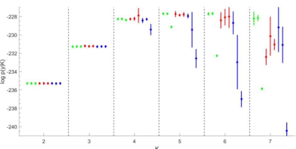
Figure 1 Marginal likelihood estimation for theGALAXYDATAoverK=2toK=7.For eachK,

5.1.1 Univariate Gaussian mixtures. For illustration, marginal likelihoods are computed for univariate Gaussian mixtures yi|Si = k ∼ N(μk, σk2) for the

GALAXY DATA (Richardson and Green, 1997) for K=2, . . . ,7, using the pri-ors μk ∼N(m, R2), σ_k2 ∼G−1(2, C0), and C0 ∼G(0.2,10/R2), where m and

R are the midpoint and the length of the observation interval. For a given

K, full conditional Gibbs sampling is performed by iteratively sampling from

Frühwirth-Schnatter(2006).

Results of marginal likelihood estimation are visualised in Figure1. There is a striking difference in the reliability of the nine estimators, in particular as K

increases. (Optimal) bridge sampling in combination with the fully symmetric importance density q_KF(ϑ) and the importance density q_KD(ϑ) (first two estima-tors in green) yield the most reliable results. Up to K=5, the dual IS estimator logpISˆ ,F(y|K) is as good as logpBSˆ ,F(y|K) and logpBSˆ ,D(y|K). However, for

K ≥6, the standard errors of both bridge sampling estimators are considerably smaller than the standard errors of the dual IS estimator due to their robustness with respect to the tail behaviour of the importance density. Reciprocal importance sampling estimators logpRIˆ ,•(y|K)(in blue) become particularly unreliable asK

increases, with extreme bias and huge SE, even for the fully symmetric importance densityq_KF(ϑ).

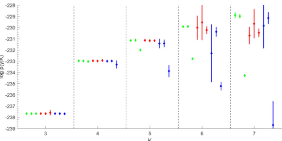
5.1.2 Multivariate Gaussian mixtures. For further illustration, marginal likeli-hoods are computed for multivariate Gaussian mixtures as in Section 4.1for the well-known FISHER’SIRISDATAforK=2, . . . ,5. We use the normal priorμk∼

(20)

N(my,Sy) and the hierarchical inverse Wishart prior k∼W−1(c0,C0), C0∼

W(g0, g0/φSy−1)where my is the componentwise median andSy is the sample

covariance matrix of the data,c0=2.5+(d−1)/2 andg0=0.5+(d−1)/2, with

d=4 being the dimension of the data, andφ=(1−R2)(c0−(d+1)/2), where

R2=0.5 is the amount of explained heterogeneity (Frühwirth-Schnatter, 2006). Results of marginal likelihood estimation are visualised in Figure 2. Again, (optimal) bridge sampling in combination with the fully symmetric importance density q_KF(ϑ) and the importance density q_KD(ϑ) yields the very reliable esti-mators logpBSˆ ,F(y|K)and logpBSˆ ,D(y|K). Up to K=4, the dual IS estimator

logpISˆ ,F(y|K) is as good as these estimators. However, forK=5, the standard

errors of the bridge sampling estimators are considerably smaller than the stan-dard errors of the dual IS estimator due to their robustness with respect to the tail behaviour of the importance density. Also for this example, the simple random bridge sampling estimator logpBSˆ ,R(y|K)and all reciprocal importance sampling

estimators logpRIˆ ,•(y|K)are substantially biased forK≥4.

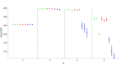
5.1.3 Poisson mixtures. Finally, marginal likelihoods are computed for Pois-son mixtures as in Section 4.1 for the EYE TRACKING DATA (Escobar and West, 1998) forK=3, . . . ,7 under a Gamma prior witha0=y2/(s_y2−y2)and

b0 =a0/y (Frühwirth-Schnatter, 2006). Results of marginal likelihood

estima-tion are visualised in Figure 3. Once more, the (optimal) bridge sampling esti-mators logpBSˆ ,F(y|K) and logpBSˆ ,D(y|K) are very precise even for increasing

(21)

5.2 Hidden Markov and Markov switching models for time series analysis

For illustration, we apply the estimators introduced in Section 4.2 to two time series analyzed inFrühwirth-Schnatter(2006). The prior of the transition matrixξ

is defined withep=4 andet =1/(K−1)and the initial valueS0 is assumed to

follow a uniform distribution.

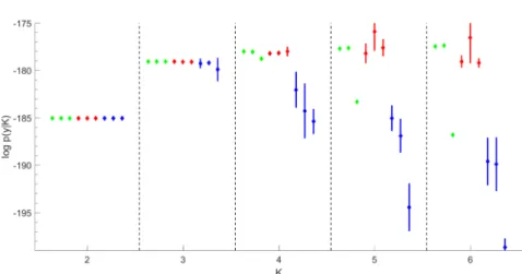
5.2.1 Hidden Markov models for the LAMBDATA. A Markov mixture of Pois-son distribution,yi|Si=k∼P(μk), is applied to the LAMBDATA, a time series of

count data (Leroux and Puterman, 1992), under the priorμk∼G(1,0.5). Marginal

likelihoods are computed forK=2, . . . ,6 and visualised in Figure4.

Using simple random permutation estimators, Frühwirth-Schnatter (2006), p. 353, reports quite unstable estimators of the marginal likelihood forK=4, lead-ing to chooseK=3 based on the BS and the RI estimator, whereas the IS estimator indicates K=4. Instability beyond K=3 is also evident in Figure 4, reporting nine different estimators for eachK. Also for Markov mixtures, the only reliable estimators of the marginal likelihood are logpˆBS,F(y|K)and logpˆBS,D(y|K)(the

first two estimators in green), based on (optimal) bridge sampling in combination with the fully symmetric importance density q_KF(ϑ) and the importance density

q_KD(ϑ). Up toK=4, the dual IS estimator logpISˆ ,F(y|K)(first estimator in red)

is as good as these estimators.

However, as for finite mixtures, forK≥5 the standard errors of this estimator are considerably larger than for the two BS estimators due to its lack of robustness with respect to the tail behaviour of the importance density. Once more, recipro-cal importance sampling estimators logpRIˆ ,•(y|K)become particularly unreliable

(22)

asK increases, with extreme bias and huge SE even for the fully symmetric im-portance densityq_KF(ϑ). The ever increasing marginal likelihood obtained through balanced bridge sampling indicates that the state-specific distribution might be misspecified and more flexible distributions, for example, a negative binomial dis-tribution should be considered.

5.2.2 Markov switching models for GDP analysis. A fully Markov switching model of order p with K states is fitted to the GDP DATA as in Frühwirth-Schnatter(2006), assuming that conditional onSi=k,

yi=δk,1yi−1+ · · · +δk,pyi−p+ζk+εi,

where εi|Si =k∼N(0, σ_ε,k2 ). Priors are chosen as δk,j ∼N(0,0.25), j =1,2,

ζk∼N(0,10), andσε,k2 ∼G−1(2,0.5).

For illustration, marginal likelihoods are computed forp=2 forK=1, . . . ,4 and visualised in Figure5. Also for this Markov switching model, the estimators logpˆBS,F(y|K) and logpˆBS,D(y|K)based on (optimal) bridge sampling in

com-bination with the fully symmetric importance densityq_KF(ϑ) and the importance densityq_KD(ϑ)are very precise, whereas all alternative estimators exhibit consider-ably larger standard errors and/or considerable bias. The presence ofK=2 states is clearly confirmed by this analysis.

5.3 Mixture of experts models in model-based clustering of time series

In many areas of applied statistics, like biometrics, economics, finance, psycho-metrics, public health, or in social sciences, data are available in the form of panel

(23)

Figure 5 Marginal likelihood estimation for theGDP DATAoverK=1toK=4.For eachK,

or longitudinal data where, for a given sample of subjects, repeated measurements are taken for a set of variables at several points in time. Standard methods for panel or longitudinal data analysis assume homogeneity across the subjects (Diggle et al., 2002). To capture (unobserved) heterogeneity across subjects, model-based clustering has been applied where each time series is considered to belong to one ofK unknown clusters, where each cluster is described by a different data gen-erating mechanism, see, for example,Frühwirth-Schnatter and Kaufmann(2008) andFrühwirth-Schnatter(2011).

To apply model-based clustering, one has to choose the clustering kernel

p(yi|θk)and the prior class assignment distribution Pr(Si=k|ω)fork=1, . . . , K.

To address serial dependence among the observations for each subject, model-based clustering of time series data is often model-based on dynamic clustering kernels derived from first-order homogeneous or inhomogeneous Markov processes, see Frühwirth-Schnatter(2011) for a review.

Assuming Pr(Si =k|ω)=ηk as for finite mixtures would imply that all

sub-jects have the same prior probability to belong to a certain cluster, regardless of their specific characteristics. To achieve more flexibility, covariatesxiare allowed

to influence the weight distribution, modeled as in (16) through a multinomial logit (MNL) model. Such mixture of experts models have been applied to model-based clustering of time series in combination with dynamic regression clustering ker-nels (Frühwirth-Schnatter and Kaufmann, 2008), Markov chain clustering kernels (Frühwirth-Schnatter et al., 2012), and locally independent MNL clustering ker-nels (Aßmann and Boysen-Hogrefe, 2011).