A weighted multiple classifier framework based on random projection.

(1)

NGUYEN, T.T., DANG, M.T., LIEW, A. W.-C. and BEZDEK, J.C. 2019. A weighted multiple classifier framework based on random projection. Information science [online], 490, pages 36-58. Available from:

https://doi.org/10.1016/j.ins.2019.03.067

A weighted multiple classifier framework based

on random projection.

NGUYEN, T.T., DANG, M.T., LIEW, A. W.-C. and BEZDEK, J.C.

2019

This document was downloaded from

https://openair.rgu.ac.uk

(2)

A weighted multiple classifier framework based on Random Projection

Tien Thanh Nguyen1_{, Manh Truong Dang}1_{, Alan Wee-Chung Liew}2_{, James C. Bezdek}3 1_{School of Computing Science and Digital Media, Robert Gordon University, Aberdeen, Scotland,}

United Kingdom

2_{School of Information and Communication Technology, Griffith University, Australia} 3_{Computer Science and Information Technology Department, University of Melbourne, Australia}

Abstract: In this paper, we propose a weighted multiple classifier framework based on random projections. Similar to the mechanism of other homogeneous ensemble methods, the base classifiers in our approach are obtained by a learning algorithm on different training sets generated by projecting the original up-space training set to lower dimensional down-spaces. We then apply a Least Square-based method to weigh the outputs of the base classifiers so that the contribution of each classifier to the final combined prediction is different. We choose Decision Tree as the learning algorithm in the proposed framework and conduct experiments on a number of real and synthetic datasets. The experimental results indicate that our framework is better than many of the benchmark algorithms, including three homogeneous ensemble methods (Bagging, RotBoost, and Random Subspace), several well-known algorithms (Decision Tree, Random Neural Network, Linear Discriminative Analysis, K Nearest Neighbor, L2-loss Linear Support Vector Machine, and Discriminative Restricted Boltzmann Machine), and random projection-based ensembles with fixed combining rules with regard to both classification error rates and F1 scores.

Keywords: Ensemble method, random projection, multiple classifier system, weighted multiple classifier.

(3)

Ensemble methods have been shown to achieve higher classification accuracy than single classifier systems and have been applied to many applications such as object detection and tracking, computer-aided medical diagnosis, and intrusion detection [48]. In general, ensemble methods can be categorized into two types [27]:

• Heterogeneous ensemble method: A set of diverse learning algorithms are used on one training set to generate different classifiers and decisions are made based on the output of these classifiers [28, 29]. This approach focuses on designing the algorithm that combines the outputs of the base classifiers to achieve higher accuracy than any single base classifier.

• Homogeneous ensemble method: A set of classifiers are generated by a single learning algorithm on different training sets obtained from an original one. The outputs of these classifiers are then combined to give the final decision. Several well-known homogeneous ensemble methods are Bagging [5], Boosting [15], Random Subspace [18], and Random Forest [6].

In this paper, we focus on the homogeneous ensemble method. In the literature, research on homogeneous ensemble methods can be divided into three aspects:

• Design of new ensemble systems: Several recent research efforts have focused on designing new ensemble systems [4, 31-33, 41]. Verma and Rahman generated an ensemble of classifiers based on clustering data at multi-layers [31] as well as the learning of clustering boundaries [41]. Rodriguez et al. [32] proposed the Rotation Forest in which principal component analysis (PCA) is applied to each of the subsets randomly selected from a feature set. The axis rotations form the new features for a base classifier. Schclar and Lokach [33] built ensemble system on training set schemes generated from a training set by using random matrices. Blaser and Fryzlewicz [4] designed a novel ensemble system by generating random rotation matrices to rotate the feature space before generating the base classifiers. Zhang et al. [45] combined Rotation Forest and AdaBoost in a single method named RotBoost which inherits the advantage of both ensembles for the classification tasks.

(4)

• Enhancing ensemble methods: This approach focuses on techniques to enhance the performance of Bagging, Boosting, Random Subspace, and Random Forest. For example, several classifier selection or redundant classifier pruning methods were proposed such as dynamic classifiers selection [7], instance-based pruning [17], ordered aggregation-based pruning [26], and semi-definite programming [46]. There are also hybrid approaches to weigh base classifiers in Random Subspace [44], and weigh feature subspaces in Bagging [9]. Several methods have been introduced to improve the performance of AdaBoost, for example by maximizing the margin between training samples of different classes via linear programming in LPBoost [12], and learning from skewed training data in RUSBoost [34] to handle imbalanced datasets. Besides the well-known combining algorithms like Sum and Majority Vote [29], novel combiners were introduced to enhance the task of combining on classifiers’ outputs. For example, Kuncheva et al. [21] used Ordered Weighted Averaging (OWA) operators to aggregate the classifiers’ outputs. Wang et al. [42] proposed a new fusion scheme based on upper integrals.

• Study on properties of the ensemble: The research look at properties of an ensemble such as diversity, margin, and generalization error bound, and their relationships. For instance, Kuncheva et al. [22] studied ten diversity measures among binary classifiers and examined the relationships between the accuracy and measures of diversity. Tang et al. [38] theoretically analyzed six diversity measures to understand the relations between them and the concept of margin. Gao and Zhou [16] obtained a tight generalization error bound by considering the empirical average margin and margin variance. Shi et al. [36] studied the preservation of margin after projecting data by random matrices. Wang et al. [43] studied the relationship between the model’s generalization ability and fuzziness of fuzzy classifiers. Kuncheva et al. [20] derived bounds with a kappa-error diagram which is used to analyze the performance of ensemble systems. Cannings et al. [10] introduced some theoretical results under some assumptions for the ensemble method generated by learning base classifiers on the projected data. Unlike our approach, the outputs of these classifiers are combined via the threshold-based voting method. The results include the difference in the expected

(5)

classification error rate between the random projection ensemble classifier and its infinite-simulation counterpart, and the bound for the difference between the expected error rate and the Bayes risk. The authors also derived results for specific choices of base classifier such as

Linear Discriminative Analysis, K Nearest Neighbor, and Quadratic Discriminative Analysis.

In this paper, we develop a homogeneous ensemble framework in which the training set schemes are generated by projecting the original training set to lower dimension spaces. A learning algorithm then learns the base classifiers on the down-space schemes. Further, we propose a technique to weigh the outputs of the base classifiers when combining them to generate the final prediction. We assume that each classifier is associated with a suitable weight, and our experiments will show that the proposed method performs better than un-weighted combining methods. Although random projection has been used to generate homogeneous ensemble systems before, to our knowledge, this is the first work that uses a weighted combination for random projection-based ensemble systems. Here we weigh the base classifiers by exploiting the relationship between the output of base classifiers on the training observations (called meta-data or Level 1 data) and their class labels via the Least Square method. It is noted that the technique to obtain the meta-data and the combiner is actually based on a heterogeneous ensemble technique known as stacking. As a result, the proposed method can be viewed as a combination of two approaches: homogeneous ensemble system (multiple base classifiers from one learning algorithm) and heterogeneous ensemble system (a learnable combiner obtained via stacking).

The paper is organized as follows. In section 2, we briefly discuss random projection and methods to weigh base classifiers in ensemble systems. In section 3, we develop our weighted multi-classifiers system based on random projections and regression. Experimental studies are presented in section 4 in which we conduct experiments on twenty-three datasets and compare the results of the proposed framework to a number of benchmark algorithms. Our conclusions and suggestions for further research appear in the last section.

(6)

2. Preliminary

2.1. Random Projection

In 1984, Johnson and Lindenstrauss (JL) published a paper about extending Lipschitz continuous maps from metric spaces to Euclidean spaces and introduced the JL Lemma [19]. The lemma begins with a linear transformation from a -dimensional space ℝ (called upspace) to a -dimensional space ℝ (called down-space). Specifically, given a finite set of -dimension data = , , … , ⊂ ℝ , they considered a linear transformation T: ℝ → ℝ : = T = , , … , ⊂ ℝ and = T . The linear transformation T can be represented in the form of matrix = T = so that if each element of the matrix is generated according to a specified random distribution, T is known as a random projection [30].

Random projections have three important properties:

• Random projections are useful in dimension reduction since the dimension of the down-space can always be chosen to be lower than that of up-space, i.e. < . In some situations, random projection is more preferred than Principle Component Analysis (PCA). First, random projection is independent of the data while PCA are data-dependent. This is useful in situations where data cannot be accessed all at once, such as in data streaming or online learning. Moreover, generating the principle components is computationally expensive compare to generating the random matrix in random projection [3].

• Fern and Brodley [14] indicated that random projections are very unstable since the dataset schemes generated from a data source based on random matrices are quite different. This property is important since other sampling methods like bootstrapping only generate slightly different dataset schemes. Thus an ensemble system based on a set of random projections offers a potential for increased diversity.

(7)

• Random projection can preserve in probability the pairwise distance between pairs of points in the up-space and down-space with a specified distortion level [11]. Specifically, the JL Lemma asserts that the distance between two data points in the down-space is bounded above and below by (1 ± ), respectively, with probability 1 − 1 #⁄ if the dimension of the down-space is greater than or equal to a target dimension _% (also called the JL bound). Here the value of _% only depends on the number of observations # and , and does not depend on the dimension ( ) of the up-space. Empirical evidence in [40] suggested that the bound given by ≥ _% = 2 × ln # ⁄ is the smallest value that ensures the distance preservation with probability 1 − 1 #⁄ .

These projections with bounded distortions are simply obtained by using a random matrix = 1 +⁄ ,-./0 of size × , where -_./ are random variables such that E2-./3 = 0 and Var2-./3 = 1. Several forms of are summarized in [2]:

• Plus-minus-one or Bernoulli random projection: = 1 +⁄ ,-./0 where -_./ is randomly chosen from −1, 1 such that Pr2-./= 13 = Pr2-./= −13 = 1 2⁄

• Achlioptas random projection: = 1 +⁄ ,-./0 where -_./ is randomly chosen in ,−√3, 0, √30 such that Pr2-_./ = √33 = Pr2-_./ = −√33 = 1 6⁄ and Pr2-./= √33 = 2 3⁄

• Normal random projection: = 1 +⁄ ,-./0 where -_./ is distributed according to a Gaussian distribution < 0, 1 .

2.2. Weighted combining methods

Fixed combining methods are frequently applied to the outputs of base classifiers to predict class labels. Popular fixed combing methods use fixed combining rules such as the Sum Rule, Product Rule, Min Rule, Max Rule, Median Rule and Majority Vote Rule [29]. An issue with fixed combining

(8)

rules is that the learners are treated equally in the aggregation step, i.e. all classifiers make an equal contribution in the final class label prediction.

In weighted combining methods, each classifier can put different weight on different class and the combining algorithm works by taking = weighted linear combinations of posterior probabilities for the = classes. The predicted class label for a new observation is then decided by selecting the maximum value among these combinations. Several methods have been proposed to find the weights. For example, Ting et al. [39] proposed MLR method which depends on solving = Linear Regression models corresponding to the = classes based on meta-data and the training data labels in crisp form to find these combining weights. Zhang and Zhou [47] proposed using linear programming to find the weights. Sen et al. [35] introduced a method that was inspired by MLR which uses a hinge loss function in the combiner instead of the conventional least square loss. Using this new function with regularization, three different combining methods were proposed, namely weighted sum, dependent weighted sum, and linear stacked generalization, based on different regularizations with group sparsity. Mao et al. [25] proposed three ways to weight classifiers in the ensemble by maximizing three different quadratic forms as the approximate objective functions of ensemble error with two constraints. Cai et al. [9] learned Bagging on different feature subspaces in which the weights were determined by minimizing classification error rate of Bagging with consideration on the combination of classification margins.

3. The proposed framework

We propose an ensemble framework for class label prediction using a weighted

multi-classifiers framework based on random projection (denoted as WMCRP). The ensemble of classifiers

is constructed by applying a learning algorithm on different training set schemes generated by projecting the original training set to several down-spaces. As random projection often generates significantly different training sets from an original training set [14, 30], system diversity is expected. To improve the classification performance, the weights of the base classifiers on each class label are learned by regressing between meta-data of training observations and their class labels. During

(9)

classification, an unlabeled observation is first projected onto each of the down-spaces. The feature vectors of the observation in the down-spaces are then classified by the base classifiers to generate the meta-data. The predicted class label is finally obtained by weighted linear combinations of the predictions of the base classifiers. The details are as follows.

During training, random matrices of size ( × ) denoted by _/ (> = 1, … , ) are generated. training set schemes _/ of size (? × ) are generated from the original training set of

size(? × )through the projection AB@ _/given by:

/= 2 /3 +C (1)

A learning algorithm D is then applied to each of the schemes _/ to obtain the base classifiersEF_/

> = 1, … , (see Figure 1).

A Cross Validation based procedure is used to learn the weight of each base classifiers for each class [28]. First, the training set G is divided into H disjoint parts G , … , GI , where G = G ∪ … ∪ GI, G.∩ G/= ∅ M ≠ > , and |G | ≈ ⋯ ≈ |GI|, and their corresponding GR , … , GRI in which GRS= G − GS. For each GR., we get training set data _/~. from _/ associated with GR.. The learning algorithm D then learns on _/~. to obtain classifier EF_/~. associated with GR_.. Projected observations in G_. denoted by _/. are then classified by EF_/~. to obtain the posterior probability reflecting how supportive a classifier is to a class label for the observation. Assuming that the number of training observations is ?, the output of the above procedure is an ? × = matrix U

U = V P W | ⋯ P WX| P W | ⋯ P WX| ⋮ ⋱ ⋮ ⋯ ⋯ ⋱ P[ W | ⋯ P[ WX| P[ W | ⋯ P[ WX| ⋮ ⋱ ⋮ P W | \ ⋯ P WX| \ ⋯ P[ W | \ ⋯ P[ WX| \ ] (2)

in which P_/ W_^| _. is the probability that _. belongs to class W_^ given by the >S_ classifier for each > = 1, … , ; ` = 1, … , = ; and ∑X_^b P_/ F^| = 1 [28, 29]. Since the class labels of the training observations are known in advance, the weights of the base classifiers on the class labels can be

(10)

learned by discovering the relationship between the meta-data and the class labels of the training observations. We denote the weight matrix c = ,d/^0 in which d/^ is the weight of the >S_ classifier on the `S_ class (> = 1, … , ; ` = 1, … , =) (see Table 1). The class memberships of an observation are obtained by a linear combination of the posterior probabilities and the associated weights as:

CM^ = ∑[/b d/^g/ W^| = ℙ^i^ (3)

in which ℙ^= jg W^| , g W^| , … , g_/ W_^| , … , g_[ W^| k and i^ = d ^, … , d[^ l

TABLE 1. THE MODEL OF WEIGHTED BASE CLASSIFIERS

Class 1 Class 2 … Class m … Class n

Classifier 1 g W | d g W | d … g W_^| d _^ … g W_X| d_X Classifier 2 g W | d g W | d … g W_^| d _^ … g W_X| d _X … … … … … Classifier o g_/ W | d_/ g_/ W | d_/ … g_/ W_^| d_/^ … g_/ W_X| d_/X … … … … … Classifier p g_[ W | d_[ g_[ W | d_[ … g_[ W_^| d_[^ g_[ W_X| d_[X CM CM … CM^ … CMX

The weight matrix is obtained by minimizing the difference between the class memberships of _. and its true class label. From meta-data U, we extract the prediction associated with the `S_ class as:

U^ = V P W^| ⋯ P[ W^| P W^| ⋯ P[ W^| ⋮ ⋱ ⋮ P W^| \ ⋯ P[ W^| \ ] (4)

(11)

Since the class label of is known in advance, we defined crisp label vector associated with the `S_ class as q^ = r_^ # = 1, … , ? in which r_^ is given by:

r^ = s1 if ∈ W_{0 otherwise}^ (5)

The weight vector i^ corresponding to the `S_ class label is then found by solving the following regression equation:

U^i^ = q^ (6)

The computation runs through ` = 1, … , = to obtain the × = weight matrix c = i^ . The process to obtain c is illustrated in Figure 2.

In the classification process, an unlabeled observation } is first projected to the down-spaces with the random projections , /0

/}= } /⁄+ , > = 1, … , (7)

Next, the base classifier ,EF/0 works on _/} to obtain its meta-data. Specifically, the meta-data of }, i.e. U } , is given by:

U } _{= ~}P W |

} _{⋯ P WX|} }

⋮ ⋱ ⋮

P[ W | } ⋯ P[ WX| }

• (8)

The combining algorithm is then applied to U } by considering the weight matrix c (3). Finally, the predicted class label is obtained by getting the label corresponding to the maximum value of class memberships:

(12)

Fig. 1 Training architecture for generating the base classifiers

Fig. 2 Architecture for finding the weights for the base classifiers

Remark 1: Regression equation (6) can be solved by the least square approach, i.e. by minimizing the sum-of-square errors functionℒ^

ℒ^ = ‖U^i^− q^‖ → min (10) Training set G Learning Algorithm Scheme Scheme _[ †[ EF[ EF … … Learning Algorithm EF~ EF[~ EF~I EF[~I Meta-data U RegressionU i = q RegressionU i = q RegressionUXiX= qX … … … … U U UX Scheme Scheme _[ ~ [~ … ~I [ ~I … … [ I [ I _… c i ‡ ‡X

(13)

Different constraints can be imposed on im such as: Non-Negative Least Squares, i.e. d_/≥ 0 [24, 37], Bounded Variable Least Squares, i.e. ˆ/≥ d_/≥ ‰/ in which ˆ/ and ‰_/ are given upper and lower bounds of d_/ [8], and Bounded Variable with Constant Sum, i.e. −1 < d/< 1, ∑[_/b d/= 1 [47]. We have the following proposition when the proposed method is applied to binary classification problems.

Proposition 1: In binary classification problems, if iŠandi‹associated with class labels W and W solve equation (6) by minimizing (10) with the constraint ∑[_/b d_/= 1, then iŠ= i‹

Proof: In the case of binary classification, from meta-dataU, we separate Uinto two ? × matrices UŠ and U‹ associated with the two class labels. Based on the property of posterior probability ∑X^b P/ F^| = 1, we have UŠ+ U‹= •, where•is? × matrix of ones. From the definition of qŠandq‹we haveqŠ+ q‹= ŠandŠis the ? × 1 vector of ones. We solve (10) to find iŠas: ‖U i − q ‖ → min

⇔ ‖ • − U i − Š − q ‖ → min ⇔ ‖•i − Š − U i − q ‖ → min

Because isatisfies the constraint ∑[_/b d_/= 1, we have •i − Š = •, where •isa ? × 1 vector of zeros. Therefore ‖U i − q ‖ ⇔ ‖U i − q ‖ that is the two optimization problems have same solutions □

Based on the result of Proposition 1, if the weight vector i is assumed to satisfy the constraint ∑[/b d/ = 1, we only need to solve (10) once to find the weight vectors associated with both class labels.

Remark 2: As mentioned earlier, the pairwise distance between the observations in the up-space and down-space is nearly preserved (in probability) with distortion level 1 ± if the dimension of the down-space is greater than or equal to a target dimension _%. The bound _% only depends on the

(14)

number of observations and and does not depend on the dimension of the up-space. However, this means that if a dataset has a large number of observations but with low feature dimension, _% can be greater than . In this paper, the dimension of the down-space is set to be = ⌈ %⌉ if ⌈ %⌉ < , and = 2⁄ otherwise. Here the value of = ⌈ _%⌉ is the smallest integer greater than the JL bound _% = 2 × ln # ⁄ .

Our algorithm is summarized as follows:

Algorithm: WMCRP: a weighted multiple classifier framework based on

random projection. Training Process

Input: Training set: G, dimension of down-space: , number of projections: , learning algorithm: D

Output: Base classifiers: EF_/, weights: c, and random matrix:

/, (> = 1, … , )

Step 1 (Random matrices, training set schemes, and base classifiers generation)

For >=1 to

Generate random matrix _/

Training set scheme _/= 2 /3 +C Base classifier EF_/ = Learn(D, _/) End

Step 1 (Meta-data generation) U = ∅

G , … , GI =T-partition G For eachG_.

GR. = G − G. For >=1 to

Obtain _/~. and _/. from / according to the partition GR. and G.

ClassifierEF_/~. = Learn(D, _/~.) U = U ∪Classify2EF_/~., _/.3

(15)

End For

Step 2 (Weight vector generation)

For `=1 to =

Get U_^ by (4) Compute q^ by (5) Find i^= ,’/^0

/b ,…,[ = arg mini ‖U^i − q^‖ with

constraint c = c ∪ i^ End

Return ,EF/0, c, , /0, (> = 1, … , )

Testing process

Input _{Unlabeled observation} }_{, base classifier},EF/0_{, random} matrix , /0, and weight vector c = i^ , (> = 1, … , and

` = 1, … , =)

Output Predicted class label for }

Step1: _{(Computing posterior probabilities for} }₎ For o=1 to

_/} = } _/⁄+

U } = Classify(EF_/, _/}) End For

Step2: (Generate class memberships for })

For `=1 to = CM^ } = ∑[_/b d/^P_/ W^| } End } _{∈ W} S if € = arg max_{^b ,…,X}CM_^ }

4. Experiments

4.1. Datasets

We evaluated WMCRP on twenty-three datasets from the UCI Machine Learning Repository (http://archive.ics.uci.edu/ml/datasets.html). Information about the datasets is summarized in Table 2.

(16)

TABLE 2. INFORMATION OF DATASETS IN EVALUATION Dataset # of features # of observations # of classes

Arcene 10000 200 2 Balance 4 625 3 Conn-Bench-Vowel 10 528 11 Hill-Valley 100 2424 2 Ionosphere 34 351 2 Iris 4 150 3 Letter 16 20000 26 Libras 90 360 15 Musk2 166 6598 2 Optdigits 64 5620 10 Page Blocks 10 5472 5 Penbased 16 10992 10 Phoneme 5 5404 2 Ring 20 7400 2 Tae 20 151 3 Tic-Tac-Toe 9 958 2 Thyroid 21 7200 3 Vehicle 18 946 4 Vertebral 6 310 3 Waveform_w_Noise 40 5000 3 Waveform_wo_Noise 21 5000 3 Wine-Red 11 1599 6 Wine-White 11 4898 7

4.2. Benchmark Algorithms and Experimental Settings

We performed an extensive comparison study with several well-known algorithms to validate our approach. Since our proposed framework belongs to the homogeneous ensemble-based approach in which several different training set schemes are generated from an original training set though random projections, we compared with three homogeneous ensemble methods namely Bagging [5], Random Subspace [18], and RotBoost [45]. We used C4.5 Decision Tree with prunned option as the learning algorithm in all the methods to construct the base classifiers [27]. As Decision Tree classifier returns only the class label of an observation, we used the method of [1] to obtain the class posterior probabilities needed for the combiner. In brief, it consists of first computing the algebraic distance of an observation to the class decision boundary induced by the learned Decision Tree, and then performing kernel-based density estimation on the computed algebraic distances to estimate the class posterior probabilities needed for the combiner.

In addition, to show the advantage of weighted combiner approach, we also compared WMCRP with six fixed combining ensemble systems based on random projection [29, 33] (denoted by RP Sum Rule, RP Product Rule, RP Max Rule, RP Min Rule, RP Median Rule, and RP Majority Vote Rule) .

(17)

To construct the ensemble for both WMCRP and the six fixed combining ensemble systems, we used plus-minus-one-based random projections in which the level of distort is set to 0.25 [30]. Finally, we compared WMCRP to six well-known learning algorithms, namely K-Nearest Neighbors (the

number of nearest neighbors is set to 5, denote by kNN5), Decision Tree, Linear Discriminative

Analysis (denoted by LDA), L2-loss Linear Support Vector Machine (denoted by L2LSVM, with

optimal value for the parameter “ provided by the package LIBLINEAR at: https://www.csie.ntu.edu.tw/~cjlin/liblinear/), Discriminative Restricted Boltzmann Machines (denoted by DRBM) [23], and Random Neural Network (denoted by RNN, with optimal values for the parameters provided by PRTools v.5 at: http://prtools.org/).

In this study, we constructed 10 and 200 base classifiers for WMCPR and all the benchmark algorithms except the six single-classifier learning algorithms (The subscript in the name of method denotes the number of base classifiers used in the ensemble). Ten base classifiers are the smallest number of base classifiers for a homogeneous ensemble system [32], while following [27] we selected the number of base classifiers as 200 for large ensembles. Non-Negative Least Squares [24, 37] is used to find the weight vector from equation (6). All source codes were implemented in Matlab running on a PC with Intel Core i5 with 2.5 GHz processor and 4G RAM. The sources are available at: https://github.com/ThanhNguyenRGU/RPWeight

4.3. Comparison criteria and methodology

We performed 10-fold CV and repeated it 10 times to obtain 100 test results for each dataset. Note that the 10-fold CV in the experiment is not related to the 10-fold CV procedure used to generate the meta-data. Besides using classification error rate as a performance measure, we also computed the F1 score. In this paper, we reported the mean and variance of classification error rate and F1 score computed on 100 tests on each dataset. Let #^/ be the number of observations from the `S_ class predicted to belong to the >S_ class. The classification error rate is given by:

Error Rate = 1 − ∑–•—˜ ••

(18)

The Precision, Recall and F1 score associated with the `S_ class are computed as: Precision^= •• ∑–@—˜ @• (12) Recall^= •• ∑– _•@ @—˜ (13) F1^ = ×›œ•žŸ Ÿ¡¢•×£•ž¤¥¥• ›œ•žŸ Ÿ¡¢•¦£•ž¤¥¥• (14)

The F1 score on a test set is the average value on all F1_^

F1 =_X∑X F1^

^b (15)

We used the Wilcoxon signed rank test [13] to assess the statistical significance of the difference between the classification results (error rate or F1 score) of WMCRP and the benchmark algorithms on each dataset. Here we test the null hypothesis, i.e. “two methods perform equally” on each experimental dataset. Denote §. as the difference between the performance scores of the proposed method and a benchmark algorithm on the MS_ output of ¨ test sets (in this study ¨ is equal 100). The differences are ranked according to their absolute values and averaged ranks are assigned in cases of no difference. Let ©¦ and ©ª be the sum of ranks for §_. > 0 and §_. < 0, respectively.

©¦_{= ∑}_- _{rank §.}

®¯% + ∑-®b%rank §. (16)

©ª_{= ∑}_- _{rank §.}

®°% + ∑-®b%rank §. (17)

Let © be the smaller of the sums

For large ¨, the distribution of the statistic

± = ²ª˜³´ ´¦

(19)

will be approximately normal. The performance scores of two methods are treated as significantly different if the g − ¹º»ˆ¼ of the test is smaller than a given confident level ½. In our experiments, ½ was set to 0.05.

4.4. Results and Discussions

4.4.1. Classification error rate comparison

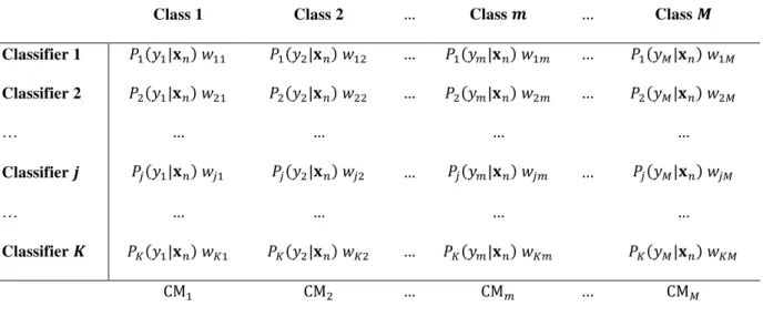
The classification error rates of the benchmark algorithms and WMCRP are shown in Tables A1-A5. The statistical test result displayed in Figure 3 shows that WMCRP is better than the benchmark algorithms (The detail of the statistical test results can be found in Tables S1-S2 in the supplement material). Comparing WMCRP200 to Bagging200, we rejected 19 null hypotheses that the

two methods perform equally. In 12 of the 19 cases, the classification error rates of WMCRP200 are

smaller than that of Bagging200. WMCRP200 also significantly outperforms Random Subspace200 (17

wins against 6 loses). The statistical test results clearly demonstrate the advantage of using random projections to construct the ensemble system. The WMCRP200 is also better than six random

projection-based ensemble systems using fixed combining rules i.e. RP Sum Rule200 (10 wins against

6 loses), RP Product Rule200 (22 wins against 1 lose), RP Max Rule200 (22 wins against 1 lose), RP

Min Rule200 (22 wins against 1 lose), RP Median Rule200 (14 wins against 5 loses), and RP Majority

Vote Rule200 (10 wins against 6 loses). This demonstrates the benefit of weighted combining methods

over fixed combining methods in ensemble systems.

When using only 10 base classifiers, the proposed method is competitive to Bagging and RP Sum and is better than the other homogeneous ensemble methods. Moreover, WMCRP10 still

outperforms six well-known learning algorithms i.e. ¾NN5 (13 wins against 8 loses), Decision Tree

(15 wins against 5 loses), DRBM (13 wins against 9 loses), RNN (15 wins against 4 loses), LDA (14 wins against 4 loses), and L2LSVM (14 wins against 6 loses). In overall, WMCRP10 has 17.39 wins

against 2.89 losses in average. In other words, it beats the other 15 methods in about 64.81% of the tests. Similarly, the advantage of using WMCRP200 against the other 15 benchmark algorithms is

(20)

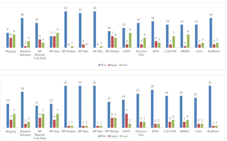
4.4.2. F1 Score comparison

For the F1 score, the statistical test results in Figure 4 exhibit a similar trend to those in Figure 3 (The F1 score can be found in the Appendix from Tables A6-A10. The detail of the statistical test results can be found in Tables S3-S4 in the supplement material). WMCRP200 is better than Bagging

and significantly better than Random Subspace. Compare to random projection-based ensembles using fixed combining rules, WMCRP200 also outperforms RP Sum Rule200 (12 wins against 7 loses)

and RP Majority Vote Rule200 (11 wins against 7 losses) while significantly outperforms RP Product

Rule200, RP Max Rule200, RP Min Rule200 (21 wins against 1 lose in all the cases), and RP Median

Rule200 (13 wins against 5 loses). The comparisons in the case of using 10 base classifiers also show

the superior performance of WMCRP to the benchmark algorithms. Overall, WMCRP10 has 15.1333

wins against 4.7333 losses on average. In other words, it beats the other 15 methods in about 66.57% of the tests. Similarly, the advantage of using WMCRP200 against the other 14 classifiers is about

72.43%.

The success of WMCRP can be explained by two reasons. First, the random projection creates a set of diverse data schemes from that of the up-space. This allows an ensemble of classifiers to be learned from the projected data. The smaller dimension of the projected data in the down-spaces also reduces the adverse effect of the curse of dimensionality. Therefore, ensemble systems built on random projection can obtain better classification performance. Moreover, we propose a method to weigh the base classifiers of the ensemble system, and a weighted combining mechanism further improves the classification performance of random projection-based ensemble.

It is interesting to see how WMCRP performs on datasets with a large number of features but a small number of instances. For this, we examine its performance on the Arcene dataset, which has 10000 features but only 200 instances. Our method (both WMCRP10 and WMCRP200) is better than

Decision Tree, RotBoost, RNN, and three RP fixed rule methods (Product, Max, Min) for both classification error rate and F1 Score. It is comparable to Bagging and ¾NN5, but underperforms

DRBM, Random Subspace, L2LSVM, and three RP fixed rule methods (Sum, Median, Majority). Therefore, for this kind of dataset, our method does not have a clear advantage over the benchmark algorithms we compared with, i.e. it outperforms six benchmark algorithms, underperforms six benchmark algorithms, and is comparable with the other two benchmark algorithms.

(21)

Fig. 3 Statistical test results comparing WMCRP10 (top figure) and WMCRP200 (bottom figure) to the benchmark algorithms for classification error rate 9 16 15 3 22 22 22 9 13 16 16 14 13 14 17 6 1 6 14 0 1 0 10 2 3 4 3 1 1 3 8 6 2 6 1 0 1 4 8 4 3 6 9 4 3 Bagging Random Subspace RP Majority Vote Rule RP Sum Rule RP Product Rule RP Max Rule RP Min Rule RP Median Rule kNN5 Decision Tree RNN L2LSVM DRBM LDA RotBoost

Win Equal Lose

12 17 10 10 22 22 22 14 15 18 19 17 15 16 20 4 0 7 7 0 0 0 4 6 2 2 2 4 1 2 7 6 6 6 1 1 1 5 2 3 2 4 4 2 1 Bagging Random Subspace RP Majority Vote Rule RP Sum Rule RP Product Rule RP Max Rule RP Min Rule RP Median Rule kNN5 Decision Tree RNN L2LSVM DRBM LDA RotBoost

(22)

Fig. 4 Statistical test results comparing WMCRP10 (top figure) and WMCRP200 (bottom figure) to the benchmark algorithms for F1 score 9 18 15 7 22 21 22 10 12 15 16 ₁₄ ₁₄ ₁₄ 18 6 1 5 7 0 2 0 7 2 2 4 2 1 2 2 8 4 3 9 1 ₀ 1 6 9 6 3 7 8 3 3 Bagging Random Subspace RP Majority Vote Rule

RP Sum RP Product RP Max RP Min RP Median kNN5 Decision Tree

RNN L2LSVM DRBM LDA RotBoost

Win Equal Lose

12 18 11 12 21 21 21 13 14 17 19 16 16 15 21 4 2 5 4 1 1 1 5 7 3 2 3 3 2 1 7 3 7 7 1 1 1 5 2 3 2 4 4 2 1 Bagging Random Subspace RP Majority Vote Rule

RP Sum RP Product RP Max RP Min RP Median kNN5 Decision Tree

RNN L2LSVM DRBM LDA RotBoost Win Equal Lose

(23)

4.4.3. Time complexity analysis

Let ¿ D denotes the complexity of the learning algorithm D which learns on training set schemes to obtain the base classifiers, the complexity of the learning process of the proposed method

is ¿ Àmax ÀH × D, Áprojection matrix _generation Ä , Ádown space _{projection Ä , Á}weight vector_{computation ÄÈÈ} in which ¿ H × D

is the time complexity of generating meta-data of training set via running H-fold Cross Validation, ¿ Áprojection matrix _generation Ä is the time complexity of random matrix generation, ¿ Ádown space _{projection Ä} is the time complexity to project training set to down spaces, and Áweight vector

computation Ä is the time complexity to find the weight vectors. In this study, we used plus-minus-one random projection so that only × comparisons are needed to generate a × random matrix _/. Hence the complexity of random matrix generation is ¿ × × . The training set of size (? × )is projected to down space to obtain a new training set scheme _/ of size (? × ) through matrix multiplication, i.e. _/ = 2 /3 +C . The computational complexity of matrix multiplication for and _/ is ¿ ? × × . Therefore, the time complexity of matrix multiplications is ¿ × ? × × . Finally, the time complexity of finding weight vectors through Least Squares is ¿ = × × ? . Therefore, the time complexity of the learning process of the proposed method is ¿ max H × D, × ? × ×

, = × × ? . The proposed method can also be implemented via parallel processors to reduce time complexity.

Table A11 in the Appendix shows the average training and classification time (in seconds) of the proposed method and the 3 homogeneous ensemble methods (Bagging, Random Subspace, and RotBoost) using 200 base classifiers computed on 100 training sets and the associated test sets partitioned from 8 selected datasets. Although the proposed method generally has much longer training time and also longer classification time than these benchmark algorithms due to the meta-data generation process, the differences are within practical limit.

(24)

4.4.4. The effect of using different learning algorithms

To see the effect of using different learning algorithm, we compare the performance of using LDA or kNN5 in place of Decision Tree in WMCRP. Fig 5 shows the mean classification error rates

and F1 Score of the 3 cases on the 23 UCI datasets (The detailed results can be found in Table S5 and S6 in the supplement material). Unlike other ensemble methods such as Bagging which requires unstable base classifiers or AdaBoost which requires weak classifiers to construct the ensemble, any learning algorithms can be used in WMCRP to generate the base classifiers. Due to the unstable properties of the random projection, the generated training sets on the down-space are very different. As a result, there is no constraint on the type of learning algorithms for the random projection-based ensemble.

Obviously, using different learning algorithms will result in different performance. Overall, WMCRP(kNN5) is the best method, obtaining the best classification error rate and F1 Score on 10

datasets. On some datasets such as Letter and Penbased, WMCRP(kNN5) is significantly better than

the others (0.0355, 0.0567, and 0.2475 for the classification error rate of WMCRP(kNN5),

WMCRP(Decision Tree), and WMCRP(LDA), respectively, on the Letter dataset). Decision Tree is also an effective learning algorithm when combining with random projection in WMCRP as WMCRP(Decision Tree) outperforms the others on 9 datasets for both classification error rate and F1 Score. Meanwhile, WMCRP(LDA) is the poorest among the 3 learning methods and obtains the best performance measures on only 4 datasets. As different learning algorithms obtain the best results on different datasets, a framework that first selects the best learning algorithms and then weighs the base classifiers is, therefore, a promising way to further improve the performance of the ensemble on diverse data sources.

(25)

Fig.5 Classification error rate and F1 Score of the proposed method with 3 different learning algorithms 0.0 0.1 0.2 0.3 0.4 0.5 0.6

Classification Error Rate

WMCRP (LDA) WMCRP(kNN(5)) WMCRP(Decision Tree)

0.0 0.1 0.2 0.3 0.4 0.5 0.6 0.7 0.8 0.9 1.0 F1 Score

(26)

5. Conclusions

We have introduced WMCRP, a weighted ensemble-based classification framework based on random projections and least square regression. Our approach generates training sets from the original data based on random projections, and then uses a learning algorithm, here a Decision Tree, to learn the base classifiers on the down-space projections. The weights for combining the outputs of the base classifiers are obtained by solving a non-negative linear least squares problem using the meta-data of the training observations and their crisp class labels. Experimental results on twenty-three UCI datasets demonstrated the benefit of our approach compared with 15 other well-known algorithms for both classification error rate and F1 score. Specifically, in our experiments the proposed method is better than the three homogeneous ensemble methods (i.e. Bagging, RotBoost, and Random Subspace), six ensemble systems based on random projections and fixed combining rules (i.e. RP Sum Rule, RP Product Rule, RP Max Rule, RP Min Rule, RP Median Rule, and RP Majority Vote Rule), and six well-known learning algorithms (i.e. ¾NN5, LDA, Decision Tree, DRBM, L2LSVM,

and RNN). We believe that WMCRP can be fruitfully combined with feature selection as well as the learning algorithm selection to further improve its classification performance. This will be our next immediate research focus.

References

[1] I. Alvarex, S. Bernard, G. Deffuant, Keep the Decision Tree and estimate the class probabilities using its decision boundary, in Proc. IJCAI, 2007, pp. 654-659.

[2] R. Avogadri, G. Valentini, Fuzzy ensemble clustering based on random projections for DNA microarray data analysis, Artificial Intelligence in Medicine.45 (2009), 173-183.

[3] E. Bingham, H. Mannila, Random projection in dimensionality reduction: applications to image and text data, in Proc. 7th Int. Conf. on Knowledge discovery and data mining (ACM SIGKDD), 2001, pp. 245-250.

(27)

[4] R. Blaser, P. Fryzlewicz, Random Rotation Ensemble, Journal of Machine Learning Research.2 (2015), 1-15.

[5] L. Breiman, Bagging Predictors, Machine Learning. 24 (1996), 123-140. [6] L. Breiman, Random Forest, Machine Learning. 45 (2001), 5-32.

[7] A.S. Britto Jr., R. Sabourin, L.E.S. Oliveira, Dynamic selection of classifiers-A comprehensive review, Pattern Recognition. 47(11) (2014), pp. 3665–3680.

[8] R. Brol, S. De Jong, A fast non-negativity-constrained least squares algorithm, Journal of Chemometrics. 11(5) (1997), 393–401.

[9] Q.T. Cai, C.Y. Peng, C.S. Zhang, A weighted subspace approach for improving bagging performance, in Proc. of IEEE ICASSP, USA, 2008, pp. 3341–3344.

[10] T.I. Cannings, R.J. Samworth, Random-projection ensemble classification, Journal of the Royal Statistical Society: Series B: Statistical Methodology. 79(4) (2017), 959-1035.

[11] S. Dasgupta, A. Gupta, An elementary proof of the Johnson Lindenstrauss lemma, in Proc. ACM SIGMOD-SIGACT-SIGART, 2002, pp.274–281.

[12] A. Demiriz, K.P. Bennett, J.S. Taylor, Linear Programming Boosting via Column Generation, Machine Learning. 46 (2002), pp. 225-254.

[13] J. Demsar, Statistical comparisons of classifiers over multiple datasets, Journal of Machine Learning Research. 7 (2006), 1–30.

[14] X.Z. Fern, C.E. Brodley, Random Projection for High Dimensional Data Clustering: A Cluster Ensemble Approach, in Proc. 20th Int. Conf. on Machine Learning (ICML), 2003, pp 186-193.

[15] Y. Freund, R.E. Schapire, Experiments with a new boosting algorithm, in: Proceedings of International Conference on Machine Learning (ICML), 1996, pp. 148-156.

[16] W. Gao, Z.H. Zhou, On the doubt about margin explanation of boosting, Artificial Intelligence. 203 (2013), pp. 1–18.

(28)

[17] D. Hernandez-Lobato, G. Martinez-Muoz, A. Suarez, Statistical instance-based pruning in ensembles of independent classifiers, IEEE Transactions on Pattern Analysis and Machine Intelligence. 31(2) (2009), 364-369.

[18] T.K. Ho, The random subspace method for constructing decision forests, IEEE Transactions on Pattern Analysis and Machine Intelligence. 20(8) (1998), 832-844.

[19] W. Johnson, J. Lindenstrauss, Extensions of Lipschitz mapping into Hilbert space, Conference in modern analysis and probability, vol. 26 of Contemporary Mathematics, American Mathematical Society, 1984, pp. 189-206.

[20] L.I. Kuncheva, A Bound on Kappa-Error Diagrams for Analysis of Classifier Ensembles, IEEE Transactions on Knowledge and Data Engineering. 25(3) (2013), pp. 494-501.

[21] L.I. Kuncheva, Combining Pattern Classifiers: Methods and Algorithms Second Edition, Wiley Press, 2014.

[22] L.I. Kuncheva, C.J. Whitaker, Measures of Diversity in Classifier Ensembles and Their Relationship with the Ensemble Accuracy, Machine Learning. 51 (2003), 181–207.

[23] H. Larochelle, Y. Bengio, Classification using Discriminative Restricted Boltzmann Machines, in Proc. 25th Int. Conf. on Machine Learning (ICML), 2008, pp. 536-543.

[24] C.L. Lawson, R.I. Hanson, Solving Least Squares Problems, SIAM Publisher, 1995

[25] S. Mao, L. Jiao, L. Xiong, S. Gou, B. Chen, S.-K. Yeung, Weighted classifier ensemble based on quadratic form, Pattern Recognition. 48(5) (2015), 1688–1706.

[26] G. Martinez-Muoz, D. Hernandez-Lobato, A. Suarez, An analysis of ensemble pruning techniques based on ordered aggregation, IEEE Transactions on Pattern Analysis and Machine Intelligence. 31(2) (2009), 245-259.

[27] T.T. Nguyen, T.T.T. Nguyen, X.C. Pham, A.W.C. Liew, A Novel Combining Classifier Method based on Variational Inference, Pattern Recognition. 49 (2016), 198-212.

[28] T.T. Nguyen, M.P. Nguyen, X.C. Pham, A.W.C. Liew, A Hybrid Classification System with Fuzzy Rule and Classifier Ensemble, Information Sciences. 422 (2018), 144-160.

(29)

[29] T.T. Nguyen, X.C. Pham, A.W.C. Liew, W. Pedrycz, Aggregation of Classifiers: A Justifiable Information Granularity Approach, IEEE Transactions on Cybernetic. (2018), DOI 10.1109/TCYB.2018.2821679.

[30] M. Popescu, J. Keller, J. Bezdek, A. Zare, Random Projections Fuzzy C-Mean (RPFCM) for big data clustering, in Proc. IEEE Int. Conf. on Fuzzy System, 2015.

[31] A. Rahman, B. Verma, Novel layered clustering-based approach for generating ensemble of classifiers, IEEE Transactions on Neural Network. 12(5) (2011), 781-792.

[32] J.J. Rodriguez, L.I. Kuncheva, C.J. Alonso, Rotation Forest: A New Classifier Ensemble Method, IEEE Transactions on Pattern Analysis and Machine Intelligence. 28(10) (2006), 1619-1630. [33] A. Schclar, L. Rokach, Random Projection Ensemble Classifiers, in: J. Filipe, J. Cordeiro, Enterprise Information Systems, Lecture Notes in Business Information Processing, Springer Berlin Heidelberg, 2009, pp 309-316.

[34] C. Seiffert, T. Khoshgoftaar, J. Hulse, A. Napolitano, RUSBoost: Improving classification performance when training data is skewed, in Proc. 19rd Int. Conf. on Pattern Recognition, 2008, pp. 1–4.

[35] M.U. Şen, H. Erdogˇan, Linear classifier combination and selection using group sparse regularization and hinge loss, Pattern Recognition Letters. 34(3) (2013), 265–274

[36] Q. Shi, C. Shen, R. Hill, A.V.D. Hengel, Is margin preserved after random projection?, in Proc. 29th Int. Conf. on Machine Learning (ICML), 2012, pp 591-598.

[37] P.B. Stark, R.L. Parker, Bounded-variable least-squares: an algorithm and applications, Computational Statistics. 10 (1995), 129–129.

[38] E.K. Tang, P.N. Suganthan, X. Yao, An analysis of diversity measures, Machine Learning. 65(1) (2006), 247-271.

[39] K.M. Ting, I.H. Witten, Issues in stacked generalization, Journal of Artificial Intelligence Research. 10 (1999), 271-289.

[40] S. Ventkatasubramanian, Q. Wang, The Johnson-Lindenstrauss transform: An empirical study, in Proc. ALENEX, SIAM, 2011, pp. 164-173.

(30)

[41] B. Verma, A. Rahman, Cluster-oriented ensemble classifier: Impact of multicluster characterization on ensemble classifier learning, IEEE Transactions on Knowledge and Data Engineering. 24(4) (2012), 605-618.

[42] X.Z. Wang, R. Wang, H.M. Feng, H.C. Wang, A New Approach to Classifier Fusion Based on Upper Integral, IEEE Transactions On Cybernetics. 44(5) (2014), 620-635.

[43] X.Z. Wang, H.J. Xing, Y. Li, Q. Hua, C.R. Dong, W. Pedrycz, A study on relationship between generation abilities and fuzziness of base classifiers in ensemble learning, IEEE Transactions on Fuzzy Systems. 23 (5) (2015), 1638-1654.

[44] Z. Yu, L. Li, J. Liu, G. Han, Hybrid Adaptive Classifier Ensemble, IEEE Transactions on Cybernetics. 45(2) (2015), 177 - 190.

[45] C.X. Zhang, J.S. Zhang, RotBoost: A technique for combining Rotation Forest and AdaBoost, Pattern Recognition Letters. 29(10) (2008), 1524-1536.

[46] Y. Zhang, S. Burer, W. Nick Street, Ensemble pruning via semi-definite programming, Journal of Machine Learning Research. 7 (2006), 1315-1338.

[47] L. Zhang, W.D. Zhou, Sparse ensembles using weighted combination methods based on linear programming, Pattern Recognition. 44(1) (2011), 97-106.

(31)

Appendix

TABLE.A1. MEAN AND VARIANCE OF CLASSIFICATION ERROR RATES OF SIX LEARNING ALGORITHMS

ÉNN5 Decision Tree DRBM LDA L2LSVM RNN

Mean Variance Mean Variance Mean Variance Mean Variance Mean Variance Mean Variance

Arcene 0.1725 6.32E-03 0.2625 8.37E-03 0.1040 4.03E-03 - - 0.0980 4.75E-03 0.3525 9.32E-03

Balance 0.1502 1.32E-03 0.2101 1.61E-03 0.0701 7.71E-04 0.1297 6.08E-04 0.1273 6.24E-04 0.1011 4.99E-04

Conn-Bench-Vowel 0.0701 1.36E-03 0.2333 3.74E-03 0.3043 4.78E-03 0.3856 3.80E-03 0.5431 4.15E-03 0.1154 1.91E-03

Hill-Valley 0.3904 8.52E-04 0.3891 8.27E-04 0.2599 3.99E-03 0.3160 6.49E-04 0.0160 6.45E-05 0.3119 1.50E-03

Ionosphere 0.1593 2.51E-03 0.1242 2.57E-03 0.1169 3.24E-03 - - 0.1613 2.35E-03 0.1240 2.55E-03

Iris 0.0393 1.79E-03 0.0500 2.43E-03 0.0380 1.89E-03 0.0193 1.00E-03 0.0473 2.25E-03 0.0453 2.66E-03

Letter 0.0450 2.04E-05 0.1346 4.38E-05 0.4945 7.41E-04 0.2978 9.30E-05 0.2947 9.86E-05 0.2705 1.55E-04

Libras 0.2419 3.68E-03 0.3322 5.32E-03 0.4058 5.06E-03 0.3550 5.73E-03 0.4025 4.44E-03 0.2844 5.20E-03

Musk2 0.0345 4.70E-05 0.0320 4.86E-05 0.0056 1.69E-05 0.0566 6.39E-05 0.0508 5.96E-05 0.0793 7.36E-05

Optdigits 0.0124 2.10E-05 0.1023 2.01E-04 0.0693 8.73E-04 - - 0.0334 5.09E-05 0.0780 1.30E-04

Page-Blocks 0.0432 4.72E-05 0.0344 4.38E-05 0.1003 6.35E-06 0.0532 5.23E-05 0.0437 3.66E-05 0.0352 3.76E-05

Penbased 0.0074 5.44E-06 0.0418 4.16E-05 0.0669 2.34E-04 0.1252 8.46E-05 0.0822 7.28E-05 0.0365 4.95E-05

Phoneme 0.1140 1.74E-04 0.1331 1.69E-04 0.1620 2.14E-04 0.2409 2.35E-04 0.2455 2.28E-04 0.1530 1.90E-04

Ring 0.3083 1.68E-04 0.1162 1.53E-04 0.0223 2.75E-05 0.2374 2.33E-04 0.2606 1.52E-04 0.0926 2.25E-04

Tae 0.5929 1.40E-02 0.4347 1.07E-02 0.5137 1.60E-02 0.4790 1.41E-02 0.5830 9.90E-03 0.4847 1.32E-02

Tic-Tac-Toe 0.1570 6.89E-04 0.1388 1.55E-03 0.0372 2.64E-04 0.3088 1.26E-03 0.3122 9.80E-04 0.2449 1.95E-03

Thyroid 0.0600 1.78E-05 0.0042 5.61E-06 0.0457 2.85E-05 - - 0.0523 1.47E-05 0.0553 1.95E-05

Vehicle 0.3516 1.98E-03 0.2888 1.83E-03 0.3549 1.66E-03 0.2164 1.42E-03 0.2236 1.32E-03 0.2207 1.14E-03

Vertebral 0.1745 2.48E-03 0.2068 3.08E-03 0.1558 2.37E-03 0.1965 3.69E-03 0.1984 2.42E-03 0.1742 3.04E-03

Waveform-w-Noise 0.1879 2.57E-04 0.2535 3.63E-04 0.1470 2.67E-04 0.1397 2.27E-04 0.1346 1.89E-04 0.1846 3.72E-04

Waveform-wo-Noise 0.1804 2.63E-04 0.2487 3.12E-04 0.1369 2.24E-04 0.1397 1.91E-04 0.1399 2.41E-04 0.1718 2.49E-04

Wine-Red 0.4908 9.90E-04 0.4001 1.48E-03 0.4371 1.04E-03 0.4082 9.79E-04 0.4171 8.77E-04 0.4035 1.09E-03

Wine-White 0.5136 3.64E-04 0.4186 5.02E-04 0.5247 2.52E-04 0.4656 4.08E-04 0.5296 3.76E-04 0.4554 4.58E-04

(32)

TABLE.A2. MEAN AND VARIANCE OF CLASSIFICATION ERROR RATES OF SIX RANDOM PROJECTION-BASED FIXED COMBINING

RULES (USING 10 BASE CLASSIFIERS)

RP Sum Rule10 RP Product Rule10 RP Max Rule10 RP Min Rule10 RP Median Rule10 RP Majority Vote

Rule10 Mean Variance Mean Variance Mean Variance Mean Variance Mean Variance Mean Variance

Arcene 0.1880 8.41E-03 0.4380 5.91E-03 0.4380 5.91E-03 0.4380 5.91E-03 0.1865 8.94E-03 0.1845 8.78E-03

Balance 0.1312 2.21E-03 0.1141 1.88E-03 0.1033 1.90E-03 0.1101 1.56E-03 0.1963 6.25E-03 0.2313 8.34E-03

Ionosphere 0.0610 1.34E-03 0.2325 3.23E-03 0.2328 3.22E-03 0.2328 3.22E-03 0.0604 1.38E-03 0.0641 1.83E-03

Iris 0.0500 3.23E-03 0.1980 9.20E-03 0.1367 5.81E-03 0.1987 8.62E-03 0.0560 3.80E-03 0.0573 3.91E-03

Letter 0.1204 7.31E-05 0.7021 1.49E-04 0.3602 1.55E-04 0.7021 1.49E-04 0.1437 8.97E-05 0.1404 9.28E-05

Libras 0.1747 2.95E-03 0.6306 4.65E-03 0.3858 5.25E-03 0.6306 4.65E-03 0.1833 3.36E-03 0.1819 3.49E-03

Musk2 0.0398 4.83E-05 0.0788 4.72E-05 0.0788 4.72E-05 0.0788 4.72E-05 0.0398 4.88E-05 0.0432 4.80E-05

Optdigits 0.0319 4.51E-05 0.4966 4.48E-04 0.2531 3.29E-04 0.4966 4.48E-04 0.0390 6.90E-05 0.0356 5.78E-05

Penbased 0.0152 1.71E-05 0.2620 3.01E-04 0.1426 1.22E-04 0.2620 3.01E-04 0.0157 1.52E-05 0.0158 1.67E-05

Phoneme 0.1380 2.65E-04 0.2893 5.95E-04 0.2894 5.92E-04 0.2894 5.92E-04 0.1378 2.85E-04 0.1385 2.73E-04

Ring 0.0420 4.83E-05 0.2396 2.12E-04 0.2396 2.12E-04 0.2396 2.12E-04 0.0426 4.53E-05 0.0454 4.49E-05

Tae 0.4267 1.24E-02 0.3903 1.11E-02 0.4340 1.57E-02 0.3956 1.19E-02 0.4380 1.35E-02 0.4478 1.38E-02

Thyroid 0.0561 2.27E-05 0.1984 2.12E-04 0.1696 1.99E-04 0.1984 2.13E-04 0.0563 2.73E-05 0.0565 2.58E-05

Vehicle 0.3301 1.93E-03 0.6189 1.09E-03 0.4078 1.53E-03 0.6189 1.08E-03 0.3287 2.20E-03 0.3305 1.96E-03

Wine-Red 0.3715 1.14E-03 0.6285 1.11E-03 0.4049 9.43E-04 0.6290 1.10E-03 0.3727 1.14E-03 0.3783 1.01E-03

(33)

TABLE.A3. MEAN AND VARIANCE OF CLASSIFICATION ERROR RATES OF TWO HOMOGENEOUS ENSEMBLE METHODS AND PROPOSED

METHOD (USING 10 BASE CLASSIFIERS)

WMCRP10 Bagging10 Random Subspace10

Mean Variance Mean Variance Mean Variance

Arcene 0.2130 9.93E-03 0.2090 8.02E-03 0.1765 5.77E-03 Balance 0.0880 1.36E-03 0.1682 1.11E-03 0.2504 3.00E-03 Conn-Bench-Vowel 0.1006 2.00E-03 0.1468 2.31E-03 0.1864 3.52E-03 Hill-Valley 0.1281 7.64E-04 0.3568 8.10E-04 0.3643 9.73E-04 Ionosphere 0.0672 1.67E-03 0.0920 2.50E-03 0.0860 1.85E-03 Iris 0.0467 2.18E-03 0.0527 2.60E-03 0.0593 3.37E-03 Letter 0.1252 6.54E-05 0.0807 5.30E-05 0.2375 1.03E-03 Libras 0.2008 3.70E-03 0.2606 4.55E-03 0.2511 4.37E-03 Musk2 0.0396 4.75E-05 0.0258 3.84E-05 0.0290 3.43E-05 Optdigits 0.0329 5.58E-05 0.0503 1.04E-04 0.1273 5.66E-04 Page-Blocks 0.0411 4.00E-05 0.0294 3.16E-05 0.0364 8.26E-05 Penbased 0.0150 1.63E-05 0.0222 2.26E-05 0.0532 9.61E-05 Phoneme 0.1349 2.49E-04 0.1070 1.56E-04 0.1797 4.18E-04 Ring 0.0426 4.91E-05 0.0645 8.08E-05 0.1000 1.17E-04 Tae 0.4431 1.74E-02 0.4325 1.34E-02 0.5171 1.44E-02 Thyroid 0.0559 2.05E-05 0.0039 5.44E-06 0.0602 5.45E-05 Tic-Tac-Toe 0.0916 3.11E-03 0.0822 6.91E-04 0.3087 7.56E-04 Vehicle 0.3270 2.07E-03 0.2596 1.61E-03 0.2871 1.93E-03 Vertebral 0.1903 3.78E-03 0.1887 2.67E-03 0.2910 6.08E-03 Waveform-w-Noise 0.1858 3.24E-04 0.1871 2.86E-04 0.2954 1.10E-03 Waveform-wo-Noise 0.1702 2.92E-04 0.1851 2.32E-04 0.2293 6.03E-04 Wine-Red 0.3734 1.19E-03 0.3386 1.14E-03 0.3580 9.03E-04 Wine-White 0.3789 4.05E-04 0.3530 4.86E-04 0.3735 4.50E-04

(34)

TABLE.A4. MEAN AND VARIANCE OF CLASSIFICATION ERROR RATES OF SIX RANDOM PROJECTION-BASED FIXED COMBINING

RULES (USING 200 BASE CLASSIFIERS)

RP Sum Rule200 RP Product Rule200 RP Max Rule200 RP Min Rule200 RP Median Rule200 RP Majority

Vote Rule200 Mean Variance Mean Variance Mean Variance Mean Variance Mean Variance Mean Variance

Arcene 0.1285 4.96E-03 0.5600 4.00E-04 0.5600 4.00E-04 0.5600 4.00E-04 0.1265 4.97E-03 0.1275 5.02E-03

Balance 0.1067 4.70E-04 0.1438 1.32E-03 0.0811 1.36E-03 0.1441 1.31E-03 0.1256 9.43E-04 0.1430 1.08E-03

Iris 0.0407 2.30E-03 0.4980 7.42E-03 0.3140 5.27E-03 0.4980 7.42E-03 0.0427 2.54E-03 0.0407 2.57E-03

Letter 0.0530 2.50E-05 0.8564 3.17E-05 0.7492 5.40E-05 0.8564 3.17E-05 0.1253 5.38E-05 0.0553 2.95E-05

Libras 0.1369 2.63E-03 0.7742 3.07E-03 0.6597 4.28E-03 0.7742 3.07E-03 0.1558 2.81E-03 0.1328 2.79E-03

Musk2 0.0369 4.86E-05 0.1238 3.61E-05 0.1238 3.61E-05 0.1238 3.61E-05 0.0367 4.69E-05 0.0368 4.70E-05

Penbased 0.0085 6.73E-06 0.7086 1.36E-04 0.5578 1.76E-04 0.7086 1.36E-04 0.0094 7.61E-06 0.0083 7.25E-06

Phoneme 0.1155 1.73E-04 0.6319 1.06E-04 0.6319 1.06E-04 0.6319 1.06E-04 0.1152 1.59E-04 0.1150 1.64E-04

Ring1 0.0205 2.20E-05 0.4936 2.67E-06 0.4936 2.67E-06 0.4936 2.67E-06 0.0209 2.39E-05 0.0206 2.25E-05

Tae 0.4074 1.38E-02 0.3678 1.04E-02 0.3703 1.15E-02 0.3750 9.64E-03 0.4054 1.51E-02 0.4153 1.64E-02

Thyroid 0.0548 1.98E-05 0.6785 3.18E-04 0.6405 3.30E-04 0.6785 3.18E-04 0.0543 2.12E-05 0.0541 2.14E-05

Vehicle 0.3146 1.82E-03 0.7365 3.03E-04 0.5655 1.14E-03 0.7365 3.03E-04 0.3143 1.89E-03 0.3109 1.81E-03

Wine-Red 0.3558 1.02E-03 0.7134 1.07E-03 0.5754 1.21E-03 0.7134 1.07E-03 0.3567 1.01E-03 0.3608 9.75E-04

(35)

TABLE.A5. MEAN AND VARIANCE OF CLASSIFICATION ERROR RATES OF THREE HOMOGENEOUS ENSEMBLE METHODS AND

PROPOSED METHOD (USING 200 BASE CLASSIFIERS)

WMCRP200 Bagging200 Random Subspace200 RotBoost

Mean Variance Mean Variance Mean Variance Meam Variance

Arcene 0.1705 6.70E-03 0.1730 6.97E-03 0.1390 6.98E-03 0.2530 7.89E-03 Balance 0.0713 8.76E-04 0.1605 8.38E-04 0.2134 1.71E-03 0.1440 9.76E-04 Conn-Bench-Vowel 0.0312 6.09E-04 0.1016 1.94E-03 0.0699 1.26E-03 0.3230 5.25E-03 Hill-Valley 0.0290 1.28E-04 0.3230 9.49E-04 0.3311 8.68E-04 0.3608 1.37E-03 Ionosphere 0.0570 1.49E-03 0.0932 2.27E-03 0.0775 2.00E-03 0.1157 2.76E-03 Iris 0.0393 1.96E-03 0.0440 2.42E-03 0.0540 3.17E-03 0.0453 2.21E-03 Letter 0.0567 3.52E-05 0.0599 3.09E-05 0.1016 6.13E-05 0.1413 7.06E-05 Libras 0.1367 2.28E-03 0.2136 4.13E-03 0.1933 3.02E-03 0.4367 6.59E-03 Musk2 0.0342 4.67E-05 0.0214 2.77E-05 0.0220 2.41E-05 0.1289 1.49E-04 Optdigits 0.0161 2.84E-05 0.0389 7.08E-05 0.0389 8.52E-05 0.0637 1.50E-04 Page-Blocks 0.0378 4.33E-05 0.0272 3.20E-05 0.0313 3.19E-05 0.0634 7.60E-05 Penbased 0.0074 5.82E-06 0.0179 1.71E-05 0.0225 2.12E-05 0.0592 9.97E-05 Phoneme 0.1144 1.29E-04 0.0945 1.30E-04 0.1600 2.30E-04 0.1860 3.93E-04 Ring 0.0232 2.63E-05 0.0551 7.34E-05 0.0315 2.89E-05 0.1122 2.66E-04 Tae 0.4139 1.61E-02 0.3923 1.66E-02 0.5218 1.16E-02 0.5366 1.41E-02 Tic-Tac-Toe 0.0211 1.85E-04 0.0592 5.67E-04 0.3067 4.23E-04 0.2846 9.48E-04 Thyroid 0.0529 2.48E-05 0.0038 5.84E-06 0.0632 8.93E-06 0.0280 8.02E-05 Vehicle 0.2901 1.70E-03 0.2575 1.74E-03 0.2625 1.53E-03 0.3332 2.70E-03 Vertebral 0.1806 4.06E-03 0.1781 2.36E-03 0.2619 4.08E-03 0.1858 3.10E-03 Waveform-w-Noise 0.1398 2.32E-04 0.1619 2.56E-04 0.1715 2.48E-04 0.1678 2.60E-04 Waveform-wo-Noise 0.1374 1.91E-04 0.1597 2.32E-04 0.1525 2.11E-04 0.1606 2.71E-04 Wine-Red 0.3509 9.15E-04 0.3061 8.67E-04 0.3176 8.30E-04 0.4120 1.26E-03 Wine-White 0.3534 3.82E-04 0.3095 5.20E-04 0.3279 3.28E-04 0.4418 2.93E-04

(36)

TABLE.A6. MEAN AND VARIANCE OF F1 SCORE OF SIX LEARNING ALGORITHMS

ÉNN5 Decision Tree DRBM LDA L2LSVM RNN

Mean Variance Mean Variance Mean Variance Mean Variance Mean Variance Mean Variance

Arcene 0.8232 6.61E-03 0.7307 8.68E-03 0.8938 4.22E-03 - - 0.8997 4.98E-03 0.6365 9.59E-03

Balance 0.6052 6.67E-04 0.5631 8.21E-04 0.8257 5.73E-03 0.6043 2.85E-04 0.6035 2.98E-04 0.6623 4.11E-03

Ionosphere 0.8046 4.90E-03 0.8648 3.09E-03 0.8662 4.46E-03 - - 0.8059 4.77E-03 0.8570 3.79E-03

Iris 0.9602 1.83E-03 0.9491 2.58E-03 0.9615 1.94E-03 0.9805 1.02E-03 0.9494 2.33E-03 0.9542 2.70E-03

Letter 0.9548 2.06E-05 0.8653 4.36E-05 0.4548 1.36E-03 0.7018 9.28E-05 0.6739 1.10E-04 0.7275 1.59E-04

Libras 0.7412 4.94E-03 0.6461 5.52E-03 0.5441 6.84E-03 0.6195 6.77E-03 0.6708 5.75E-03 0.6964 6.13E-03

Musk2 0.9309 2.10E-04 0.9382 1.84E-04 0.9892 6.33E-05 0.8825 3.14E-04 0.9061 2.40E-04 0.8133 5.65E-04

Optdigits 0.9876 2.10E-05 0.8978 2.01E-04 0.9277 1.48E-03 - - 0.9674 4.68E-05 0.9220 1.32E-04

Penbased 0.9926 5.40E-06 0.9583 4.14E-05 0.9322 2.95E-04 0.8728 8.81E-05 0.9149 7.04E-05 0.9637 4.89E-05

Phoneme 0.8601 2.60E-04 0.8395 2.49E-04 0.8040 2.89E-04 0.6952 4.11E-04 0.7083 3.47E-04 0.8144 2.63E-04

Ring 0.6568 3.05E-04 0.8838 1.53E-04 0.9777 2.75E-05 0.7609 2.43E-04 0.7232 2.25E-04 0.9072 2.27E-04

Tae 0.3943 1.51E-02 0.5499 1.21E-02 0.4698 1.75E-02 0.5034 1.57E-02 0.4311 1.26E-02 0.5002 1.48E-02

Thyroid 0.6075 1.68E-03 0.9761 2.05E-04 0.7321 1.99E-03 - - 0.5672 9.38E-04 0.6394 1.93E-03

Vehicle 0.6395 2.05E-03 0.7096 1.83E-03 0.6120 2.19E-03 0.7799 1.55E-03 0.7651 1.63E-03 0.7777 1.23E-03

Wine-Red 0.2408 6.53E-04 0.3169 1.56E-03 0.2101 2.30E-04 0.3170 4.26E-03 0.2168 3.48E-04 0.2735 5.13E-04

Wine-White 0.2483 6.48E-04 0.3336 5.89E-04 0.1495 9.13E-05 0.2809 2.00E-03 0.1380 4.42E-05 0.2138 1.47E-04

(37)

TABLE.A7. MEAN AND VARIANCE OF F1 SCORE OF SIX RANDOM PROJECTION-BASED FIXED COMBINING RULES (USING 10 BASE

CLASSIFIERS)

RP Sum Rule10 RP Product Rule10 RP Max Rule10 RP Min Rule10 RP Median Rule10 RP Majority

Vote Rule10 Mean Variance Mean Variance Mean Variance Mean Variance Mean Variance Mean Variance

Arcene 0.8071 8.90E-03 0.5058 1.21E-02 0.5058 1.21E-02 0.5058 1.21E-02 0.8086 9.47E-03 0.8121 9.16E-03

Balance 0.6373 6.93E-03 0.7616 1.06E-02 0.7558 1.49E-02 0.7645 1.01E-02 0.5822 8.07E-03 0.5723 1.33E-02

Iris 0.9494 3.32E-03 0.7949 1.09E-02 0.8566 7.13E-03 0.7940 1.02E-02 0.9432 3.94E-03 0.9416 4.11E-03

Letter 0.8792 7.37E-05 0.3983 2.22E-04 0.6378 1.59E-04 0.3983 2.22E-04 0.8679 6.92E-05 0.8607 8.76E-05

Libras 0.8143 3.63E-03 0.3894 7.16E-03 0.5772 6.44E-03 0.3894 7.16E-03 0.8083 3.91E-03 0.8052 4.34E-03

Musk2 0.9153 2.71E-04 0.8058 4.93E-04 0.8058 4.93E-04 0.8058 4.93E-04 0.9152 2.72E-04 0.9065 2.87E-04

Penbased 0.9849 1.71E-05 0.7857 2.02E-04 0.8571 1.30E-04 0.7857 2.02E-04 0.9844 1.50E-05 0.9842 1.67E-05

Phoneme 0.8270 4.70E-04 0.7008 5.45E-04 0.7007 5.42E-04 0.7007 5.42E-04 0.8276 5.02E-04 0.8330 3.96E-04

Ring 0.9580 4.83E-05 0.7450 3.00E-04 0.7450 3.00E-04 0.7450 3.00E-04 0.9573 4.53E-05 0.9546 4.50E-05

Tae 0.5637 1.31E-02 0.5960 1.29E-02 0.5544 1.70E-02 0.5902 1.41E-02 0.5518 1.49E-02 0.5402 1.56E-02

Thyroid 0.6423 2.05E-03 0.3909 4.47E-04 0.5671 6.67E-04 0.3908 4.50E-04 0.6459 2.17E-03 0.6609 1.86E-03

Vehicle 0.6649 1.91E-03 0.3285 2.19E-03 0.5577 1.86E-03 0.3286 2.15E-03 0.6697 2.11E-03 0.6633 1.95E-03

Wine-Red 0.3139 1.73E-03 0.2727 2.24E-03 0.3194 2.34E-03 0.2724 2.25E-03 0.3144 1.90E-03 0.3026 1.06E-03