Topology classification with deep learning to improve real-time event selection at the LHC

(1)

Topology classification with deep learning to improve

real-time event selection at the LHC

Thong Q. Nguyen

1

, Daniel Weitekamp III

2

, Dustin Anderson

1

, Roberto

Castello

3

_{, Olmo Cerri}

1

_{, Maurizio Pierini}

3

_{, Maria Spiropulu}

1

_{, and Jean-Roch}

Vlimant

1

_{California Institute of Technology (USA)}

2

_{University of California at Berkeley (USA)}

3

_{Experimental Physics Department, CERN (CH)}

Abstract

We show how event topology classification based on deep learning could be used to improve the purity of data samples selected in real time at at the Large Hadron Collider. We consider different data representations, on which different kinds of multi-class classifiers are trained. Both raw data and high-level features are utilized. In the considered examples, a filter based on the classifier’s score can be trained to retain∼99%of the interesting events and reduce the false-positive rate by as much as one order of magnitude for certain background processes. By operating such a filter as part of the online event selection infrastructure of the LHC experiments, one could benefit from a more flexible and inclusive selection strategy while reducing the amount of downstream resources wasted in processing false positives. The saved resources could be translated into a reduction of the detector operation cost or into an effective increase of storage and processing capabilities, which could be reinvested to extend the physics reach of the LHC experiments.

1 Introduction

The CERN Large Hadron Collider (LHC) collides protons every 25 ns. Each collision can result in any of hundreds of physics processes. The total data volume exceeds by far what the experiments could record. This is why the incoming data flow is typically filtered through a set of rule-based algorithms, designed to retain only events with particular signatures (e.g., the presence of a high-energy particle of some kind). Such a system, commonly referred to astrigger, consists of hundreds of algorithms, each designed to accept events with a specific topology. The ATLAS [1] and CMS [2] trigger systems are based on this idea. In their current implementation, given the throughput capability and the typical event size, these two experiments can write on disk∼1000events/sec. A few processes, e.g., QCD multijet production, constitute the vast majority of the produced events. One is typically interested to select a fraction of these events for further studies. On the other hand, the main interest of the LHC experiments is related to selecting and studying the many rare processes which occur at the LHC. In a typical data flow, these events are overwhelmed by the large amount of QCD multijet events. The trigger system is put in place to make sure that the majority of these rare events are part of the stored

∼1000events/sec.

Trigger algorithms are typically designed to maximize the efficiency (i.e., the true-positive rate), resulting in a non-negligible false-positive rate and, consequently, in a substantial waste of resources at trigger level (i.e., data throughput that could have been used for other purposes) and downstream (i.e., storage disk, processing power, etc.).

(2)

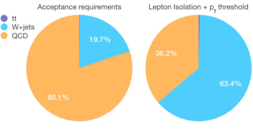
Figure 1: Relative composition of the isolated-lepton sample after the acceptance requirement (left) and the trigger selection (right), as described in the text.

The most commonly used selection rules areinclusive, i.e., more than one topology is selected by the same requirement. The so-called isolated lepton triggers are a typical example of this kind of algorithms. These triggers select events with a high-momentum electron or muon and no surrounding energetic particle, a typical signature of an interesting rare process, e.g., the production of aW boson decaying to a neutrino and an electron or muon. With such a requirement, one can simultaneously collectW bosons produced in the primary interaction (W events) or from the cascade decay of other particles, e.g., top quarks (mainly int¯tevents where a top quark-antiquark pair is produced). A sample selected this way is dominated byW events but it retains a substantial (>10%) contamination from QCD multijet. Thet¯tcontribution is smaller than1%. Events fromt¯tproduction are sometimes triggered by a set of dedicated lepton+jets algorithms, capable of using looser requirements on the lepton at the cost of introducing requirements on jets.1 _{Due to this additional complexity, the use of} these triggers in a data analysis comes with additional complications. For instance, the applied jet requirements produce distortions on offline distributions of jet-related quantities. To avoid having this effect, any typical data analysis applies a tighter offline selection. This means that many of the selected events close to the online-selection threshold are discarded. This is not necessarily the most cost-effective way to retain an unbiased dataset for offline analysis.

In this paper, we investigate the possibility of using machine learning to disentangle events from different event topologies at trigger level. Doing so, one could customize the trigger-selection strategy on individual processes (depending on the physics goals) while keeping the selection loose and simple. As a benchmark case, we consider a stream of data selected by requiring the presence of

one electron or muon with transverse momentumpT >23GeV2and a loose requirement on the

isolation. Details on the applied selection can be found in Sec. 2.

The considered benchmark sample is dominated by directWproduction, with a sizable contamination from QCD multijet events and a small contribution oft¯tevents. Other interesting processes (e.g.,

W W,W Z, andZZ production) are usually selected with more exclusive and dedicated trigger

algorithms (e.g., di-muon or di-electron triggers), or share the same kinematic properties of the two main interesting processes (Wandtt¯). For the sake of simplicity, we ignore these sub-leading processes in our study, without compromising the validity of our conclusions. Fig. 1 shows the composition of a sample with one electron or muon within the defined acceptance (pT >22GeV and

1

A jet is a spray of hadrons, typically originating from the hadronization of gluons and quarks produced in the proton collisions.

2

(3)

pseudorapidity|η|=| −log[tan(θ/2)]|<2.6, whereθis the polar angle), before and after applying the trigger requirements (pT >23GeV and loose isolation).

Such a loose set of requirements would translate into an event acceptance rate of∼690Hz for a luminosity of2×1034_cm−2_s−1_{, well beyond the currently allocated budget for these triggers. We}

suggest that, using the score of our topology classifier, one could tune the amount of each process to be stored for further analysis, within the boundaries of the allocated resources (typically∼200Hz). For instance, one might be interested to retain all thet¯tevents and some fraction ofWevents, while rejecting the QCD multijet events. We envision two main applications: for a given total rate, one could loosen the baseline trigger requirements, increasing the acceptance efficiency at no cost. Or, for a given acceptance efficiency (true positive rate), one could save resources by reducing the overll rate, rejecting the contribution of unwanted topologies (see Appendix A).

We consider several topology classifiers based on deep learning model architectures: fully-connected deep neural networks (DNNs), convolutional neural networks (CNNs) [3], and recurrent neural net-works such as Long-Short-Term-Memory netnet-works (LSTMs) [4] and gated recurrent units (GRUs) [5]. We consider four different representations of the collision events: (i) a set of physics-motivated high-level features, (ii) the raw image of the detector hits, (iii) a sequence of particles, characterized by a limited set of basic features (energy, direction, etc.), and (iv) anabstractrepresentation of this list of particles as an image.

The paper is structured as follows. In Sec. 2 we describe the four data representations. In Sec. 3 we describe the corresponding classification models. Results are discussed in Sec. 4. In Sec. 5 we inves-tigate the generalization properties of the four classifiers to scenarios of other topologies. In Sec. 6 we briefly discuss applications of machine learning algorithms to similar problems. Conclusions are given in Sec. 7. Appendix A describes a different scenario, in which the classifier is used to save resources by reducing the trigger acceptance rate, as opposed of using it to sustain a loose trigger selection that could otherwise require too many resources.

2 Dataset

Synthetic data corresponding toW,t¯tand QCD multijet production topologies are generated using

thePYTHIA8event generation library [6]. The setup of the proton-beam simulation is loosely inspired

by the LHC running configuration in 2015-2016: two proton beams, each with 6.5 TeV, generate on average 20 proton-proton collisions per crossing.

Generated samples are processed with theDELPHESlibrary [7], which applies a parametric model

of a detector response. Detector performances is tuned to the CMS upgrade design foreseen for the High-Luminosity LHC [8], as implemented in the corresponding default card provided withDELPHES. We run theDELPHESparticle-flow(PF) algorithm, which combines the information from all the CMS detector components to derive a list of reconstructed particles, the so-called PF candidates. For each particle, the algorithm returns the measured energy and flight direction. Each particle is associated to one of three classes: charged particles, photons, and neutral hadrons.

The basic event representation consists of a list of reconstructed PF candidates. For each candidate q, the following information is given: (i) The particle four-momentum in Cartesian coordinates (E, px,py,pz); (ii) The particle three-momentum in cylindrical coordinates: the transverse momentum

pT, the pseudorapidityη, and the azimuthal angleφ; (iii) The Cartesian coordinates (xvtx,yvtx,zvtx)

of the particle point of origin. For all neutral particles, (0, 0, 0) is used in the absence of pointing information; (iv) The electric charge; (v) The particle isolation with respect to charged particles

(ChPFIso), photons (GammaPFIso), or neutral hadrons (NeuPFIso). For each particle class, the

isolation is quantified as ISO= P p6=qp p T pq_T , (1)

where the sum extends over all the particles of the appropriate class with angular distance∆R= p

(∆η)2_{+ (∆}_φ₎2_<₀_.₃_{from the particle}_q_.

The particle identity is categorized via a one-hot-encoded representation (isChP ar,isN euHad, isGamma), corresponding to a charged particle, a neutral hadron, or a photon. In addition, two boolean flags are stored (isEleandisM u) to identify if a given particle is an electron or a muon. In total, each particle is then described by 19 features.

(4)

The trigger selection is emulated by requiring all the events to include one isolated electron or

muon with transverse momentumpT >23GeV and particle-based isolationChISO+GammaISO+

NeuISO <0.45. This baseline selection, which follows the typical requirements of an inclusive single-lepton trigger algorithm, accepts≈100QCD multijet events and≈176Wevents for everyt¯t event. Despite its largeW andt¯tefficiency, this trigger selection comes with a large cost in terms of QCD multijet events written on disk and processed offline. The cost is even larger if the main physics target ist¯tevents and theW contribution is seen as an additional source of background (e.g., in a high-statistics scenario, with all measurements ofW properties limited in precision by systematic uncertainties).

All particles are ranked in decreasing order ofpT. For each event, the isolated lepton is the first

entry of the list of particles. To avoid double counting of this isolated lepton`as a charged particle, each charged particleqis required to have∆R(q, `)>10−4. In addition to the isolated lepton, we consider the first 450 charged particles, the first 150 photons, and the first 200 neutral hadrons. This corresponds to a total of 801 particles per event, each characterized by the 19 features described above. If fewer particles are found in the event, zero padding is used to guarantee a fixed length of the particle list across different events. The events are then stored as numpy arrays in a set of compressed HDF5 files. The dataset is planned to be released on the CERN OpenData portal, accessible at

opendata.cern.ch.

In addition to this raw-event representation, we provide a list of physics-motivated high-level features, computed from the full event (theHLFdataset):

• ST, i.e. the scalar sum of thepT of all the jets, leptons, and photons in the event with

pT >30GeV and|η|<2.6. Jets are clustered from the reconstructed PF candidates, using

theFASTJET[9] implementation of the anti-kT jet algorithm [10], with jet-size parameter

R=0.4.

• The missing transverse energyEmiss

T , defined as the absolute value of the missing transverse

momentum, computed summing over the full list of reconstructed PF candidates: E_Tmiss=~p_Tmiss = −X q ~ p_Tq . (2)

• The squared transverse mass,M2

T, of the isolated lepton`and theETmisssystem, defined as:

MT2 = 2p`TEmissT (1−cos ∆φ) (3)

withp`

T the transverse momentum of the lepton and∆φthe azimuthal separation between

the lepton and~pmiss

T vector.

• The azimuthal angle of the~pmiss

T vector,φmiss.

• The number of jets entering theST sum.

• The number of these jets identified as originating from abquark.

• The isolated-lepton momentum, expressed in polar coordinates (pT,η,φ)

• The three isolation quantities (ChPFIso,NeuPFIso,GammaPFIso) for the isolated lepton.

• The lepton charge.

• TheisEleflag for the isolated lepton.

The list of 801 particles is used to generate two visual representations of the events. In the first one, the (η,φ) plane corresponding to the detector acceptance is divided into a barrel region (|η|<1.5), two end-cap regions (1.5≤η <3.0and−3.0< η≤ −1.5), and two forward regions (3.0≤η <5.0 and−5.0< η≤ −3.0). The barrel and endcap regions of the electromagnetic calorimeter, as well as the endcap of the hadronic calorimeter (HCAL), are binned in cells of size0.0187×0.0187. The barrel region of the HCAL is binned with cells of size0.087×0.087. The forward regions are binned with cells of size 0.175 inη, while the dimension inφvaries from 0.175 to 0.35. Each cell is filled with the scalar sum of thepT of the particles pointing to that cell. The three classes of particles

(charged particles, photons, and neutral hadrons) are considered separately, resulting in three adjacent images. An example is shown in Fig. 2 for at¯tevent. This representation corresponds to the raw image recorded by the detector.

(5)

Photons

Barrel Endcap Endcap

Forward Forward Forward Endcap Barrel Endcap Forward ForwardEndcap Barrel EndcapForward

Charged Tracks Neutral Hadrons

Figure 2: An example of at¯tevent as the input of the raw-image classifier.

Recently, it was proposed to represent LHC collision events as abstract images where reconstructed physics objects (jets, in that case) are represented as geometric shapes whose size reflects the energy of the particle [11]. We generalize this approach by applying it to the full list of particles. Each particle is represented as a unique geometric shape, centered at the particle’s(η, φ)coordinates and with size proportional to itslogpT. The geometric shapes are chosen as follow: (i) pentagons for the

selected isolated electron or muon; (ii) triangles for photons; (iii) squares for charged particles; (iv) hexagons for neutral hadrons. The images are digitized as arrays of size5×150×94, where each of the first four channels contains a separated particle class, and the last channel contains theEmiss

T ,

represented as a circle. As an example, the abstract representation for the event in Fig. 2 is shown in Fig. 3.

This abstract representation allows mitigating the sparsity problem of the raw images. On the other hand, there is no guarantee that the physics information is fully retained in this translation. As a result, there could be a reduction of discrimination power. This is one of the points we aim to investigate in this study.

(a) Photons (b) Charged Particles (c) Neutral Hadrons

(d) Lepton (e)Emiss

T

Figure 3: Example of at¯tevent, represented as a 5-channel abstract image.

3 Model description

In this section, we describe five types of multi-class classifiers, trained on the four data representations described in the previous section. We start by considering a state-of-the art HEP application, based on the high-level features listed in Sec. 2. We then consider a convolutional neural network taking as input the raw images. This model offers the baseline point of comparison for the classifier using the abstract images. In order to have a fair comparison between the two approaches, the same kind of network architecture is used for the two sets of images. Next, we consider recurrent neural networks based on LSTMs and GRUs, trained directly on the lists of 801 particles. Finally, we consider a

(6)

classifier taking both the high-level features and the list of 801 particles as inputs, using a combination of recurrent neural networks and fully connected neural networks.

The CNNs are implemented inPyTorch[12]. The recurrent neural networks and feed-forward

neural networks are implemented inKerasand trained usingTheano[13] as a back-end. The Adam

optimizer [14] is used to adapt the learning rate. The training is capped at 50 epochs, and can be stopped early if there is no improvement in terms of validation loss after 8 epochs. Categorical cross entropy is used as the loss function. All trainings are performed on a cluster of GeForce GTX 1080 GPUs. In an early stage of this work, experiments on the recurrent models were performed on the CSCS Piz Daint super computer, using thempi-learnlibrary [15] for multiple-GPU training.

3.1 High-level-features classifier using feed-forward neural networks

A fully connected feed-forward DNN based on a set of high-level features (HLF classifier) is the closest approach to the currently used rule-based trigger algorithms. We train a model of this kind taking as input the 14 features contained in the HLF dataset (see Sec. 2). The 14 features are normalized to take values between 0 and 1.

The final network configuration is the result of an optimization process performed using the

scikit-learn[16] optimizer, which performs an exhaustive cross-validated grid-search over a set

of hyperparameters related to the network architecture and the training setup. The number of layers, the number of nodes in each layer, and the choice of optimizer have been considered in the scan. For a given number of layers, discrimination performances were found to be constant over the considered range of number of nodes per layer. We believe that this is a direct consequence of the simple problem at hand: even a relatively small networks achieve good classification performances. We then took the smallest network as the best compromise between performance and architecture minimality. The chosen architecture consists of three hidden layers with 50, 20, and 10 nodes, activated by rectified linear units (ReLU) [17]. The output layer consists of 3 nodes, activated by a softmax activation function.

3.2 Raw-image and abstract-image classifiers using convolutional neural networks

To classify events represented as raw calorimeter images (raw-image classifier) and abstract images (abstract-image classifier), we use DenseNet-121, an instantiation of the Densely Connected Con-volutional Network [18]. The DenseNet-121 architecture includes 4 dense blocks, each of which contains 6, 12, 24, 16 dense layers, respectively. Each dense layer contains two 2D convolutional layers preceded by batch normalization layers. A dropout rate of 0.5 is applied after each dense layer. Between two subsequent dense blocks is a transition layer consisting of a batch normalization layer, a 2D convolutional layer, and an average pooling layer.

3.3 Particle-sequence classifier using recurrent neural networks

Aparticle-sequence classifieris trained using a recursive layer, taking as input the 801 candidates. To feed these particles into a recurrent network, particles are ordered according to their increasing or decreasing distance from the isolated lepton. Different physics-inspired metrics are considered to quantify the distance (∆R,∆φ,∆η,kT [10], or anti-kT [19]). The best results are obtained using

the∆Rdecreasing distance ordering.

We use gated recurrent units (GRU) to aggregate the input sequence of particle flow candidate features into a fixed size encoding. The fixed encoding is fed into a fully connected layer with 3 softmax activated nodes. Input data is standardized so that each feature has zero mean and unit standard deviation. The best internal width of the recurrent layers was found to be 50, determined by k-fold cross validation on a training set of 300,000 events. We also considered using long short-term memory networks (LSTM) to replace the GRU, but we found that the GRU architecture outperformed the LSTM architecture for the same number of internal cells.

3.4 Inclusive classifier

In order to inject some domain knowledge in the GRU classifier, we consider a modification of its architecture in which the 14 features of the HLF dataset are concatenated to the output of the GRU

(7)

PFcand1 PFcand2 . . . PFcand801 Masking GRU (50) Dropout High-level features (14) Dropout Concatenate (64) Dense (25) Output (3)

Figure 4: Network architecture of the inclusive classifier.

layer after some dropout (see Fig. 4). As for the other classifiers, the final output layer consists of 3 nodes, activated by a softmax activation function. We refer to this model asinclusive classifier.

4 Results

Each of the models presented in the previous section returns the probability of each event to be associated to a given topology:yQCD,yW, andyt¯t. By applying a threshold requirement onyW or

yt¯t, one can define aW or at¯tclassifier, respectively. By changing the threshold value, one can build

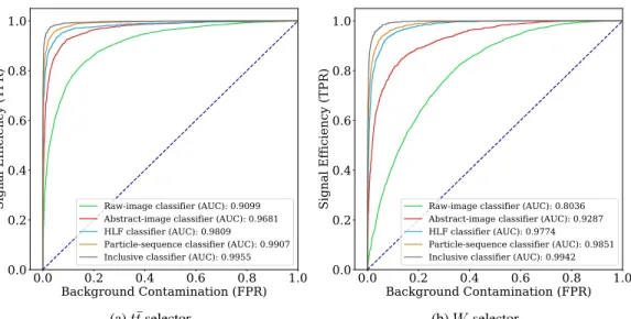
the corresponding receiver operating characteristic (ROC) curve. Fig. 5 shows the comparison of the ROC curves for five classifiers: the DenseNets based on raw images and abstract images, the GRU using the list of particles, the DNN using the HLFs, and the inclusive classifier using both the HLFs and the list of particles. Results for both att¯andW selectors are shown.

Acceptable results are obtained already with the raw-image classifier. On the other hand, the use of abstract images allows us to reach better performances. A further improvement is observed for those models not using an image-based representation of the event. The fact that the HLF selectors perform so well doesn’t come as a surprise, given a considerable amount of physics knowledge implicitly provided by the choice of the relevant features. On the other hand, the fact that the particle-sequence classifier reaches comparable performances to the HLF selector is remarkable, as is the further improvement observed by merging the two approaches in the inclusive classifier. In some sense, the GRU layer is gaining a good part of the physics intuition that motivated the choice of the HLF quantities, but not entirely. Fig. 6 shows the Pearson correlation coefficients between the GRU scores (ytt¯andyW) and the HLF quantities. As one would expect,yt¯texhibits a stronger correlation with

those features that quantify jet activity, as well as with the b-jet multiplicity. On the contrary,W events shows an anti-correlation with respect to jet quantities, since the production of associated jets inW events is much more penalized than fort¯tevents. As expected, both scores are anti-correlated to the isolation quantities, which takes larger values for non-isolated leptons.

The performance of each of the five classifiers is summarized in Tab. 1 in terms of false-positive rate (FPR) and trigger rate (TR) as a function of the true-positive rate (TPR). The best QCD rejection is

(8)

0.0

0.2

0.4

0.6

0.8

1.0 Background Contamination (FPR)

0.0

0.2

0.4

0.6

0.8

1.0 Signal Efficiency (TPR)

Raw-image classifier (AUC): 0.9099 Abstract-image classifier (AUC): 0.9681 HLF classifier (AUC): 0.9809

Particle-sequence classifier (AUC): 0.9907 Inclusive classifier (AUC): 0.9955

(a)t¯tselector

0.0

0.2

0.4

0.6

0.8

1.0 Background Contamination (FPR)

0.0

0.2

0.4

0.6

0.8

1.0 Signal Efficiency (TPR)

(b)Wselector

Figure 5: ROC curves for thet¯t(left) andW (right) selectors described in the paper.

ST E mis s T | mis s| M2 T njets nbjet s _pT _|| _|| ch arg e Ga mm aP FIs o Ne uP FIs o Ch PF Iso _isEle 0.4 0.2 0.0 0.2 0.4

Pearson correlation coefficient

ST E mis s T | mis s| M2 T njets nbjets p T _|| _|| ch arg e Ga mm aP FIs o Ne uP FIs o Ch PF Iso _isEle 0.4 0.2 0.0 0.2 0.4

Pearson correlation coefficient

Figure 6: Pearson correlation coefficients between theyt¯t(left) andyW (right) scores of the

Particle-sequence classifier and the 14 quantities of the HLF dataset.

obtained by the inclusive classifier, which can retain 99% of thet¯torW events with a false-positive rate of∼8%.

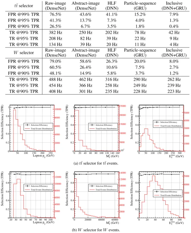
The trigger baseline selection we use in this study, looser than what is used nowadays in CMS, gives an overall trigger rate (i.e., summing electron and muon events) of∼690Hz, more than a factor two larger than what is currently allocated. Using the 99% working points of the two classifiers, one would reduce the overall rate to∼280Hz (counting the overlap between the two triggers). This would be comparable to what is currently allocated for these triggers, but with a looser selection, i.e., with a less severe bias on the offline analysis. In addition, the trigger efficiency (the TPR) is so large that the bias imposed on offline quantities is quite minimal. This is illustrated in Fig. 7, where the dependence of the TPR on the most relevant HLF quantities is shown. In our experience, any rule-based algorithm with the same target trigger rate would result in larger inefficiencies at small values of at least some of these quantities, e.g., the leptonpT. One should also consider that the

principle of a topology classifier could be generalized to other physics cases, as well as to other uses (e.g., labels for fast reprocessing or access to specific subsets of the triggered samples).

5 Impact on other topologies

While reducing the resource consumption of standard physics analyses is the main motivation behind this study, it is important to evaluate the impact of the proposed classifiers on other kind of topologies. For this purpose, we consider a handful of beyond-the-standard-model (BSM) scenarios, and we

(9)

Table 1: False positive rate (FPR) and trigger rate (TR) at different values of the true positive rate (TPR), for at¯t(top) andW selector. Rate values are estimated scaling the TPR and process-dependent FPR values by the acceptance and efficiency, assuming a leading-order (LO) production cross section and luminosity of 2×1034cm−2s−1. TR values should be taken only as suggestions of the actual rates, since the accuracy is limited by the use of LO cross sections and a parametric detector simulation.

t¯tselector Raw-image Abstract-image HLF Particle-sequence Inclusive

(DenseNet) (DenseNet) (DNN) (GRU) (DNN+GRU)

FPR @99% TPR 76.5% 43.6% 41.1% 15.2% 7.9% FPR @95% TPR 41.3% 13.7% 7.3% 4.0% 1.3% FPR @90% TPR 26.5% 6.7% 3.5% 1.8% 0.4% TR @99% TPR 382 Hz 250 Hz 202 Hz 78 Hz 42 Hz TR @95% TPR 208 Hz 82 Hz 39 Hz 22 Hz 9 Hz TR @90% TPR 134 Hz 39 Hz 20 Hz 11 Hz 4 Hz

W selector Raw-image Abstract-image HLF Particle-sequence Inclusive

FPR @99% TPR 79.0% 58.6% 26.3% 20.0% 8.0% FPR @95% TPR 60.5% 26.4% 10.6% 7.5% 2.7% FPR @90% TPR 48.1% 14.9% 5.8% 3.7% 1.2% TR @99% TPR 488 Hz 462 Hz 316 Hz 290 Hz 262 Hz TR @95% TPR 454 Hz 366 Hz 258 Hz 249 Hz 239 Hz TR @90% TPR 408 Hz 301 Hz 235 Hz 228 Hz 223 Hz 50 100 150 200 250 (GeV) T Lepton p 0 0.2 0.4 0.6 0.8 1 Selection Efficiency (TPR) Selection Efficiency Total Events Distribution

0 2000 4000 6000 8000 10000 0 20 40 60 80 100 120 140 160 3 10 × (GeV) 2 T M 0 0.2 0.4 0.6 0.8 1 Selection Efficiency (TPR) Selection Efficiency Total Events Distribution

0 5000 10000 15000 20000 25000 0 50 100 150 200 250 300 (GeV) miss T E 0 0.2 0.4 0.6 0.8 1 Selection Efficiency (TPR) Selection Efficiency Total Events Distribution

0 1000 2000 3000 4000 5000

(a)t¯tselector fortt¯events.

20 30 40 50 60 70 80 90 100 (GeV) T Lepton p 0 0.2 0.4 0.6 0.8 1 Selection Efficiency (TPR) Selection Efficiency Total Events Distribution

0 2000 4000 6000 8000 10000 12000 0 20000 40000 60000 (GeV) 2 T M 0 0.2 0.4 0.6 0.8 1 Selection Efficiency (TPR) Selection Efficiency Total Events Distribution

0 2000 4000 6000 8000 10000 12000 14000 0 20 40 60 80 100 (GeV) miss T E 0 0.2 0.4 0.6 0.8 1 Selection Efficiency (TPR) Selection Efficiency Total Events Distribution

0 1000 2000 3000 4000 5000

(b)W selector forWevents.

Figure 7: Selection efficiency using 99% TPR working point as functions of leptonpT,MT2, and

Emiss

T fort¯tandWevents.

compute the TPR as a function of the most relevant kinematic quantities, similar to what was done in Fig. 7 for the standard topologies.

(10)

20 40 60 80 100 120 140 160 180 200 (GeV) T Lepton p 0 0.2 0.4 0.6 0.8 1 Selection Efficiency (TPR) 0 500 1000 1500 2000 2500 selector t t W+jets selector OR selectors Total events

0 20000 40000 60000 80000 (GeV) 2 T M 0 0.2 0.4 0.6 0.8 1 Selection Efficiency (TPR) 0 2000 4000 6000 8000 10000 selector t t W+jets selector OR selectors Total events

0 50 100 150 200 250 (GeV) miss T E 0 0.2 0.4 0.6 0.8 1 Selection Efficiency (TPR) 0 500 1000 1500 2000 2500 selector t t W+jets selector OR selectors Total events

(a)A→H+W− 0 50 100 150 200 250 300 350 400 (GeV) T Lepton p 0 0.2 0.4 0.6 0.8 1 Selection Efficiency (TPR) 0 1000 2000 3000 selector t t W+jets selector OR selectors Total events

0 50 100 150 3 10 × (GeV) 2 T M 0 0.2 0.4 0.6 0.8 1 Selection Efficiency (TPR) 0 2000 4000 6000 8000 10000 12000 14000 selector t t W+jets selector OR selectors Total events

0 50 100 150 200 250 300 350 400 450 (GeV) miss T E 0 0.2 0.4 0.6 0.8 1 Selection Efficiency (TPR) 0 1000 2000 3000 selector t t W+jets selector OR selectors Total events

(b) High-massA→H+W− 0 100 200 300 400 500 600 (GeV) T Lepton p 0 0.2 0.4 0.6 0.8 1 Selection Efficiency (TPR) 0 1000 2000 3000 selector t t W+jets selector OR selectors Total events

0 20 40 60 80 100 3 10 × (GeV) 2 T M 0 0.2 0.4 0.6 0.8 1 Selection Efficiency (TPR) 0 5000 10000 15000 20000 selector t t W+jets selector OR selectors Total events

(c)A→4` 50 100 150 200 (GeV) T Lepton p 0 0.2 0.4 0.6 0.8 1 Selection Efficiency (TPR) 0 200 400 600 800 1000 1200 selector t t W+jets selector OR selectors Total events

0 50 100 150 3 10 × (GeV) 2 T M 0 0.2 0.4 0.6 0.8 1 Selection Efficiency (TPR) 0 2000 4000 6000 8000 selector t t W+jets selector OR selectors Total events

0 50 100 150 200 250 (GeV) miss T E 0 0.2 0.4 0.6 0.8 1 Selection Efficiency (TPR) 0 200 400 600 800 1000 1200 selector t t W+jets selector OR selectors Total events

(d)W0 0 100 200 300 400 500 600 (GeV) T Lepton p 0 0.2 0.4 0.6 0.8 1 Selection Efficiency (TPR) 0 1000 2000 3000 selector t t W+jets selector OR selectors Total events

0 20 40 60 80 100 3 10 × (GeV) 2 T M 0 0.2 0.4 0.6 0.8 1 Selection Efficiency (TPR) 0 2000 4000 6000 8000 10000 selector t t W+jets selector OR selectors Total events

(11)

We consider the following BSM processes:

• A →H+_W_{: a heavy Higgs boson}_A_{with mass 425 GeV decaying to a charged Higgs}

bosonH+of mass 325 GeV and aW−boson. TheH+then decays to aW+H0final state, whereH0_{is the 125 GeV Higgs boson, which we force to decay to a bottom quark-antiquark}

pair. This model, introduced in Ref. [20], generates a 2b2W topology similar to that given byt¯tevents.

• High-massA→H+W: a high-mass variation of the previous model, in which theAand

H+_{masses are set to 1025 GeV and 625 GeV, respectively.}

• A→4`: a light neutral scalar particleAwith mass 20 GeV, decaying to two neutral scalars of 5 GeV each, both decaying to muon pairs, for a total of four muons in the final state.

• W0resonance with mass 300 GeV, decaying inclusively withW-like couplings.

• Z0resonance with mass 600 GeV, decaying to a pair of electrons of muons. These events are filtered with the baseline selection described in Sect. 2.

For each of these models, we consider the inclusive classifier and apply the 99%-TPR thresholds on yt¯tandyW. We then consider the fraction of events passing at least one of the two selectors. Results

are shown in Fig. 8 for the most relevant kinematic quantities. While the individual selectors might show local inefficiencies, the combination of the two trigger paths is perfectly capable of retaining any event with features different from that of a QCD multijet event. In this respect, the logicalOR of our two exclusive topology classifiers is robust enough to also select a large spectrum of BSM topologies. On the other hand, one cannot guarantee that QCD-like topologies (e.g., a dark photon produced in jet showers and decaying to lepton pairs) would not be rejected, a limitation which also affects traditional inclusive trigger strategies.

6 Related work

Several classification algorithms have been studied in the context of LHC physics application, notably for jet tagging [21, 22, 23, 24, 25, 26, 27, 28] and event topology identification [20, 29, 11] using feed-forward neural networks, convolutional neural networks or physics-inspired architectures. Lists of particles have been used to define jet and event classifiers starting from a list of reconstructed particle momenta [30, 31, 32]. These studies typically consider data analysis as the main use case, focusing on small FPR selections. This is the main difference with respect to this study, which is more related to an optimization of the data-taking procedure.

7 Conclusions

We show how deep neural networks can be used to train topology classifiers for LHC collision events, which could be used as a cleanup filter to select or reject specific event topologies in a trigger system. We consider several network architectures, applied to different representations of the same collision datasets. The best results are obtained by combining a set of physics-motivated high-level features with the output of a GRU unit applied to a list of particle-level features. For the most difficult case, i.e., selecting raret¯tevents, we show how a trigger based on this concept would retain 99% of the tt¯events while reducing the FPR by as much as∼10times. We show that such a trigger would have a minimal impact on the main kinematic features of the event topologies under consideration. In addition, the logicORof thett¯andW selections would also catch a broad class of new-physics topologies, on which the classifiers were not trained. In view of the challenging trigger environment foreseen for the High-Luminosity LHC, it would be important to test this trigger strategy as a way to preserve a good experimental reach with a substantial reduction of computational resources. In this respect, we look forward to the LHC Run III as an opportunity to experiment this technique with real data.

8 Acknowledgments

This work is partially supported by a grant from the Swiss National Supercomputing Center (CSCS) under project ID d59. We thank CERN OpenLab for supporting DW during his internship at CERN.

(12)

We are grateful to Caltech and the Kavli Foundation for their support of undergraduate student research in cross-cutting areas of machine learning and domain sciences. Part of this work was conducted at "iBanks", the AI GPU cluster at Caltech. We acknowledge NVIDIA, SuperMicro and the Kavli Foundation for their support of "iBanks". This project is partially supported by the United States Department of Energy, Office of High Energy Physics Research under Caltech Contract No. de-sc0011925. This project has received funding from the European Research Council (ERC) under the European Union’s Horizon 2020 research and innovation program (grant agreement no772369).

References

[1] ATLASCollaboration, M. Aaboud et al.,Performance of the ATLAS Trigger System in 2015,

Eur. Phys. J.C77(2017), no. 5 317, [arXiv:1611.09661].

[2] W. Adam et al.,The CMS high level trigger,Eur. Phys. J.C46(2006) 605–667,

[hep-ex/0512077].

[3] Y. LeCun, B. E. Boser, J. S. Denker, et al.,Handwritten digit recognition with a

back-propagation network, inAdvances in Neural Information Processing Systems 2(D. S. Touretzky, ed.), pp. 396–404. Morgan-Kaufmann, 1990.

[4] S. Hochreiter and J. Schmidhuber,Long short-term memory,Neural Comput.9(Nov., 1997)

1735–1780.

[5] K. Cho, B. van Merrienboer, D. Bahdanau, and Y. Bengio,On the properties of neural machine translation: Encoder-decoder approaches,CoRRabs/1409.1259(2014) [arXiv:1409.1259]. [6] T. Sjöstrand, S. Ask, J. R. Christiansen, et al.,An Introduction to PYTHIA 8.2,Comput. Phys.

Commun.191(2015) 159–177, [arXiv:1410.3012].

[7] DELPHES 3Collaboration, J. de Favereau, C. Delaere, P. Demin, et al.,DELPHES 3, A

modular framework for fast simulation of a generic collider experiment,JHEP02(2014) 057,

[arXiv:1307.6346].

[8] D. Contardo, M. Klute, J. Mans, L. Silvestris, and J. Butler,Technical Proposal for the Phase-II Upgrade of the CMS Detector, .

[9] M. Cacciari, G. P. Salam, and G. Soyez,FastJet User Manual,Eur. Phys. J.C72(2012) 1896,

[arXiv:1111.6097].

[10] M. Cacciari, G. P. Salam, and G. Soyez,The anti-ktjet clustering algorithm,Journal of High

Energy Physics2008(2008), no. 04 063.

[11] C. F. Madrazo, I. H. Cacha, L. L. Iglesias, and J. M. de Lucas,Application of a Convolutional Neural Network for image classification to the analysis of collisions in High Energy Physics,

arXiv:1708.07034.

[12] A. Paszke, S. Gross, S. Chintala, et al.,Automatic differentiation in PyTorch, .

[13] R. Al-Rfou, G. Alain, A. Almahairi, et al.,Theano: A Python framework for fast computation of mathematical expressions,arXiv e-printsabs/1605.02688(May, 2016).

[14] D. P. Kingma and J. Ba,Adam: A Method for Stochastic Optimization,ArXiv e-prints(Dec.,

2014) [arXiv:1412.6980].

[15] D. Anderson, M. Spiropulu, and J.-R. Vlimant,An MPI-Based Python Framework for

Distributed Training with Keras,arXiv:1712.05878.

[16] F. Pedregosa, G. Varoquaux, A. Gramfort, et al.,Scikit-learn: Machine learning in Python,

Journal of Machine Learning Research12(2011) 2825–2830.

[17] V. Nair and G. E. Hinton,Rectified linear units improve restricted Boltzmann machines, in

Proceedings of ICML, vol. 27, pp. 807–814, 06, 2010.

[18] G. Huang, Z. Liu, L. van der Maaten, and K. Q. Weinberger,Densely connected convolutional networks, inProceedings of the IEEE Conference on Computer Vision and Pattern Recognition, 2017.

[19] S. Catani, Y. L. Dokshitzer, M. H. Seymour, and B. R. Webber,Longitudinally invariantKt

(13)

[20] P. Baldi, P. Sadowski, and D. Whiteson,Searching for exotic particles in high-energy physics with deep learning,Nature Communication5(07, 2014) 4308.

[21] L. de Oliveira, M. Kagan, L. Mackey, B. Nachman, and A. Schwartzman,Jet-images — deep

learning edition,JHEP07(2016) 069, [arXiv:1511.05190].

[22] D. Guest, J. Collado, P. Baldi, et al.,Jet Flavor Classification in High-Energy Physics with Deep Neural Networks,Phys. Rev.D94(2016), no. 11 112002, [arXiv:1607.08633]. [23] S. Macaluso and D. Shih,Pulling Out All the Tops with Computer Vision and Deep Learning,

arXiv:1803.00107.

[24] K. Datta and A. J. Larkoski,Novel Jet Observables from Machine Learning,

arXiv:1710.01305.

[25] A. Butter, G. Kasieczka, T. Plehn, and M. Russell,Deep-learned Top Tagging with a Lorentz Layer,arXiv:1707.08966.

[26] G. Kasieczka, T. Plehn, M. Russell, and T. Schell,Deep-learning Top Taggers or The End of

QCD?,JHEP05(2017) 006, [arXiv:1701.08784].

[27] P. T. Komiske, E. M. Metodiev, and M. D. Schwartz,Deep learning in color: towards

automated quark/gluon jet discrimination,JHEP01(2017) 110, [arXiv:1612.01551].

[28] A. Schwartzman, M. Kagan, L. Mackey, B. Nachman, and L. De Oliveira,Image Processing,

Computer Vision, and Deep Learning: new approaches to the analysis and physics interpretation of LHC events,J. Phys. Conf. Ser.762(2016), no. 1 012035.

[29] W. Bhimji, S. A. Farrell, T. Kurth, et al.,Deep Neural Networks for Physics Analysis on low-level whole-detector data at the LHC, in18th International Workshop on Advanced Computing and Analysis Techniques in Physics Research (ACAT 2017) Seattle, WA, USA, August 21-25, 2017, 2017.arXiv:1711.03573.

[30] G. Louppe, K. Cho, C. Becot, and K. Cranmer,QCD-aware recursive neural networks for jet

physics,arXiv:1702.00748.

[31] S. Egan, W. Fedorko, A. Lister, J. Pearkes, and C. Gay,Long Short-Term Memory (LSTM)

networks with jet constituents for boosted top tagging at the LHC,arXiv:1711.09059.

(14)

Appendix A

In this paper, we showed how one could use a topology classifier to keep the overall trigger rate under control while operating triggers with otherwise unsustainable loose selections. In this appendix we discuss how topology classifiers could be used to save resources for a pre-defined baseline trigger selection by rejecting events associated to unwanted topologies. In this case, the main goal is not to reduce the impact of the online selection. Instead, we focus on reducing resource consumption downstream for a given trigger selection.

To this purpose, we consider a copy of the dataset described in Sec. 2, obtained tightening thepT

threshold from 23 to 25 GeV and the isolation requirement fromISO< 0.45 toISO< 0.20. Doing so, the sample composition changes as follow: 7.5% QCD; 92%W; 0.5%t¯t. With such selections, the trigger acceptance rate would decrease from 690 Hz to 390 Hz, closer to what is currently allocated for these triggers in the CMS experiment.

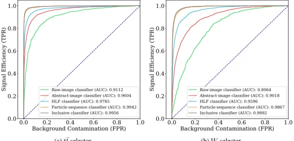
Following the procedure described in Sec. 3 and 4, we train the same topology classifiers on this dataset. The corresponding ROC curves are presented in Fig. 9 for att¯and aW selector.

0.0

0.2

0.4

0.6

0.8

1.0 Background Contamination (FPR)

0.0

0.2

0.4

0.6

0.8

1.0 Signal Efficiency (TPR)

(a)t¯tselector

0.0

0.2

0.4

0.6

0.8

1.0 Background Contamination (FPR)

0.0

0.2

0.4

0.6

0.8

1.0 Signal Efficiency (TPR)

(b)Wselector

Figure 9: ROC curves for thet¯t(left) andW (right) selectors described in the paper, trained on a dataset defined by a tighter baseline selection.

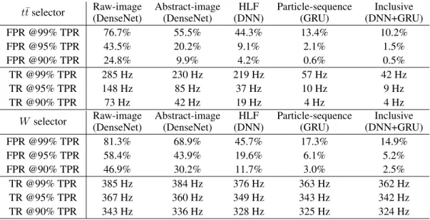
We then define a set of trigger filters applying a lower threshold to the normalized score of the classifier, choosing the threshold value that corresponds to a certain TPR value. The result is presented in Table 2, in terms of the FPR and the trigger rate.

The trigger baseline selection we use in this study, close to what is used nowadays in CMS for muons, gives an overall trigger rate (i.e., summing electron and muon events) of∼390 Hz (i.e., 190 Hz per lepton flavor). If one was willing to take (as an example) half theW events and all thet¯tevents, this number could be reduced to∼200Hz using the inclusive selectors presented in this study (taking into account the partial overlap between the two triggers). A more classic approach would consist in prescaling the isolated lepton triggers, i.e. randomly accepting half of the events. The effect on W events would be the same, but one would lose half of thet¯tevents while still writing 15 times more QCD thant¯tevents. In this respect, the strategy we propose would allow a more flexible and cost-effective strategy.

(15)

Table 2: False positive rate (FPR) and trigger rate (TR) corresponding to different values of the true positive rate (TPR), for at¯t(top) andW selector. Rate values are estimated scaling the TPR and process-dependent FPR values by the acceptance and efficiency, assuming a leading-order (LO) production cross section and luminosity of 2×1034_cm−2_s−1_{. TR values should be taken only as a}

loose indication of the actual rates, since the accuracy is limited by the use of LO cross sections and a parametric detector simulation.

t¯tselector Raw-image Abstract-image HLF Particle-sequence Inclusive

W selector Raw-image Abstract-image HLF Particle-sequence Inclusive