Quasi-pseudolikelihood in Markov network structure learning

(1)

Faculty of Science Department of Mathematics and Statistics Mikko Heikkilä

Quasi-Pseudolikelihood in Markov network structure learning Statistics

Master’s thesis October 2016 39 p.

Graphical models, undirected models, structure learning, pseudo-likelihood, quasi-likelihood Probabilistic graphical models are a versatile tool for doing statistical inference with complex mo-dels. The main impediment for their use, especially with more elaborate models, is the heavy computational cost incurred. The development of approximations that enable the use of graphical models in various tasks while requiring less computational resources is therefore an important area of research. In this thesis, we test one such recently proposed family of approximations, called quasi-pseudolikelihood (QPL).

Graphical models come in two main variants: directed models and undirected models, of which the latter are also called Markov networks or Markov random fields. Here we focus solely on the undi-rected case with continuous valued variables. The specific inference task the QPL approximations target is model structure learning, i.e. learning the model dependence structure from data. In the theoretical part of the thesis, we define the basic concepts that underpin the use of graphical models and derive the general QPL approximation. As a novel contribution, we show that one member of the QPL approximation family is not consistent in the general case: asymptotically, for this QPL version, there exists a case where the learned dependence structure does not converge to the true model structure.

In the empirical part of the thesis, we test two members of the QPL family on simulated datasets. We generate datasets from Ising models and Sherrington-Kirkpatrick models and try to learn them using QPL approximations. As a reference method, we use the well-established Graphical lasso (Glasso).

Based on our results, the tested QPL approximations work well with relatively sparse dependence structures, while the more densely connected models, especially with weaker interaction strengths, present challenges that call for further research.

Tiedekunta/Osasto — Fakultet/Sektion — Faculty Laitos — Institution — Department

Tekijä — Författare — Author

Työn nimi — Arbetets titel — Title

Oppiaine — Läroämne — Subject

Työn laji — Arbetets art — Level Aika — Datum — Month and year Sivumäärä — Sidoantal — Number of pages

Tiivistelmä — Referat — Abstract

Avainsanat — Nyckelord — Keywords

(2)

Quasi-Pseudolikelihood in Markov network structure

learning

Mikko Heikkil¨a

(3)

Introduction

Probabilistic graphical models offer a versatile way of presenting and utilizing complex probabilistic models in various tasks. Graphical models come in two main variants: directed and undirected ones. Both versions have attracted increasing interest during the last decades, that have seen a number of important theoretical and algorithmic developments. As a result, graphical models are becoming easier to use and steadily more useful in a wide range of applications.

Nevertheless, even though graphical models can be powerful tools for inference, they are naturally not without problems. The main impediment for their use is usually the heavy computational burden involved, especially with larger systems. One way to alleviate these problems is to find good approximations, that require less computations or enable circumventing some parts of the problem altogether.

Generally, it is possible to classify statistical inference problems into two main classes: parameter inference and structure learning. In this thesis we concentrate on the struc-ture learning problem in the special case of undirected graphical models. Our main interest lies in testing two versions of a new family of approximation methods, called quasi-pseudolikelihood (QPL), for scoring different model structures. Due to having an analytical expression, the evaluation of the QPL scorings is computationally efficient compared e.g. to a full Bayesian solution of the problem. In the theoretical part of this thesis, we present the basic theory needed for utilizing graphical models and then derive the QPL scoring. On the empirical side, we test two variants of the QPL scoring by applying them to structure learning problem in noisy Ising models and related noisy Sherrington-Kirkpatrick models. As a novel theoretical contribution, we show that one of the tested criterions is inconsistent in a specific case.

The most important general references used in this thesis are two articles, the first one presenting an approximation called marginal pseudo-likelihood [24] and the second one presenting the quasi-pseudolikelihood [9]. The marginal pseudo-likelihood article introduces many of the basic principles and ideas that the quasi-pseudolikelihood is then based on. As a general reference for graphical models, we use a book by Koller & Friedman [16], from which most of the basic definitions come from. For Ising and related models we refer to a book by MacKay [19].

(6)

The organization of the thesis is as follows. In chapter 2 we start by introducing undirected probabilistic graphical models as a tool for handling information in com-plex systems. In the subsections, we give formal definitions that underpin the use of undirected models for representation, inference, and structure learning.

In chapter 3, we present the general structure learning problem in graphical models. In the subsections we first present the standard Bayesian approach to structure learning and find that, in general, it cannot be used as such for structure learning in undirected graphical models because of the computational burden involved. We therefore move on to define an approximation called marginal pseudo-likelihood, that enables structure learning in a computationally more efficient manner for discrete random variables. This method is then extended in the last subsection to cover continuous random variables by defining the quasi-pseudolikelihood scoring.

In chapter 4, we move on to testing the quasi-pseudolikelihood on noisy Ising models, as well as on the related noisy Sherrington-Kirkpatrick models. We therefore first define the models and present some of their general properties. After this we introduce the Metropolis-Hastings algorithm used for generating the data. We continue on to present the general settings used in the testing as well as the test results.

(7)

Chapter 2

Graphical models

Graphical models have enjoyed increasing interest in the last few decades. Although the general idea of presenting interactions between variables as a graph has been traced back at least to J. Willard Gibbs in the beginning of the 20th century [11], graphical models started to garner more wide-spread recognition in Statistics from 1980 onwards, thanks to an article by Darroch, Lauritzen and Speed [7], where the authors combined the already well-established theory of Markov random fields and log-linear models, as well as some earlier work done on graphical models, to present graphical models as a separate class of models with several advantageous properties (see [16], [29]). Koller and Friedman credit the more widespread breakthrough of the graphical models towards the end of 1980s and the start of 1990s mainly to an influential textbook by Judea Pearl [23], and an article by Lauritzen and Spiegelhalter [17], which presented some key-ideas enabling more efficient inference using graphical models [16].

Arguably the most important aspect in considering graphical models is the equiva-lence of the dependence structure represented by a graph, and the factorization proper-ties of a joint distribution. When this equivalence holds, we can firstly use a graphical model for representation, i.e. we can present complex dependencies in a way that is, in general, a lot easier for humans to understand at a glance than a mathematical formula representation of the joint distribution.

Besides offering a convenient way to present dependencies in probabilistic systems for ease of understanding, this form of representation also enables us in many cases to define a joint distribution over the system with relative ease, utilizing the factorization properties of the joint distribution to avoid defining redundant parameters. With joint distributions having potentially dozens or hundreds of variables, this reduction in the number of parameters can be essential for the task to be manageable.

Secondly, in addition to the good representation properties, graphical models can also be used for carrying out statistical inference tasks, such as calculating posterior probabilities for events given information on some of the variables in the model. Since the inference algorithms developed for graphical models utilize the graph structure, and hence also the dependence structure, of the model in question, they tend to be faster than inference algorithms that work on the joint distribution as a whole.

(8)

Thirdly, graphical models framework can be used forlearning model structures. This enables a more data-driven approach, where human input defines some bounds on the possible models, and the final model or a set of models is learned algorithmically from the data at hand.

2.1 Basic definitions and notations

In this thesis we take some basic probability theory, such as random variables or den-sity functions, as granted without reviewing the actual definitions and results. All the necessary background information should be found in any basic textbook, such as [1].

Concerning notation, we usually write density functions and factors with a short-hand notation without explicitly noting the variables in question, e.g. for the joint density of some variables X we may write p(X) for the probability density or probability mass functionpX(X). This should not cause any misunderstandings, since the variables can always be identified from the context. With this clarificatory note, we can start defining concepts more central to the theme of graphical models.

Graphical models are based on mathematical graph theory, from where we have the following basic definition:

Definition 2.1.1(Graph). Let V be a set of nodes, and E be a set of edges,E ⊆V×V,

connecting the nodes. A graph is a collection G = (V, E). For an edge connecting variableVj to another variableVi, we write (j, i)∈E.

To use a graph to represent a joint distribution over a set of random variables X=

{X1, . . . , Xd}, we first interpret the nodes V ={1, . . . , d} to correspond to the indices of the variables. Henceforth, using this convention we usually refer to variables and nodes interchangeably. Depending on the way we define the edges, we get the two main types of graphical models: directed ones, usually called Bayesian networks (BNs), and undirected ones, which are also called Markov random fields (MRFs) or Markov networks (MNs). Since in this thesis the focus is on learning MN dependence structures, we do not consider BNs any further. For a more proper introduction, see e.g. [16].

For a MN, the edges connecting the variables are undirected, i.e. if (j, i) ∈ E ⇒

(i, j) ∈ E for all j 6= i. Variables connected by an edge are called neighbours, and the set of all neighbours is called aMarkov blanket, or more formally:

Definition 2.1.2 (Markov blanket). Let G = (V, E) be a graph corresponding to a Markov network, and letj∈V.A Markov blanket forjis the set of nodesmb(j) ={i∈ V|(j, i)∈E}.

Informally, in representing dependencies of a joint distribution with a graph, we would like to have some simple relationship between the dependencies and the edges. A preferable solution would be to have an edge in the graph between two variables whenever those variables are directly related, so that the edges would represent possible paths along which variables can influence one another. It turns out this intuitive idea is more or less achievable, depending on some assumptions concerning the distribution in

(9)

question. We return to this issue in defining the co-called Markov properties in chapter 2.3.

Besides Markov blankets, another useful concept when dealing with MN dependencies is a clique. A clique is simply a set of nodes, such that all nodes belonging to the same clique are connected by an edge in the graph. A maximal clique is a clique that cannot be enlarged any further by adding new nodes.

Definition 2.1.3 (Clique). Let G = (V, E) be a graph corresponding to a Markov network. A clique C is a set of nodes{i∈V|i∈C ⇒ (i, j)∈E for all j 6=i, j ∈C}. A clique C is called a maximal clique, if @i ∈V such that i6∈ C and (i, j) ∈ E for all

j∈C. We denote the set of maximal cliques in a graph Gby C(G).

We first assume that the variables Xj, j = 1, . . . , d are discrete, with an outcome spaceXj. We denote the cardinality of the outcome space as|Xj|=rj. This assumption is redefined later, when we move on to consider continuous variables defined on a closed interval [0,1]. For a subset of variables U ⊆V, we write XU ={Xj}j∈U. The outcome space of the subset is naturally a Cartesian product over the individual outcome spaces, i.e. XU =Q_j∈UXj, and the cardinality is the corresponding product over the individual cardinalities |X_U| =Q

j∈Urj. We denote an assignment to variables with a lower case letter, so thatxU is some specific joint assignment to variablesXU. Fornindependent, identically distributed (iid) joint observations, we generally writex= (x1, . . . ,xn), where

xk = (x1,k, . . . , xd,k). Throughout the thesis, we assume that the datasets are fully observed, meaning that there are no missing observations.

2.2 Parameterizing Markov networks

One important question that needs addressing, before we continue with the issues relating to the MN dependence structure, is how MNs can be parameterized. This issue turns out to be a lot thornier that might be expected. We therefore present the basic problem here only shortly and refer to [16] for a longer exposition.

Probably the first thing that comes to mind is to utilize conditional probability dis-tributions (CPDs) to parameterize MNs. However, since in MNs the influences between variables run both ways, there is no clear way to factorize the corresponding distribution into CPDs in such a way that the factorization respects the properties implied by the graph.

The standard answer to this conundrum is to use more general factors to represent the distribution. A factor is simply a mapping from the outcome space of the random variables to real numbers:

Definition 2.2.1 (Factor). Let X be a set of random variables. A function φ:X →_R

is called a factor. If the image of X under φis restricted to non-negative or to positive reals, then the factor is called a non-negative or a positive factor, respectively.

If not stated otherwise, henceforth we assume the factors to be non-negative. To utilize factors to represent distributions, we also need to have a suitable product rule, such as the one given in the following definition:

(10)

Definition 2.2.2 (Factor product). Let A, B, C be three disjoint sets of variables, and letφ1(A, B),φ2(B, C) be two factors. A factor productφ1×φ2 is defined to be a factor

ψ:X_A,B,C →_R,ψ(A, B, C) =φ1(A, B)·φ2(B, C).

A noteworthy point in this definition is that the factor product matches the common part of the individual factors.

It is immediately clear that joint distributions and CPDs are both special cases of general factors. Using the general factor definition we can define a Gibbs distribution, which is an undirected parameterization for a distribution. As such it forms a suitable link to the MN representation.

Definition 2.2.3(Gibbs distribution). A distributionpΦ is aGibbs distribution

param-eterized by a set of factors Φ ={φ1(D1), . . . , φK(DK)}, if it is defined as follows:

pΦ(X1, . . . , Xd) =1/Z·p˜Φ(X1, . . . , Xd), where ˜

pΦ(X1, . . . , Xd) =φ1(D1)×φ2(D2)× · · · ×φm(Dm)

is an unnormalized measure and

Z = X

X1,...,Xd ˜

pΦ(X1, . . . , Xd).

The normalizing constantZ is often called apartition functionfollowing the terminology used in statistical physics, since it is a function of the model parameters.

The key idea in unifying the Gibbs distribution formulation and a MN representation is to make a connection between factors in a distribution and cliques in a graph: a factor in the Gibbs distribution corresponds to a clique in the graph. This factorization prop-erty eventually allows us to formulate the Markov properties that define the dependence structure implied by a MN.

Definition 2.2.4 (Factorization). A distribution pΦ, Φ = {φ1(D1), . . . , φK(DK)}, is said to factorize over a Markov network, if each Dk, k = 1, . . . , K is a clique in the graph.

Factors corresponding to cliques that are used to parameterize a MN are often called

clique potentials.

It is worth noting that this factorization property generally does not lead to a unique parameterization, quite the contrary: if we have a parameterization with clique potentials that do not correspond to maximal cliques, then we can always find a new parameter-ization in terms of maximal clique potentials simply by taking factor products over all the factors that are encompassed in the same maximal clique.

This non-uniqueness of parameterizations is not limited to the case of maximal clique potentials but is a more fundamental issue: there is no single optimal parameterization for all purposes. Instead, what constitutes a useful parameterization depends on the situation. Different parameterizations can be loosely characterized by their granularity,

(11)

in other words by the level of detail they purpose to express. A parameterization more fine-grained than the one used in this thesis (that operates on the level of Markov blankets) can be expressed, for example, using factor graphs or log-linear models.

The key issue in choosing between the different parameterizations is the purpose of the representation. However, since this issue is not essential to this thesis, we stop here and proceed to treat the more central theme of dependence structures.

2.3 Markov properties

In order to meaningfully represent a joint distribution of some variables X with a graph, we need to know if the graph can properly capture all the intricacies inherent in the joint distribution and, on the other hand, if the graph can have some properties not satisfied by the distribution. The most basic properties we are now interested in are the conditional independencies between sets of variables. In the following, we write conditional independence statements as

XA⊥⊥XB|XC,

meaning that variables XA are conditionally independent of XB given XC, or equiva-lently that p(XA|XB, XC) =p(XA|XC).

With a joint distribution, as is evident from the notation above, conditional inde-pendence means that the distribution function factorizes into separate products, i.e. if

XA⊥⊥XB|XC, then

p(XA, XB|XC) =p(XA|XC)p(XB|XC).

With MNs, we want to express the conditional independence statements with a graph structure. In order to do this, we need to define the so-called Markov properties, that articulate the conditional independencies we can encode with MNs.

Before giving the definitions, we need some auxiliary concepts, namely paths and sep-arations. Intuitively, a path is an unbroken succession of edges between some variables, that allows a variable to have an influence on the non-neighbouring variables along the path. Since observing a variable fixes its value, it also blocks any influence from flowing through the observed variable. This means that we have to distinguish the so-called active paths that connect variables from all possible paths. Variables are separated if there is no active path connecting them.

Definition 2.3.1(Path). LetG= (V, E) be a graph corresponding to a MN. The nodes

Vp = (V1, . . . , Vj) form apath in G, if (i, i+ 1)∈E for all i, i+ 1∈Vp.

Definition 2.3.2 (Active path). Let G = (V, E) be a graph corresponding to a MN,

Vp = (V1, . . . , Vj) a path in G, and let Z ⊆V be a set of observed variables. The path

Vp is called active given Z, if for all i∈Vp,i6∈Z.

Definition 2.3.3 (Separation). Let V be the set of variables in a MN, A, B, C ⊂ V. SetCseparates Aand B, if there is no active path between nodesi∈A, j ∈B given C.

(12)

Using these concepts, we can properly characterise the dependencies implied by MNs. There are three different Markov properties that a given graph can satisfy: pairwise, local, and global. The pairwise Markov property states that any two variables that are not neighbours are conditionally independent of each other given all the other nodes in the graph. The local Markov property says that a variable is conditionally independent of any non-neighbouring node given its Markov blanket. Finally, the global Markov property affirms that given two distinct sets of variables, if we can find a separating set of variables between them, then any pairs of variables in the original sets are conditionally independent given the separating set.

The following three definitions formulate the different Markov properties for MNs:

Definition 2.3.4 (Pairwise Markov property). Xj ⊥⊥Xi|XV\{j,i} for allj, i∈V, such

that (j, i)∈/ E.

Definition 2.3.5 (Local Markov property). Xj ⊥⊥XV\{mb(j)∪j}|Xmb(j), for all j∈V.

Definition 2.3.6 (Global Markov property). XA ⊥⊥ XB| XC, for all disjoint subsets (A, B, C) of V, such thatC separatesAfrom B.

The structure scoring functions derived in the following chapters are based on the local Markov property, i.e. they utilize the Markov blankets for learning the dependence structure of the model in question. Generally speaking, the different Markov properties are not equivalent. However, it can be shown that in the special case of positive joint distributions, all the Markov properties are in fact equivalent (see e.g. [16]). We assume from now on, that the joint distributions are positive, unless noted otherwise.

We can also ask, are the dependence structures of a given joint distribution and some MN equivalent, i.e. do they encode the same conditional independencies. It is evident that in general, we can have a joint distribution with conditional independencies that we cannot represent with a MN (e.g. Bayesian networks provide counter-examples galore, see e.g. [16] for specific examples) and vice versa. A graph is called a perfect map for the joint distribution if it satisfies all the conditional independence statements encoded by the distribution and satisfies no conditional independence statements besides these. Similarly, if a graph is a perfect map for a distribution, then the distribution is called

faithful to the graph. For the rest of the thesis we assume that the graphs are perfect maps, unless otherwise noted.

Having defined the dependence structures associated with MNs and their relations with the corresponding properties of joint distributions, we continue next to treat the structure learning problem in MNs.

(13)

Chapter 3

Structure learning problem

Fully learning a statistical model usually involves two main components: structure learn-ing and parameter estimation, where by structure learnlearn-ing we mean learnlearn-ing the depen-dencies between the variables in a given model. In this thesis we are only interested in learning the model structure. Naturally, in real world problems it is not uncommon to encounter the two jointly: when doing statistical inference, we generally cannot depend on having a nice problem with a dependence structure fully known in advance, and when doing structure learning, we would in many cases also be interested in learning the pa-rameters of the model. However, in both of these cases the complete problem can be solved in pieces, by first learning the model structure and then inferring the parameters given the structure learned.

In general, structure learning methods can be roughly divided into constraint-based and score-based methods. Constraint-based methods aim to recover the model structure by utilizing tests of independencies between variables, whereas score-based methods use an objective function to evaluate the different structures. The latter approach then also requires solving an optimization problem to find the structure that maximizes (or minimizes) the objective function used. Since constraint-based methods typically are more sensitive to mistakes made with individual edges and tend to require more data to achieve correct results, the choice between different methods usually involves a trade-off between accuracy of the discovered structure and computational burden [16],[24].

3.1 Bayesian solution to structure learning

The heart of Bayesian inference is contained in the Bayes’ formula, which can be written as

p(φ|y) = R p(y|φ)p(φ)

φp(y|φ)p(φ)dφ

∝p(y|φ)p(φ), (3.1) whereφis some random quantity we like to make inferences on,yrefers to some quantity the inference is based on (typically observed data),p(y|φ) is the likelihood function, and

(14)

not interested in the normalizing constant R_φp(y|φ)p(φ)dφ and will therefore use just the unnormalized form. A thorough formulation of Bayesian theory can be found, for example, in [3].

Ideally, a full Bayesian solution to structure learning involves defining prior and likelihood functions for different graph structures, and then using Bayes’ formula (3.1) to arrive at the posterior distribution. For a graphG, this results in a marginal posterior probability p(G|x)∝p(x|G)p(G) = Z θG p(x|θG, G)p(θG|G)p(G)dθG (3.2) = Z θG { n Y k=1 p(xk|θG, G)}p(θG|G)p(G)dθG, (3.3)

where the key term for structure learning, that can be termed evidence, is

p(x|G) =

Z

θG

p(x|θG, G)p(θG|G)dθG. (3.4) The evidence effectively measures how likely the observed dataset is under the as-sumed modelG. Alas, (3.3) cannot usually be solved analytically without making some strict assumptions on the graphG. This might not be a huge problem, given that there are advanced methods like different flavours of Markov Chain Monte Carlo (MCMC) for evaluating just such integrals, if not for the size of the problem. Since there are 2(d2)

possible model structures, using current techniques with non-trivial sized problems, it may simply be infeasible to utilize the full marginal posterior distribution as such.

3.2 Marginal pseudo-likelihood

One viable alternative to the use of the true evidence of a model, defined in (3.4), is to use some approximation that leads to an analytically solvable expression. One such formulation, called marginal pseudo-likelihood was derived by Pensar & al. [24]. Assuming the model consists of discrete variablesX ={X1, . . . , Xd}, the MPL score for a graph is defined as d Y j=1 qj Y l=1 Γ(αjl) Γ(njl+αjl) rj Y i=1 Γ(nijl+αijl) Γ(αijl) , (3.5)

where d, qj and rj refer to the number of variables in the graph, the states of the MB for variable j, and the states of variable j, respectively. In addition,nijl is the number of times the configuration {Xj = x(i), Xmb(j) = x

(l)

mb(j)} appears in the data. Using a

similar notation, αijl >0 ∀ i, j, l refers to the corresponding prior parameters. Finally, by definition we havenjl=Pinijlandαjl=Piαijl. In this thesis, we use a prior given by

(15)

αijl = N |X | · |X_mb₍_j₎| = N rj ·qj , (3.6)

where the parameterN is the so-called equivalent sample size that adjusts the strength of the prior.

In the rest of this section we derive the MPL approximation and discuss the assump-tions needed to arrive at the analytical solution given in (3.5).

Starting from the true evidence (3.4), as a first step we replace the likelihood func-tion p(x|θG, G) = p(θG;x) with a pseudo-likelihood function. The pseudo-likelihood, originally introduced by Besag [4], uses a product of conditional likelihood functions to approximate the true likelihood. For a graphGthe pseudo-likelihood can be written as

pl(θG;x) = n Y k=1 d Y j=1 p(xj,k|xV\j,k, θG) = n Y k=1 d Y j=1 p(xj,k|xmb(j,k), θG), (3.7) where the first equality is by definition and the second one follows from the local Markov property for MNs (definition 2.3.5). Here mb(j, k) refers to the kth observation of the variables in mb(j). Replacing the true likelihood with the pseudo-likelihood effectively breaks the two-way interactions encoded by the edges in MNs locally into one-way in-fluences.

As an intermediary step in deriving the marginal pseudo-likelihood, we parameterize the conditional probabilities in the pseudo-likelihood (3.7) as

θijl:=p(Xj =xj(i)|Xmb(j)=x (l) mb(j)); θijl>0, rj X i=1 θijl = 1,

wherei= 1, . . . , rj,rj =|Xj|,l= 1, . . . , qj,qj =|mb(Xj)|=Q_i∈mb(j)ri. The indicesi, l

reference the configurations of the variable and its Markov blanket, respectively. Denote the counts of different configurations in the data as

nijl = n X k=1 I{(Xj,k, Xmb(j,k)) = (x (i) j,k,x (l) mb(j,k))}, and njl= rj X i=1 nijl, (3.8)

where I{?} is an indicator function. Using the above notation, the pseudo-likelihood (3.7) can be written as pl(θG;x) = d Y j=1 qj Y l=1 rj Y i=1 θn_ijlijl. (3.9)

In order to reach an analytical solution, we still need to define a prior distribution that factorizes in a way that fits in with the pseudo-likelihood formulation (3.9).

(16)

Defining sets of parameters by θjl=∪ rj i=1{θijl}, θj =∪ qj l=1{θjl}, θG=∪ d j=1{θj}, (3.10) we need a prior that factorizes as

f(θG) = d Y j=1 f(θj) = d Y j=1 qj Y l=1 f(θjl), (3.11)

which implies that θj ⊥⊥ θj0 if j 6= j0 (global parameter independence), and θ_jl ⊥⊥ θjl0 if jl 6= jl0 (local parameter independence). This factorization together with some

distributional assumptions leads to an analytical solution, as shown later.

This kind of prior formulation was presented by Heckerman & al. [14] for Bayesian networks, and consequently adapted by Pensar & al. [24] for MPL scoring prior. How-ever, assuming this prior produces a problem with MNs. With Bayesian networks, the assumptions of global and local parameter independencies can be reasonable ones, al-though not always [14]. In contrast, with a MN these assumptions directly violate the internal consistency of the MN, which has to be taken into account later on. Never-theless, the factorization is a necessary property if we want to arrive at an analytical formulation.

A third important assumption concerns the prior distributions of the parameter sets, which are assumed to follow a Dirichlet-distribution, i.e. we assume that

θjl ∼Dirichlet(α1jl, . . . , αrjjl), for allj, l, (3.12) whereα1jl, . . . , αrjjl are hyperparameters, which means that the functional form of the prior (3.11) is f(θG) = d Y j=1 qj Y l=1 f(θjl) = d Y j=1 qj Y l=1 Γ(Prj i=1αijl) Qrj i=1Γ(αijl) rj Y i=1 θαijl−1 ijl . (3.13)

This assumption is necessary, since the Dirichlet family of distributions is the conjugate family for a likelihood that follows a multinomial distribution. Following the earlier notation, we writeαjl=Pr_i₌₁j αijl.

Combining all the above assumptions, we can finally derive an analytical solution for the marginalization over the parameter values in the evidence (3.4), using standard Bayesian calculations (see e.g. [3]) presented here for convenience:

(17)

ˆ p(x|G) = Z θG pl(θG;x)·f(θG)dθG (3.14) = Z θG { d Y j=1 qj Y l=1 rj Y i=1 θnijl ijl } · { d Y j=1 qj Y l=1 f(θjl)}dθG (3.15) = Z θG d Y j=1 qj Y l=1 { rj Y i=1 θnijl ijl } · Γ(Prj i=1αijl) Qrj i=1Γ(αijl) rj Y i=1 θαijl−1 ijl dθG (3.16) = d Y j=1 qj Y l=1 Γ(Prj i=1αijl) Qrj i=1Γ(αijl) Z θjl rj Y i=1 θnijl+αijl−1 ijl dθjl (3.17) = d Y j=1 qj Y l=1 Γ(αjl) Qrj i=1Γ(αijl) Qrj i=1Γ(nijl+αijl) Γ(Prj i=1nijl+αijl) (3.18) = d Y j=1 qj Y l=1 Γ(αjl) Γ(njl+αjl) rj Y i=1 Γ(nijl+αijl) Γ(αijl) , (3.19)

where the integral in (3.17) can be readily calculated analytically by noting that it corresponds to a kernel of another Dirichlet distribution. Here we use the hat notation to differentiate the MPL score from the true marginal posterior, i.e. we write ˆp(x|G) instead of the true evidence (3.4).

To actually evaluate any concrete models in light of some given data, we also have to give values to the hyperparameters αijl. Pensar & al. [24] utilize a tweeked version of a prior originally introduced by Buntine [5] for Bayesian networks. This is just the prior given before in (3.6). The main motivation for using this type of prior is that, following [24], we are aiming at a more data-driven approach, where we do not favour any particular graph structure over any other. In other words we want to give equal weights to all parameters {θ1jl, . . . , θrjjl}.

One important question concerns the sensitivity of the results to this choice of pa-rameter value. Silander & al. [27] have demonstrated that the maximum a posteriori (MAP) results in structure learning using a so-called BDeu scoring can be sensitive to the equivalent sample size parameter value setting. Since MPL scoring is quite similar to the BDeu, it is expected to have similar properties, including the sensitivity to the prior equivalent sample size settings.

3.3 Quasi-pseudolikelihood

Hitherto we have assumed that the nodes V correspond to discrete random variables. Indeed, for Markov networks with continuous data there currently seems to exist pre-cious few options for efficient structure learning. The well-established methods typically assume the data to follow a multivariate Gaussian distribution, which obviously can be

(18)

a problematic assumption. The reason for this scarcity of methods is also evident: the likelihood function, which is the most natural choice for a scoring function, generally leads to intractable expressions.

Quasi-PseudoLikelihood (QPL) scoring is based on the same ideas as the MPL scoring introduced in the previous section 3.2, but this time the data is assumed to be continuous. The actual formulation of the QPL was done by Dikmen [9] based on the ideas presented in [20].

In the next two sections we first define the QPL scoring and discuss its derivation, and then review its computational complexity and the optimization needed in order to find top-scoring graph structures.

3.3.1 Definition and derivation of the QPL scoring

As with the MPL scoring in the previous chapter, we start by defining the QPL scoring and then derive the approximation and discuss the assumptions mostly towards the end of this subsection.

Assume our true data-generating model consists of unobserved binary random vari-ablesX={X1, . . . , Xd}. In addition, for eachXj we have an unobserved noise variable

j ∈[0,1] s.t. j ⊥⊥XA, B, whereA⊆ {1, . . . , d}, B⊆ {1, . . . , d} \j. Our observed variables Y ={Y1, . . . , Yd} are then given by

Yj =|Xj−j|, j = 1, . . . , d. (3.20)

In terms of graph structures, this means that for each binary variable in the original model, both the noise node and the binary node are connected to the new observed variable with a directed edge. In other words, we convert the original undirected binary model into a new noisy model, which includes both undirected and directed edges.

The QPL scoring is now defined as

˜ p(y|G) = d Y j=1 qj Y l=1 Γ(αjl) Γ(sjl+αjl) 1 Y i=0 Γ(sijl+αijl) Γ(αijl) , (3.21)

wheredandqj refer to the number of variables in the graph, and the states of the MB for variable j, in that order. We also have a prior similar to (3.5) given by αijl >0, αjl =

P

iαijl. The sijl and sjl terms that correspond to the counts in the discrete version (3.5) can be interpreted as fuzzy counts. They are defined in terms of sample-specific

responsibilities as sijl= n X k=1 sijlk, sjl= n X k=1 sjlk. (3.22)

(19)

Following [9], we define two different versions for the responsibilities leading to two distinct QPL scorings, termed QPL1 and QPL2. For QPL1, for variablejwith a MB of sizeNj the responsibility for thekth sample and configuration (i, l1, . . . , lNj) is given by

sijl1...l_Njk= (1− |i−yj,k|) Nj Y m=1 (1− |lm−ymb(j,m,k)|) (3.23) = (2iyj,k−yj,k−i+ 1) Nj Y m=1 (2lmymb(j,m,k)−ymb(j,m,k)−lm+ 1), (3.24) where, deviating from previous notation, we have written the variables in the MB ex-plicitly. The notation mb(j, m, k) refers to the kth observation for the mth variable in the MB mb(j). The responsibility for sjlk can be calculated from the same expression (3.24) by simply omitting the first factor that containsifrom the product.

For QPL2, the responsibility for the kth sample and configuration (i∗, l∗₁, . . . , l∗_N

j), (i∗, l₁∗, . . . , l∗_N_j) = arg min i,l1,...,l_Nj {|i−yj,k|+ Nj X m=1 |lm−ymb(j,m,k)|}, (3.25) is given by si∗_jl∗ 1...l∗_Njk= Nj + 1− |i∗−yj,k| −P Nj m=1|l∗m−ymb(j,m,k)| Nj + 1 . (3.26)

For all other configurations, the QPL2 responsibility is defined to be zero. For the respon-sibilitysjlk, we make simple modifications to (3.25) and (3.26) to get the corresponding expressions (l∗₁, . . . , l_N∗_j) = arg min l1,...,l_Nj { Nj X m=1 |lm−ymb(j,m,k)|}, (3.27) sjl₁∗...l_Nj∗ k= Nj−P Nj m=1|lm∗ −ymb(j,m,k)| Nj , (3.28)

and the responsibilities for all the other configurations are zeros.

In the rest of this section we derive the QPL approximation and discuss the various assumptions and some implications of the definitions. Most of the discussion presented in section 3.2 in deriving the MPL formulation is also relevant here, since MPL and QPL are very closely related, but we do not repeat it here.

We start the derivation by assuming that Xj ∈ {0,1}, j = 1, . . . , d. Since this is a stricter assumption than the general discreteness assumed in the previous chapters, the

(20)

MPL score formulation given in (3.5) remains valid. The basic idea is then to extend MPL by utilizing an approximation to quasi-likelihood functions.

Quasi-likelihood functions were originally introduced by Wedderburn [28] to allow for parameter estimation with generalized linear models in situations, where the true distribution of the response variable is unknown.

More verbosely, the basic idea with the quasi-likelihood is to relax the assumptions we need to make in order to model a dataset. The usual way to model some datapoints is to specify a likelihood function, which is then used to make inferences. However, this requires us to define the complete distribution of the data. Instead, with quasi-likelihood we only specify the relation between the mean and the variance. With some assumptions, we can make inferences about various interesting quantities such as regression coefficients using the quasi-likelihood function. The reason this works is that the quasi-likelihood is defined so as to share some basic properties with the common likelihood function (see e.g. [21]).

Denote the response variable by Y, E(Y) =µ, a dispersion parameter by σ2, and a variance function by V(?). Assuming the variance to have the form

Var(Y) =σ2V(µ),

the quasi-likelihood function is now defined as

Q(µ|y) =

Z

µ

y−t

σ2_V₍_t₎dt+g(y), (3.29)

whereg(y) is some function that does not depend on the model parameters. As shown in [28], the quasi-likelihood function has properties analogous to a standard likelihood function with respect to µ, and in the special case of one-parameter exponential family models, the quasi-likelihood is actually identical to the standard likelihood.

Marttinen & al. [20] used a quasi-likelihood approach in a fuzzy clustering problem, deriving a scoring function with a closed-form solution for the marginals in question. Using the same idea, Dikmen [9] defined a quasi-likelihood-based scoring method for MN structure learning. We present here the basic idea behind the QPL approximation and refer to [20] for a more thorough, information theoretic justification for the original approximation.

For a single binary observation of the variable Xj, the marginal density is given by the Bernoulli distribution. Parameterizing the distribution by µ we have the standard log-likelihood given by

logp(Xj =xj) =xjlogµ+ (1−xj) log(1−µ), xj ∈ {0,1}. (3.30) We would like to have a similar equation for a continuous-valued variableYj ∈[0,1]. As-suming that the variance functionV(?) in (3.29) has a similar form as the corresponding Bernoulli case, i.e. assuming that

(21)

and calculating the integral in (3.29) without the constant terms we get Q(µ|yj) = Z µ yj−t t(1−t)dt (3.32) =−yjlog( 1−µ µ ) + log(1−µ) (3.33) =yjlog(µ) + (1−yj) log(1−µ), (3.34) which clearly is not a proper likelihood function, but is nevertheless very similar to the Bernoulli log-likelihood (3.30). This is the basic solution used in [20], which is then developed further by including theσ2 term that is interpreted as measuring the amount of information in the observationyj.

In our case however, we need to consider the conditional densities instead of the marginal ones. Starting therefore again with a single binary variable Xj, we can write the full conditional distribution as

p(Xj|Xmb(j), θG, G) = p(Xj, Xmb(j)|θG, G) p(Xmb(j)|θG, G) = Q i Q lθ nijl ijl P Xj Q i Q lθ nijl ijl , (3.35)

where nijl are the counts over indicator functions as defined in (3.8). Replacing the binary variables with continuous ones, we could write the full conditional in a similar fashion as p(Yj|Ymb(j), θG, G) = Q i Q lθ sijl ijl R Q i Q lθ sijl ijl dYj , (3.36)

where sijl are the fuzzy counts, i.e. sums over some responsibilities. In other words, the individual responsibilities measure how similar the continuous variables are to the binary ones. This idea is somewhat similar to the information content tuned by σ2 in [20]. The integral in (3.36) complicates things, since it cannot be evaluated analytically. To overcome this problem, we have to make an approximation, i.e. we simply drop the normalizing constant and use the resulting terms

˜ p(Yj|Ymb(j), θG, G) = qj Y l=1 1 Y i=0 θs_ijlijl (3.37)

in the pseudo-likelihood defined in (3.7). This mean that QPL does not use a proper quasi-likelihood function but an approximation motivated by the quasi-likelihood ap-proach. To evaluate how much information this approximation loses, we need to test the method on various models.

With the fuzzy counts defined by (3.22), we can repeat the arguments and assump-tions given in the previous section to arrive at the analytical solution given in (3.21), that is very similar to the MPL scoring given in (3.5).

(22)

As has already been made evident, different definitions for the responsibilities lead to different QPL scorings, i.e. we should regard QPL as a family of related scoring methods.

A potential problem with the QPL1 responsibility defined in (3.24) is that it might re-sult in small fuzzy counts for relevant configurations especially in higher dimensions, since nothing constrains the normalizing constant dropped in (3.37) from being far from 1. In contrast, the QPL2 score first identifies the orthant the vector (yj,k, ymb(j,1,k), . . . , ymb(j,Nj,k)) belongs to by evaluating Manhattan distances as in (3.25). We then give positive re-sponsibility only to this closest configuration and set all other configurations to zero. The idea is that in this case, the normalizing constant that we drop in (3.37) is closer to or equal to one, so that omitting it has less effect on the final score.

One drawback in the QPL2 scoring definition is that by giving non-zero weight only to the single responsibility, we lose the property P

isijl = sjl∀j, l that can be used to evaluate the asymptotic properties of the fuzzy counts, as is done in appendix A.

We noted earlier in section 3.2 that the prior value is expected to have a notable influence on the MPL scoring. Since we use the same prior in the QPL formulation, it is also expected to have an influence on the QPL results.

One important theoretical property for estimators in general is consistency, which in this case guarantees that given enough observations, we are bound to identify the correct graph structure. Unfortunately, one novel contribution of this thesis is to show that there exists a case where QPL1 method is inconsistent, i.e. it is not consistent in a general case. In many cases, consistency could still be hoped for by restricting the possible graph structures to be e.g. chordal (meaning that there are no chordless cycles of length 4 or greater in the graph) or bipartite (meaning that the nodes in the graph can be clustered into two sets s.t. there are no edges connecting nodes in the same cluster). In the case of QPL1 however, the example constructed uses three vertices in a string, which means that the example also shows that QPL1 is not generally consistent even if the possible graph structures are quite strictly limited, e.g. to chordal or bipartite graphs. The proof can be found from appendix A. For QPL2 the consistency is still an open question.

3.3.2 Computational complexity and optimization

The MPL and QPL scorings derived in 3.2 and 3.3.1 define objective functions that can be used to evaluate different graph structures. The computational complexities of the MPL (covered in [24]) and QPL scorings are similar. With QPL scoring (3.21), using logarithms to avoid computational problems, to evaluate one graph structure we need to calculate the sum

d X j=1 qj X l=1 {log Γ(αjl)−log Γ(sjl+αjl) + 1 X i=0

(23)

which contains Pd

j=1(qj(2 + 2·2)) =

Pd

j=16qj terms. The number of variables d is

obviously constant for a given graph, but the number of different Markov blanket con-figurationsqj goes up exponentially with the size of the blanket.

Unlike with the MPL scoring, which can be implemented in a non-naive way to avoid at least part of the computations by only evaluating the blankets for which the configuration is also represented in the data, depending on the responsibility used the QPL scoring algorithm may actually need to evaluate all the possible Markov blanket configurations, since the fuzzy counts generally might not be zero for any configuration. As with the MPL scoring, the variable-wise decomposition of QPL makes it suitable for quick evaluation of local changes in a graph. Given two graphs G1 = (V, E1) and

G2= (V, E2), their log-QPL-ratio can be calculated by

logK(G1, G2) = log ˜p(y|G1)−log ˜p(y|G2), (3.39)

which could be interpreted as a kind of QP-Bayes factor. Assuming that the two graphs differ from each other by a single edge between, say, nodes i and i0, because of the decomposition properties of the QPL, equation (3.39) can be further modified by getting rid of some unnecessary terms. Since the single differing edge only affects the two Markov blankets mb(i) and mb(i0), removing the terms that cancel each other leads to

log K(G1, G2) = log ˜pi(y|G1) + log ˜pi0(y|G₁)−log ˜p_i(y|G₂)−log ˜p_i0(y|G₂), (3.40)

where e.g. ˜pi0 refers to the log-QPL score (3.38) with the indexj set to i0.

Despite the fact that the QPL scoring is given by a relatively simple formula, this still leaves us with a non-trivial optimization problem. The reason for this is the possible number of different graph structures, which goes up exponentially with the number of nodes in the graph. Even for moderate sized problems there are still too many possible structures for the problem to be manageable by brute computational force.

Therefore, instead of simply enumerating all the possible scorings and choosing the winner, we utilize the optimization algorithm described in [24]. We give here a shorter formulation elucidating the basic problem and the ideas ideas used for tackling it, and refer to the aforementioned article and the references therein for a more specific descrip-tion.

The basic optimization problem can be formulated as

arg max

G∈G log ˜p(y|G) + log p(G), (3.41)

where G is the set of all possible graph structures and p(G) is the prior distribution (see equation 3.3). Assuming the prior is uniform over all the possible structures, we drop it in the following expressions. The same ideas would also work with a suitable non-uniform prior with some corrections to the formulas. Since the model dependence structure is uniquely specified by the collection of Markov blanketsmb(G) ={mb(j)}d

(24)

(see Section 2.3 on Markov properties), we can write equation (3.41) equivalently using Markov blankets as arg max_mb₍_G₎∈×j∈VP(V\j) d X j=1 log ˜p(yj|ymb(j)) (3.42)

with the constraint that i ∈ mb(j) ⇒ j ∈ mb(i) for all i, j ∈ V, and where P(V \j) denotes the power set of V \j, i.e. it includes all the possible Markov blankets of node

j.

As is readily visible from equation (3.42), the Markov blanket discovery problem consists ofdinterconnected sub-problems. The interconnectedness of the sub-problems results from the MN consistency requirements: without the constraint we could end up with a graph structure that includes one-sided influences between its nodes. However, from a computational perspective it can make sense to relax the constraint temporarily, since the resulting independent sub-problems can then be solved in parallel. This results in independent problems formulated as

arg max_mb₍_j₎_⊆_V_\_jlog ˜p(yj|ymb(j)), j = 1, . . . , d. (3.43)

To solve the relaxed problem and find the local QPL maximum independently for each node, we use an approximate deterministic hill-climbing algorithm described in detail in [24].

After finding a solution to the relaxed problem given by equation (3.43), the MN consistency requirements could then be re-enforced simply by parsing the final Markov blankets from the relaxed problem solution, e.g. by including an edge between two nodes if it is included in the solution for either one of the individual nodes’ Markov blankets, or alternatively including an edge if it is present in both of the individual solutions. Terming these strategies ∨-criterion (OR) and ∧-criterion (AND), respectively, we can formalize the final edge sets for a graphG= (V, E) as

E∨={(i, j)∈ {V ×V}:i∈mb(j) orj ∈mb(i)}, (3.44)

E∧={(i, j)∈ {V ×V}:i∈mb(j) andj∈mb(i)}. (3.45)

An alternative to these criterions, proposed by Pensar & al. [24], is to regard the constraint re-enforcement as a second optimization problem with the same QPL scoring function as before, but defined on a reduced edge set space given by the ∨-criterion:

arg max G∈G∨

log ˜p(y|G), (3.46)

where G∨ ={G∈ G :E ⊆E∨}. The reduction in the edge space compared to the full

(25)

be solved exactly (see [24]). In general however, exact solutions may still be too much to hope for, since the computational cost grows exponentially with the Markov blanket size. To solve this second optimization problem, we again utilize an algorithm described in [24]. This is the solution used in all the tests in Chapter 4.3.

(26)

Chapter 4

Testing QPL on noisy models

We are now ready to test the QPL scorings on some actual problems to gauge their behaviour. We utilize two classes of models, one called Ising models, and the other called Sherrington-Kirkpatrick (S-K) models. Since the S-K model is a modification of the basic Ising model, we review the Ising model in some length and later just state shortly how the S-K model differs from the Ising model. Since we generate the data with known model structures, we can easily compare the results with the true structure to measure the performance of the QPL scores.

4.1 Ising model

The Ising model was originally proposed in statistical physics in the beginning of the 20th century by Lenz [18] as a model for ferromagnetism. The random variables in the Ising model, usually called spins, are discrete with an outcome space {-1,1}. In a one-dimensional Ising model, the variables form a chain so that each variable is connected to both of its neighbours, and to no other variable besides the neighbours. Higher dimensional Ising models are formulated similarly, so that each variable is connected to a specific number of neighbours. To test the QPL, we use a 2D Ising model, which means that the model is a 2D square lattice (see Figure 4.1).

(27)

Figure 4.1 – Ising models.

We use periodic boundary condition so that all variables in the model have the same number of neighbours, i.e. the variables on the edges of the model are connected to the corresponding variables on the other edges.

The general Ising model has a probability distribution

P(x)∝P∗(x) = exp(−β·_E(x)) = exp(−E(x) T kB

), xj ∈ {−1,1} ∀j, (4.1) whereT is temperature, kB is the Boltzmann constant, andE(?) is an energy function.

The energy function is defined as

E(x) =−{ X E Jj,ixjxi+ d X j=1 Hjxj}, (4.2)

where the summation overErefers to summing over the neighbours in the graph. In the energy function, Jj,i is an interaction term that regulates the strength of the coupling between neighbours. In the following, we let Jj,i=J, if (j, i) ∈E. If J >0, the model is ferromagnetic (neighbouring spins tend to be in the same state), and if J < 0 it is antiferromagnetic (neighbours tend to be in opposite states). Obviously, with J = 0 there are no interactions between the variables. Hj represents an external magnetic field applied to the system, and similarly to the interactions, we let Hj = H for all

j= 1, . . . , d. In the actual tests, we set H= 0.

In many cases, the most interesting question regarding the Ising models, and the original reason for their study, concerns phase transitions, i.e. transitions from ordered to unordered phase or vice versa. Analytically, a phase transition corresponds to a singularity in the second derivative of the partition function at some critical temperature. An infinite 2D Ising model is one of the simplest models known to exhibit a phase transition.

(28)

However, the phase transition does not fundamentally affect the problem of structure learning, and for this reason we do not consider it in any more detail. The same goes for other general properties of Ising models, such as magnetization behaviour. A bit more thorough introduction to Ising and related models can be found e.g. in [19].

The S-K model, introduced by Sherrington and Kirkpatrick in 1975 [26], is a mod-ification of the basic Ising model, where the interactions between the nodes follow a Gaussian distribution. This means, among other things, that the number of neighbours for the nodes in an infinite model is infinite. For our purposes, the main difference com-pared to the standard Ising model is that the model has a random topology as well as random interaction strengths.

4.2 Metropolis-Hastings algorithm for Ising models

To test the QPL scorings, we would prefer to have iid observations from the Ising model with the selected parameter configurations. However, it is not straightforward to sample directly from a distribution such as given by equation (4.1). Therefore, to generate the observations, we utilize a Markov chain Monte Carlo (MCMC) technique called Metropolis-Hastings (M-H) sampling (see e.g. [12], for basic Markov chain theory, see e.g. [15]), first introduced in an article by Metropolis, Rosenbluth, Rosenbluth, Teller and Teller in 1953 [22], and subsequently generalized by Hastings in 1970 [13].

The general idea of the M-H sampler, that it shares with other MCMC methods based on stationary Markov chains (MC), is to construct a MC that has the target distribution (i.e. the distribution we would like to sample from) as its stationary distribution. After the chain has been run long enough to converge, we can then use values from this MC as (dependent) samples from the target distribution. A common approach for drawing independent samples with MCMC methods is to thin the samples, which means that after the chain has converged we choose every kth sample from the chain. With large enoughkthese samples are then treated as (nearly) independent samples form the target distribution.

In a little more detailed level, to run the M-H sampler the chain is started from some initial state with the condition that the probability of the initial state x(0) under the target distribution f is positive. At each step t = 1,2, . . . we generate a proposal x∗

for the next state of the chainx(t) from a suitable proposal distribution g(?|x(t−1)). We calculate theM-H ratio

R(x(t−1), x∗) = f(x

∗₎_g₍_x(t−1)_|_x∗₎

f(x(t−1)₎_g₍_x∗_|_x(t−1)₎ (4.3)

and set the next state depending on the value of the ratio as

(29)

For a more detailed view of the M-H sampler, the requirements for the distribu-tions used along with the necessary proofs that the chain does converge to the target distribution, we refer to [12].

Usually the real issue with the M-H sampler is the requirement that the chain has to be run until it converges to the stationary distribution, which is only guaranteed to happen asymptotically. In practice we have to stop the chain at some point and try to estimate if the chain is close enough to the target distribution. In general, there is no guaranteed test that could prove that the chain has converged. In the case of Ising models, the convergence of the M-H sampler has been treated e.g. by MacKay [19].

Our concrete algorithm works by picking a random spin on each iteration, and then checking how flipping the state of that spin would affect the energy of the system. If the flip decreases the energy, it is accepted automatically (since the M-H ratio in (4.4)≥1). Otherwise the move is accepted with a probability that depends on the change itself. In order to keep the actual code easily readable, we introduce some clarifying notation, in addition to the standard Ising model equations (4.1 & 4.2). In the following, we write

b(_jt−1)= X i:(j,i)∈E J x(_it−1)+H, (4.5) ∆E= 2x(jt−1)b (t−1) j , (4.6)

where ∆Eis the change in energy resulting from flipping the spinj. Using this notation,

we can write the basic algorithm for the M-H sampler in pseudocode (see e.g. [6]) as follows

Algorithm 1: Metropolis-Hastings algorithm for simulating Ising models

1: initialize the system to a random state

2: fort= 1to maxIter do 3: choose a random spin j

4: calculate ∆E 5: if ∆E ≤0 then 6: assign x(_jt)=−x(_jt−1)

7: else

8: generate a Unif(0,1)-distributed random number u

9: if u <exp(−∆E/T kB) then 10: assignx(_jt)=−x(_jt−1) 11: else 12: assignx(_jt)=x(_jt−1) 13: end if 14: end if 15: end for

The algorithm is quite self-explanatory, but we still venture to make a few comments. The initial step is here denoted by timet= 0. The assignments are written by equality

(30)

signs, so that the left-hand side is the variable that the value is assigned to, and the right-hand side is the value that is assigned. The integer maxIter, that is used to control the number of iterations, should normally be quite large, since as noted before the algorithm is guaranteed to converge to the target distribution only asymptotically and the convergence can be slow. The same algorithm can be used for generating observations from the S-K model with minimal changes (∆Eneeds to be calculated using the randomly

drawn MBs and interaction strengths).

4.3 Test setups and results

The actual tests have been mainly run on the Ukko cluster, maintained by the De-partment of Computer Science at the University of Helsinki, and the Triton cluster, maintained by the Aalto University Science-IT project.

The performance in the tests is measured in Hamming distances, averaged over five independent datasets. All the numerical results and plots for the tests can be found from appendix B. We use Graphical lasso (Glasso) [10] as a reference method, since it is a well-established and widely used method.

We use five different test settings in all. The first test uses a standard 2D Ising model with varying temperatures and noise levels. In these tests the QPL1 performance is better than Glassos and QPL2 clearly outperforms both other methods with almost all settings. The second test uses the Sherrington-Kirkpatrick model, again with varying temperatures and noise levels. This time Glasso performs clearly better than either of the QPL scorings, while QPL2 again outperforms QPL1. To clarify this weak performance, the third test uses an Ising model with randomized interaction strengths with a single temperature and varying noise levels. With this setup, both QPLs tend to perform better than Glasso on lower noise levels and worse on the highest noise level. Again, QPL2 outperforms QPL1. The fourth test uses the same datasets as the third test with a single temperature, but the learning is done with different prior strengths. The results show that the prior parameter has a significant effect on the results. Finally, the fifth test uses the same datasets as the second test on a single temperature, but the prior strength is varied. Again, the prior has a clear effect on the results, but the Glasso still mostly outperforms both QPLs.

In the rest of this chapter we introduce each test setup in a more detailed manner and discuss the results.

4.3.1 First test: Ising model

For the testing, we first use 2D lattice Ising models with 16*16 = 256 variables, constant interaction strengths J = 1 for the neighbours, and no external field, i.e. H = 0. The temperature is increased from 2 to 4 with a stepsize of 0.5. We would expect that the structure learning gets harder in both directions from some optimum temperature value; with low temperatures, the system is mostly frozen, resulting in a low variance, whereas with high temperatures the changes in the system tend to get more and more random.

(31)

To generate data from the correct model, we use the simple implementation of Metropolis-Hastings sampling given before (Algorithm 1). Before the first sample is drawn, the model is run for 107iterations to establish the correct temperature, and after this we choose every 30000th iteration as an independent sample from the model. We repeat this process to produce 5 independent sets of observations for each temperature. After the Ising model observations have been generated, we add noise to the datasets. This is achieved by selecting a noise levelθ, and for each binary observationxj,k ∈ {0,1} (simply re-labeled from the original{−1,1}observations) adding independent, uniformly distributed noise. This results in noisy observations yj,k = |xj,k −uj,k|, where Uj,k ∼ Uniform(0, θ) for all k = 1, . . . , n and j = 1, . . . , d. We use noise levels 0.15, 0.35 and 0.55 with a maximum of 10000 observations.

QPLs are run with the prior defined in (3.6) with the equivalent sample size param-eter N = 1. For Glasso, a tuning parameter needs to be set in some informed manner to achieve any reasonable performance. We use a scheme based on separate training set and test set, i.e. we choose a parameter value that gives a good performance on a training set separate from the actual test set used for measuring the performance. As a training set, we use a sixth independent dataset generated in the same way as the five test datasets.

A good parameter value for the Glasso is searched by starting from a small value (0.01) and then increasing the value with a stepsize of 0.01 until the sum of errors starts to increase. This value is not optimal, since it is the same for all sample sizes, but it generally gives a good performance on the training sets. The exception is the first test with temperature T = 2. As noted before, the low temperature makes the structure learning very difficult. In this case we could not find a single parameter value resulting in a reasonable performance. The results reported in the appendix correspond to the same parameter setting scheme utilized with other tests, but the best performance in terms of mean Hamming distances found by manual testing was achieved by setting the parameter to such a high value, that the result was simply a fully independent model with all sample sizes and noise levels.

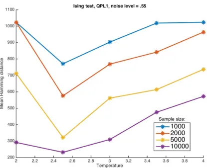
The general effects of varying temperature are highlighted in figure 4.2 using QPL1 with noise level 0.15. The results for all methods and noise levels follow roughly the same pattern: the best results are achieved with T=2.5 or T=3, while for both lower and higher temperatures the performance degrades. Increasing the sample size enhances the results.

(32)

Figure 4.2 – QPL1: Effects of changing temperature with different sample sizes. The effects are roughly similar for all methods and configurations tested.

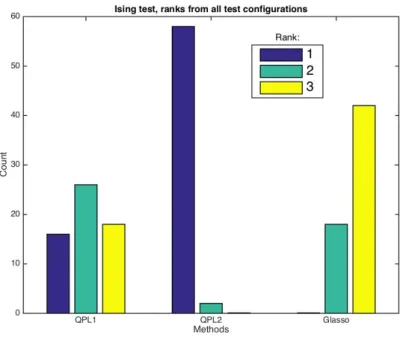
To assess the performance of each method compared to the other two, we calculate a ranking for each configuration of the test settings based on their average hamming distances. This leads to 60 rankings (5 temperatures * 3 noise levels * 4 sample sizes). In case of a tie, the tied methods are all awarded the best rank out of the tied ones (e.g. in a case where two methods have the same average hamming distance behind the best method, both of the tied methods get a rank of 2). The results are plotted in figure 4.3.

(33)

Figure 4.3 – QPLs & Glasso: Number of different rankings for each method in test 1. QPL2 clearly outperforms the other methods.

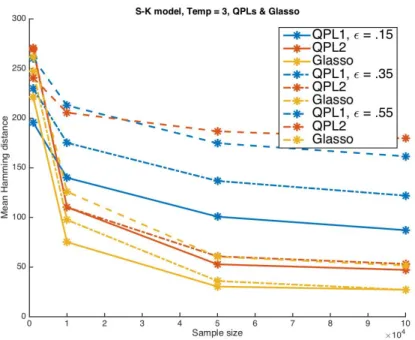
As can be seen from the results, in this test QPL1 tends to perform better than Glasso, and QPL2 is clearly superior to both other methods. The cases where QPL1 loses to Glasso correspond to the higher noise settings. As an example, figure 4.4 presents some of the results in the case ofT = 3.

(34)

Figure 4.4 – QPLs & Glasso: Temp=3. QPL1 tends to perform better than Glasso with low noise level (top). Glasso outperforms QPL1 with high noise level (bottom).

(35)

4.3.2 Second test: Sherrington-Kirkpatrick model

As a second testing setup, we use the S-K model. In this model, the interaction strengths are drawn randomly from a normal distribution, i.e. we set

Jj,i∼N(0,1/d), (4.7)

wheredis the number of variables. The result is that both the interaction strengths and the model topology are randomly generated.

This model presents some problems for the performance measurement, since interac-tions that are practically zero would still be counted as mistakes in learning. To avoid these kind of issues, we use a threshold of 0.15 for the interactions, i.e. all interactions with an absolute value smaller than the threshold value are set to zero.

This structure learning task is significantly harder than the one using regular Ising models. We increase the number of maximum observations to 105 and decrease the number of variables to 25, but otherwise the testing setup is kept unchanged.

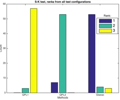
The ranks from all test configurations calculated as in the first test are plotted in figure 4.5. In this task, both QPL methods perform poorly compared to the Glasso, while QPL2 again outperforms QPL1 very systematically.

Figure 4.5 – QPLs & Glasso: Number of different rankings for each method in test 2. Glasso is clearly superior to the other methods.

Since the poor performance of QPLs persists with virtually all noise levels, it would seem that the problem is not mainly caused by the noise. To test this further, we also used MPL learning on the noiseless datasets withT = 2.5. As expected, the MPL results

(36)

are very similar to the QPL2 results with low noise settings (see figure 4.6). This lends some credence to the claim that the problem is related to the actual scoring used and not so much to the noise.

Figure 4.6 – QPLs & MPL with noise levels 0.15 (top) and 0.35 (bottom). QPL2 performance is very similar to MPL on lower noise levels.

(37)

4.3.3 Third test: Ising model with random interaction strengths

Based on the second experiment, the bad performance could be caused either by the interactions strengths, which are weak on average, or the more densely connected model topology; the average number of neighbours for a node is around 11. To further test these issues, as a third test setup we use the fixed 2D Ising model topology with 5∗5 = 25 nodes, but generate the interaction strengths randomly as in the S-K model. We also use a threshold = 0.15 in this setting, but since we do not want to randomize the topology, the interactions below the threshold are just randomly generated again until they are above the threshold level. We run the test with temperatureT = 3.

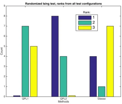
With this setting, both QPL methods perform better again (see ranks as in the previous tests in figure 4.7). QPL2 again performs consistently better than QPL1, while both QPLs outperform Glasso on lower noise settings and get left behind on high noise level (see figure 4.8 for examples). In the case of lower noise levels, the results therefore seem to point to the high number of neighbours as the primary reason for the bad performance on the S-K tests, although the high-noise & weak interactions combination is also a troublesome case.

Figure 4.7 – QPLs & Glasso: Number of different rankings for each method in test 3. QPL2 performs better than the other two methods.

(38)

Figure 4.8 – QPLs & Glasso: QPLs perform better on lower noise levels (top), while Glasso outperforms others on the highest noise level (bottom).

One logical remedy for the problems with denser graphs and weak interactions is to tweak the prior used, since the problem basically boils down to over-regularization; based on the previous tests, the equivalent sample size valueN = 1 used in the previous tests seems to correspond to quite a heavy penalty on denser connectivity between the

(39)

nodes. To set the prior in a more informed manner, we could resort e.g. to optimizing the prior strength on some separate training set similarly to the approach used with the Glasso parameter tuning.

4.3.4 Fourth test: Different priors on Ising model with randomized

interaction strengths

To see the effect of the prior on the results, we use the same datasets generated in the previous test with fixed 2D Ising topology and random interactions, but run the learning with different values for the equal sample size prior N. Examples of the results with

N ∈ {1,101,102,103,104,105} are plotted in figure 4.9. The results with other noise levels lead to the same conclusions. It seems that the prior can be used effectively to enhance performance in noisy environments with weak interactions. Based on this test, the prior strength should definitively be treated as a free parameter that needs to be set in an informed manner.

Figure 4.9 – QPL1 with varying prior strength and Glasso. Optimizing the prior value is clearly beneficial.

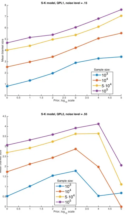
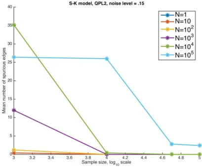
4.3.5 Fifth test: Different priors on Sherrington-Kirkpatrick model

As a final test, to gauge the effect of the prior with dense graphs and weak interactions, we use the same S-K model data generated in the second test with T = 3 with prior values N ∈ {1,101,102,103,104,105}. Similarly to the previous test, the prior strength can be tuned to improve the performance of both methods significantly. As already