w o r k i n g
p
a
p
e
r
F E D E R A L R E S E R V E B A N K O F C L E V E L A N D
10
02
Measuring Systemic Risk
by Viral V. Acharya, Lasse H. Pedersen, Thomas Philippon, and Matthew Richardson
Working papers
of the Federal Reserve Bank of Cleveland are preliminary materials circulated to stimulate discussion and critical comment on research in progress. They may not have been subject to the formal editorial review accorded offi cial Federal Reserve Bank of Cleveland publications. The views stated herein are those of the authors and are not necessarily those of the Federal Reserve Bank of Cleveland or of the Board of Governors of the Federal Reserve System.Working papers are now available electronically through the Cleveland Fed’s site on the World Wide Web:
Working Paper 10-02
March 2010
Measuring Systemic Risk
by Viral V. Acharya, Lasse H. Pedersen, Thomas Philippon, and Matthew Richardson
We present a simple model of systemic risk and show how each fi nancial insti-tution’s contribution to systemic risk can be measured and priced. An institu-tion’s contribution, denoted systemic expected shortfall (SES), is its propensity to be undercapitalized when the system as a whole is undercapitalized, which increases in its leverage, volatility, correlation, and tail-dependence. Institutions internalize their externality if they are “taxed” based on their SES. Through sev-eral examples, we demonstrate empirically the ability of components of SES to predict emerging systemic risk during the nancial crisis of 2007-2009.
Key words: systemic risk, risk pricing, systemic expected shortfall, risk internal-ization
JEL codes: G01, G18
The authors would like to thank Rob Engle for many useful discussions. They are grateful to Christian Brownlees, Farhang Farazmand and Hanh Le for excel-lent research assistance. The authors also received useful comments from seminar participants at Bank of England, Banque de France, International Monetary Fund, World Bank, Helsinki School of Economics, Bank for International Settlements (BIS), London School of Economics, Federal Reserve Bank of Cleveland, Federal Reserve Bank of New York, NYU-Stern, NYU-Courant Institute, Bank of Canada, MIT and NBER Conference on Quantifying Systemic Risk (especially Dale Gray and Matthias Drehman, discussants).
All the authors are at New York University, Stern School of Business, 44 West 4th St., New York, NY 10012. They can be reached at [email protected];
Failures of financial institutions can impose an externality on the rest of the economy, and the recent crisis provides ample evidence of the importance of containing this risk. However, current financial regulations, such as Basel I and Basel II, are designed to limit each institution’s risk (for example, market and credit value-at-risk) seen in isolation; they are not sufficiently focused on systemic risk. This is in spite of the fact that systemic risk is often the rationale provided for such regulation. As a result, while individual risks are properly dealt with in normal times, the system itself remains, or in some cases is induced to be, fragile and vulnerable to large macroeconomic shocks.1
Our goal in this paper is to propose a simple, alternative measure that focuses on systemic risk. To this end, we first develop a framework for formalizing and then measuring systemic risk. Second, given this framework, we formulate an optimal policy for managing systemic risk. Finally, we provide a detailed empirical analysis of the financial crisis of 2007-2009, giving support to our theoretical analysis of systemic risk.
It is important to recognize that value-at-risk (VaR), the dominant form of risk measure-ment in the financial sector, was invented by banks as an internal risk managemeasure-ment tool. VaR was meant to be useful for comparing risk across desks and asset classes within a bank. VaR was never meant to be a tool for regulating banks. The need for economic foundations for a systemic risk measure is more than an academic concern. We believe that lack of such a measure is at the root of practical failures of regulation.
It is of course difficult, if not impossible, to find a systemic risk measure that is at the same time practically relevant and completely justified by a general equilibrium model. The reason is that financial regulation can only be analyzed in economies with incomplete markets, moral hazard and information asymmetries. The problem, however, is that to date the gap between the theoretical recommendations and the practical needs of regulators has been so wide that measures such as institution-level VaR have persisted in assessing risks of the financial system as a whole.
1See Crockett (2000) and Acharya (2001) for an early recognition of this inherent tension between
Our strategy is to study a simplified theoretical model that is based on the common denominator of various models. We argue that two ideas are widely shared by economists and regulators. The first idea is that the main reason for regulating financial institutions is that there are externalities from their failures (or even just under-capitalization) that spill over to the rest of the economy. The second idea is that if these externalities are not internalized by financial institutions, then they manifest as excessive risk, leverage and herding in business and trading decisions of financial firms.
Given these two basic ideas, the critical step is to model the externalities. This is where we depart from the fully micro-founded models and instead use the stress tests of the spring of 2009 as a guide to learn about the type of externality that regulators and market participants seem to view as a first-order concern. Specifically, we assume that the externality depends on the aggregate capital shortfall in the financial industry.2 We then study the effect of
externality on risk choices of banks that maximize shareholder value given limited liability. The interesting point is that even such a simple model is enough to obtain a new and interesting theory of systemic risk regulation.3
A detailed description of the theoretical and empirical results follows.
Theoretical results: Our theory considers a number of financial institutions (“banks”) that must decide on how much capital to raise and which risk profile to choose in order to maximize their risk-adjusted return. A regulator considers the aggregate outcome of banks’ actions, additionally taking into account each banks losses during an idiosyncratic bank failure and the externality arising in a systemic crisis, that is, when the aggregate capital 2This assumption is consistent with models that spell out the exact nature of the externality, such as
models of (i) financial contagion through interconnectedness (e.g., Rochet and Tirole, 1996); (ii) pecuniary externalities through fire sales (e.g., several contributions compiled in Allen and Gale, 2007, and Acharya and Yorulmazer, 2007), margin requirements (e.g., Garleanu and Pedersen, 2007), liquidity spirals (e.g., Brunneremeier and Pedersen, 2009), and interest rates (e.g., Diamond and Rajan, 2005 and Acharya, 2009); and, (iii) runs (e.g., Diamond and Dybvig, 1983, and Pedersen, 2009).
3Our modeling finds natural parallels in the early work of Stigler (1971) and Peltzman (1976) on the
in the banking sector is sufficiently low.4 The pure market-based outcome differs from the regulator’s preferred allocations since, due to limited liability, banks do not take into account the loss they impose in default on creditors and the externality they impose on the society at large in a systemic crisis.
We show that to align incentives, the regulator optimally imposes a tax on each bank which is related to the sum of its expected default losses and its expected contribution to a systemic crisis, denoted Systemic Expected Shortfall (SES). Importantly, this means that banks have an incentive to reduce their tax (or insurance) payments and thus take into account the externalities arising from their risks and default. Additionally, it means that they pay in advance for any support given to the financial system ex post during a systemic crisis.
We show that SES, the systemic-risk component, is equal to the expected systemic costs when the financial sector becomes undercapitalized times the financial institution’s percent-age contribution to this under-capitalization. SES is therefore measurable and we provide theoretical justification for it being related to a financial firms marginal expected shortfall,
MES (i.e., its losses in the tail of the aggregate sector’s loss distribution), and to its leverage.
Empirical results: We empirically investigate three examples of emerging systemic risk in the financial crisis (focusing on large financial institutions based in the United States) and analyze the ability of our theoretically motivated measures to capture this risk. Specifically, we look at the relation between our measures and (i) capital shortfalls at large financial institutions estimated via stress tests performed by bank regulators during the Spring of 2009, (ii) realized systemic risk that emerged in the equity of large financial firms from July 2007 through the end of 2008, and (ii) realized systemic risk that emerged in the credit default swaps (cds) of large financial firms from July 2007 through the end of 2008.
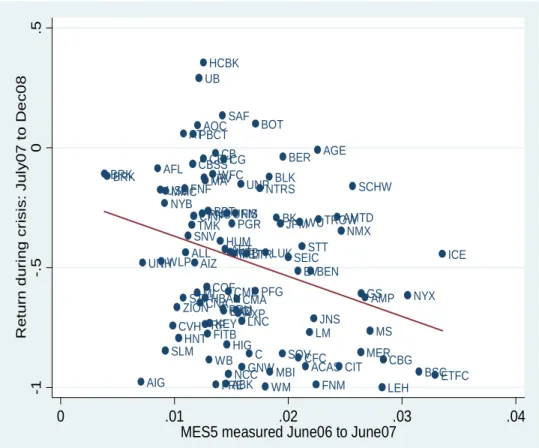
Figures 1, 2 and 5 provide a simple illustration of the ability of the firm’sMES to forecast realized systemic risk. In particular, the figures graph a cross-sectional scatter plot of the 4In the spirit of deposit insurance, we assume that part of the bank’s liabilities are insured, but our results
largest financial firm’s capital shortfalls (from the stress test exercise), realized equity returns and realized cds returns during the financial crisis respectively on each firm’s MES prior to the crisis. Each figure shows a clear relation between MES and systemic risk. Formal statistical analysis shows that the slope is statistically significant, and along with leverage,
MES loads significantly on the financial firms that ran aground during the crisis.
To mention one of the examples, we estimate our systemic risk measures for 102 financial firms in the US financial sector with equity market capitalization as of end of June 2007 in excess of 5bln USD (see Appendix B). We calculate the MES of each firm using the worst 5% days of the value-weighted market return from CRSP during the period June 2006 to June 2007, and leverage measured as of end of June 2007. To consider our measure’s ability to estimate each financial institution’s systemic risk taking, we check how well these risk measures calculated before the sub-prime crisis help predict which institutions fared the worst during the crisis period of July 2007 till December 2008. We find that both components of systemic risk MES and leverage contribute to explaining a significant proportion of the realized returns during the crisis (R2 of 27.34%). Importantly, standard measures of institution-level risk such as expected loss in institution’s own left tail and volatility do a relatively poor job, and the standard measure of covariance, beta, has a modest explanatory power.
To summarize, our theoretical analysis provides a conceptual framework for measuring a financial institution’s contribution to systemic risk, specifically as the losses it incurs when the system as a whole is under-capitalized. Our empirical analysis shows that such a cross-sectional measure of systemic risk can be estimated using market (equity and cds) data. Importantly, the measure is able to predict realized systemic risk contributions of financial firms during the crisis of 2007-2009. These results have important consequences for design of future regulation. One, they suggest that systemic risk measures such as ours may be valuable aids to regulators when they “stress test” balance-sheets of individual institutions to adverse macroeconomic and financial conditions. Second, they imply that the extent to which a firm is subject to macro-prudential regulation (say a tax, a capital requirement, or
forced debt-for-equity conversion) can be tied to its market-based measures of systemic risk. The remainder of the paper is organized as follows. Section 1 presents a quick review of firm level risk management. Section 2 lays out a model to define, measure and manage systemic risk. Section 3 discusses measurement issues associated with our systemic risk analysis. Of particular interest, motivation is given for two variables in particular, namely the firm’s
MES and leverage. Section 4 empirically analyzes the implications of our model for systemic risk during the financial crisis of 2007-2009. Section 5 relates our systemic risk measure to existing literature and methodologies. Section 6 concludes.
1
A Review of Firm Risk Management
In this section we review the standard risk measures used inside financial firms.5 This review allows us to define some simple concepts and intuitions that will be useful in our model of systemic risk. Two standard measures of firm level risk are Value-at-Risk (VaR) and Expected-Shortfall (ES). These seek to measure the potential loss incurred by the firm as a whole in an extreme event. Specifically, VaR is the most that the bank loses with confidence 1-α, where α is typically taken to be 1% or 5%. For instance, with α = 5%, VaR is the most that the bank loses with 95% confidence. Hence, VaR = −qα , where qα is the
α quantile of the banks return R:
qα =sup{z|P r[R < r]≤α} (1)
The expected shortfall (ES) is the expected loss conditional on something bad happening, that is, the loss conditional on the return being less than the a quantile:
ESα =−E[R|R ≤qα] (2)
Said differently, the expected shortfall is the average returns on days when the portfolio exceeds its VaR limit. We focus on ES because it is coherent and more robust than VaR.6
5See Yamai and Yoshiba (2005) for a fuller discussion.
6VaR can be gamed in the sense that asymmetric, yet very risky, bets may not produce a large VaR. The
For risk management, transfer pricing, and strategic capital allocation, banks need to break down firm-wide losses into contributions from individual groups or trading desks. To see how, let us decompose the bank’s return R into the sum of each group’s return ri, that is, R=P
iyiri, where yi is the weight of group i in the total portfolio. From the definition of ES, we see that:
ESα =− X
i
yiE[ri|R≤qα]. (3)
From this expression we see the sensitivity of overall risk to exposure yi to each group i:
∂ESα
∂yi
=−E[ri|R ≤qα]≡M ESαi, (4)
where M ESi is group i’smarginal expected shortfall. The marginal expected shortfall mea-sures how group i’s risk taking adds to the bank’s overall risk. In words, MES can be measured by estimating group i’s losses when the firm as a whole is doing poorly.
These standard risk-management practices can be useful for thinking about systemic risk. A financial system is constituted by a number of banks, just like a bank is constituted by a number of groups. We can therefore consider the expected shortfall of the overall banking system by letting R be the return of the aggregate banking sector. Then each bank’s contribution to this risk can be measured by itsMES. We now present a model where we model explicitly the nature of systemic externalities.
Indeed, one of the concerns in the ongoing crisis has been the failure of VaR to pick up potential “tail” losses in the AAA-tranches. ES does not suffer from this since it measures all the losses beyond the threshold. This distinction is especially important when considering moral hazard of banks, because the large losses because the VaR threshold are often born by the government bailout. In addition, VaR is not a coherent measure of risk because the VaR of the sum of two portfolios can be higher than the sum of their individual VaRs, which cannot happen with ES (Artzner et al., 1999).
2
Measuring Systemic Risk in an Economic Model
2.1
Banks’ Incentives
The economy hasN financial firms, which we denote as banks for short, indexed byi= 1, ..N
and two time periods t = 0,1. Each bank i chooses how much xi
s to invest in each of the available assets s= 1, ..S, acquiring total assets ai of
ai = S X
s=1
xis. (5)
These investments can be financed with debt or equity. In particular, the owner of any bank
i has an initial endowment ¯wi
0 of whichwi0 is kept in the bank as equity capital and the rest
is consumed or used for other activities. The bank can also raise debtbi. Naturally the sum of the assets ai must equal the sum of the liabilities, equity wi
0 and the debt bi, giving the
budget constraint:
w0i +bi =ai. (6)
At time 1, assets pays off ri
s per dollar invested for banki (so the net return is ris−1). We allow asset returns to be bank-specific to capture differences in investment opportunities. The total income of the bank at time 1 isyi = ˆyi−φi whereφi captures the costs of financial distress and the pre-distress income is
ˆ yi = S X s=1 rsixis. (7)
The costs of financial distress depend on the income and on the face value fi of the out-standing debt
φi = Φ ˆyi, fi
. (8)
Our formulation of distress costs is quite general. Distress costs can occur even if the firm does not actually default. This specification captures debt overhang problems as well as traditional costs of financial distress. We restrict the specification to φ ≤yˆso thaty≥0.
To capture various types of government guarantees, we assume that a fraction αi of the debt is implicitly or explicitly guaranteed by the government. The face value of the debt is set so that the debt holders break even, that is,
bi =αifi+ 1−αiEmin fi, yi. (9)
Although our focus is on systemic risk, we include government debt guarantees because they are economically important and because we want to highlight the different regulatory implications of deposit insurance and systemic risk. The insured debt can be interpreted as deposits, but it can also cover implicit guarantees. Technically, the pricing equation (9) treats the debt as homogeneous ex-ante with a fraction being guaranteed ex-post. This is only for simplicity and all of our results go through if we make the distinction between guaranteed and non-guaranteed debt ex-ante. (In that case, the guaranteed debt that the bank can issue would be priced at face value, while the remaining debt would be priced as above with α= 0.)
The net worth of the bank wi
1 at time 1 is
w1i = ˆyi−φi−fi (10)
The owner of the bank equity is protected by limited liability so it receives (1−Ii)w1i, where
Ii is the indicator of default by bank i:
Ii ≡1[wi
1<0]. (11)
The owner of the bank solves the following program: max wi 0,bi,{xis}s c· w¯i0−w0i −τi+Eu (1−Ii)·w1i , (12)
subject to (6)–(10). Here, ui(.) is the bank owner’s utility of time-1 income, ¯wi
0−w0i −τi
is the part of the initial endowment ¯wi
0 that is consumed immediately (or used for outside
activities). The remaining endowment is kept as equity capital wi
0 and or used to pay the
The parameterchas several interpretations. I can simply be seen as a measure the utility of immediate consumption, but, more broadly, it is the opportunity cost of equity capital. We can think of the owner as raising capital at cost c, we can think of debt as providing advantages in terms of taxes or incentives to work hard. What really matters for us is that there is an opportunity cost of using capital instead of debt.
2.2
Welfare, Externalities, and the Planer’s Problem
The regulator want to maximize the following welfare function: N X i=1 c· w¯0i −wi0−τi+E " N X i=1 ui (1−Ii)·w1i +g N X i=1 Iiαiwi1+e·I¯· z N X i=1 ai− N X i=1 w1i !# (13) This welfare function has three parts. The first part is the sum of the utilities of all the bank owners. The second part is the cost of the debt insurance program. The parameter
g captures administrative costs and costs of tax collection. The cost is paid conditional on default by firmi and a fraction αi of the shortfall is covered.
The third part of the welfare function captures the externality of financial crisis and is the main focus of our analysis. The parameter e measures the severity of the externality imposed on the economy when the financial sector is in distress. We define the indicator for the occurrence of systemic distress as capturing an event where the capital in the financial system falls below a fraction z of the aggregate assets:
¯
I = 1[PN i=1w1i<z
PN
i=1ai]. (14)
The critical feature that we want to capture is that of an aggregate threshold for capital needed to avoid early fire sales and restricted credit supply. Our specific formulation is the simplest one that captures this effect. The cost is zero as long as aggregate financial capital is above this threshold and grows linearly when it falls below. The externality depends only on the aggregate shortfall of capital in the financial sector. This is consistent with the emphasis of the stress tests performed by the US government in the spring odf 2009, and it is
the crucial difference between systemic and idiosyncratic risk. It means that a bank failure occurring in a well capitalized system imposes no externality to the economy. We believe this captures well the example of Barings Bank, for instance, whose failure in 1995 did not disrupt the global financial system. The Dutch bank ING purchased Barings and assumed all of its liabilities with minimal government involvement and no commitment of tax payer money. This stands in sharp contrast with the failures of Bear Stearns or Lehman Brothers. The planer’s problem is to choose a tax system that maximizes the welfare function (13) subject to the same technological constraints as the private agents. This ex-ante (time 0) regulation is relevant for the systemic risk debate, and this is the one we focus on. We do not allow the planner to redistribute money among the banks at time 1 because we want to focus on how to align ex ante incentives and because there are clear operational and informational constraints that prevent the government from quickly adjusting the marginal utilities in real time.7 In doing so, we follow the constrained efficiency analysis performed in the liquidity provision literature. In this literature, the planner is typically restricted to affect only the holding of liquid assets in the initial period (see Lorenzoni, 2008, for instance).
Lastly, we need to account for the taxes that the regulator collects at time 0 and the various costs borne at time 1. Since we focus on the financial sector and do not model the rest of the economy, we simply impose that the aggregate taxes paid by banks at time 0 add up to a constant:
X
i
τi = ¯τ . (15)
There are several interpretations for this equation. One is that the government charges ex-ante for the expected cost of the debt insurance program. We can also add the expected cost of the externality. At time 1, the government would simply balance its budget in each state of the world with lump-sum taxes on the non financial sector. We can also think of equation (15) as part of a larger maximization program, where a planner would maximize utility of banks owners and other agents. This complete program would pin down ¯τ, and we 7There would be three reasons for the planner to redistribute money ex-post: differences in utility
could then think of our program as solving the problem of a financial regulator for any given level of transfer between the banks and the rest of the economy.
2.3
Optimal taxation
Our optimal taxation policy has close parallels to the notion of “marginal expected shortfall” (MES) used to manage risk inside banks as explained carefully in Section 1. In acknowledg-ment of this connection, we define the default expected shortfall (DES) as the expected loss in bankruptcy for firm i:
DESi ≡ −EIi ·w1i
(16) Further, we define bank i’s systemic expected shortfall (SES) as its the amount its equity
wi1 drops below its target level, which is a fraction z of assets ai in case of a systemic crisis:
SESi ≡EI¯·(zai−w1i) (17)
The SES is the key measure of each bank’s expected contribution to a systemic crisis. Using these two functions we can characterize a tax system that would implement the optimal allocation. The regulator’s problem is to choose the tax schemeτ such as to mitigate systemic risk and inefficient effects of debt guarantees. The timing of the implementation is that the banks choose their leverage and asset allocations and then pay the taxes. The taxes are therefore conditional on choices made by the banks.
Proposition 1 The efficient outcome is obtained by a tax
τi = α ig c ·DES i+e c·SES i+τ 0, (18)
where τ0 is a lump sum transfer to satisfy equation (15).
Proof. Using the definition of τi in equation (18), the bank’s problem is max wi 0,bi,{xis}s c· w¯i0−w0i −τ0 +Eu (1−Ii)·w1i −αig·DESi−e·SESi,
and using (16) and (17), this becomes max wi 0,bi,{xis}s c· w¯i0−w0i −τ0 +Eu (1−Ii)·w1i +eI¯(zai−w1i) +αigIiw1i .
The set of programs for i = 1, ..., N is equivalent to the planer’s program and the budget constraint can be adjusted ed with τ0.
This result is intuitive. Each bank must first be taxed based on its expected losses in default DES to the extent that those losses are insured by the government, while recall that αi is the fraction of insured debt. The tax should be lower if raising bank capital is expensive (c > 1) and higher the more costly is government funds (g); A natural case is simply to think of g/c = 1 so that this part of the tax is simply an actuarial-fair deposit-insurance tax.8 Hence, this term in equation (18) corrects the underpricing of credit risk caused by the debt insurance program. We can write it as
DESi = Pr (Ii)·E
−wi1 |Ii
. (19)
DES is therefore the probability of default times the shortfall of net worth given default. The relevant point is that it is a measure of a bank’s own risk, irrespective of its relation to the system. In practice, the calculation of the expected shortfall is similar to a standard Value-at-Risk calculation.
The second part of the tax in (18) depends on the bank’s contribution to systemic risk as captured by SES, scaled by the severity e of the externality and scaled down by the bank’s cost of capital c. This forces the private banks to internalize the externality from aggregate financial distress. We can write it as
SESi = Pr ¯I·E(zai−w1i)|I¯. (20)
SES is therefore the probability of an aggregate crisis times the conditional loss of firm i in such a crisis. The important point is that the expectation is conditional on a macroeconomic shortfall. This calculation is similar to that of marginal risk within financial firms. In 8Note that it is important for incentives to keep charging this tax even if the FDIC fund collected over
marginal risk calculation, the risk managers ask how much a particular line of business is expected to lose on days where the firms hits its VaR constraint. Our formula applies this idea to the economy as a whole.
The optimal tax system holds for all kinds of financial distress costs and the planner reduces its taxes when capital is costly at time 0 (c is high). The fact that we obtain an expected shortfall measure comes from the shape of the externality function. It is important to understand the information required to implement the systemic regulation. The planner does not need to know the utility functions and investment opportunity sets of the various banks. It needs to estimate two objects: the probability of an aggregate crisis, and the conditional loss of capital of a particular firm if a crisis occurs.
3
Measuring Systemic Risk
The optimal policy developed in Section 2 calls for a fee (i.e., a tax) equal to the sum of two components: (i) an institution-risk component, i.e., the expected loss on its guaranteed liabilities, and (ii) asystemic-risk component, namely, the expected systemic costs in a crisis (i.e., when the financial sector becomes undercapitalized) times the financial institution’s percentage contribution to this undercapitalization. Some comments are in order.
There is much discussion amongst regulators, policymakers and academics of the need for a resolution fund that would be used to bailout large, complex financial institutions. This fund would be paid for by the institutions themselves and is akin to the FDIC. This resolution fund is essentially the institution-risk component of the above tax and reflects the optimal policy that government guarantees in the system (e.g., deposit insurance and too-big-to-fail) need to be priced. It does not, however, address the systemic risk of the financial firms as there is no differentiation between different economic states. Specifically, there is the belief that costs associated with financial firm losses are significantly higher in a crisis.
part is broken up into the product of two terms. The first term expected systemic costs -measures the level of the tax. There is growing evidence on what leads to financial crises and the large bailout costs and real economy welfare losses associated with banking crises (see, for example, Caprio and Klingebiel (1996), Honohan and Klingebiel (2000), Hoggarth, Reis and Saporta (2002), Reinhart and Rogoff (2008), and Borio and Drehmann (2009)). The bottom line from these studies is that there are leading indicators for banking crises, and these crises represent significant portions of GDP, on the order of 10%-20%. The important point is that, depending on the likelihood of a crisis, the systemic-risk component of the tax may be quite important.
The second term – % contribution of the financial institution to losses incurred by a financial sector collapse - determines which institutions pay more tax. That is, the main object of interest for the regulation of systemic risk is the expected dollar loss of capital of a firm conditional on the occurrence of a crisis. In practice, to implement the optimal policy, the planner needs to estimate the conditional expected losses before a crisis occurs. Our theory says that the regulator should use any variable that can predict capital shortfall in a crisis. In order to improve our economic intuition and to impose discipline on our empirical analysis, it is important to have a theoretical understanding of the variables that are likely to be useful for these predictions.
3.1
Measuring Systemic Risk: Intuition
A large focus of regulators and policymakers on managing systemic risk has been on the size of financial institution’s assets and/or liabilities. The theory described in Section II gives some support for this approach. Almost trivially, ceteris paribus, the expected losses of a financial firm conditional on a crisis are tied one-for-one to the size of the firm’s assets. In fact, Appendix B of the paper provides the % contribution of each firm’s $ MES across the 102 largest financial firms (i.e., firms with over $5 billion of market equity). The top 6 in terms of contribution (Citigroup (4.87%), JP Morgan (3.60%), Bank of America (3.54%), Morgan Stanley (2.51%), Goldman Sachs (2.41%) and Merrill Lynch (2.25%)) are also in the
top 7 in terms of total number of assets. Of course, even though a firm that doubles its size would pay, to a first approximation, twice the systemic tax, the firm would also have twice the cash flow to cover the tax. Therefore, from an economic point of view, the interesting question is what variables help explain the % expected losses (as opposed to $ losses).
Our theory says that the regulation of systemic risk should be based on SES. Equation (20) shows that there are two main pieces to estimate. The first is the probability P r I¯
of a systemic event. The unconditional risk can be measured using historical research as in Reinhart and Rogoff (2008). The conditional risk can be inferred from dynamic long-run volatility models and implied volatilities for long-dated assets from option prices (Engle, 2009).
We focus on the cross-sectional part. Control for each bank’s size, we scale by initial equity wi
0, which gives the following cross-sectional variation in systemic riskSES:
SESi wi 0Pr ¯I = zai wi 0 −1−E wi 1 wi 0 −1|I¯ .
The first part, zawii
0 −1, measures whether the leverage
ai wi
0 is initially already “too high”.
Specifically, since systemic crises happen when aggregate bank capital falls below z times assets, z times leverage should be less than 1. Hence, a positive value of zawii
0 − 1 means
that the bank is already under-capitalized at time 0. We can think of z as being in the range of 8% top 12%. The second term is the expected equity return conditional on the occurrence of a crisis. Hence, the sum of these two terms determine whether the bank will be under-capitalized in a crisis.
In practice, the planner needs to estimate the conditional expected losses before a crisis occurs. Our theory says that the regulator should use any variable that can predict capital shortfall in a crisis. In order to improve our economic intuition and to impose discipline on our empirical analysis, it is important to have a theoretical understanding of the variables that are likely to be useful for these predictions so we want to relateSES to observed equity returns.
We can think of the ¯I events in our model as extreme tail events happening once a decade or less (in the US at least). In the meantime, we observe “normal” tail events. Let us define
these events as the worst 5% market outcomes at daily frequency which we denote by I5%.
Based on these events, we can define a marginal expected shortfall (MES) using net equity returns of firm iduring these bad markets outcomes
M ES5%i ≡ −E w1i wi 0 −1|I5% .
We measureMES using a sample of negative market returns, but typically without observing a default so we can think of equity value as being always positive in the sample ofI5% events.
We now state our assumption regarding the tail behavior of asset returns.9 We assume that returns follow
rsi =ηsi −δi,sis−βi,sm,
where ηi
s follows a thin-tailed (Gaussian for instance) distribution while is and m follow independent normalized power law distributions with tail exponent ζ. Power laws dominate in the tail so we have the following simple properties (Gabaix, 2009). First, the VaR of ri s at level q is V aR(ri
s;q) =
δi,sζ +βi,sζ 1/ζq−1/ζ, and the corresponding Expected Shortfall is ES(ri
s;q) = ζ
ζ−1V aR(r
i
s;q). Second, since the shock m is the source of systemic risk, the events I% and ¯I correspond to critical values %
m and ¯m respectively. Note that there is a direct link between the likelihood of an event and its tail size, since we have ¯m
%m =
Pr(I5%) Pr(I¯)
1/ζ
. Using the power laws, we obtain the following proposition.
Proposition 2 The systemic expected shortfall is related to the marginal expected shortfall according to SESi Pr ¯I wi 0 = za i wi 0 −1 +k×M ES5%i + ∆i (21) where k≡ ¯m %m and ∆i ≡ E[φi|I¯]−k·E[φi|I5%] wi 0 −(k−1)fiw−ibi 0 .
9 Note that if we assume returns are multivariate normal, then the drivers of the firm’s % systemic
risk would be entirely determined by the expected return and volatility of the aggregate sector return and volatility, and their correlation. However, there is growing consensus that the tails of return distributions are not described by multivariate normal processes and much more suited to that of extreme value theory (e.g., see Barro (2006), Backus, Chernov and Martin (2009), Gabaix (2009) and Kelly (2009)). Our discussion helps clarify what variables are needed to measure systemic risk in the presence of extreme values.
Proof. Equity returns are given by wi1 wi 0 −1 = PS s=1risxis−φi−fi wi
0 −1.This allows us to write
M ES5%i = S X s=1 xis wi 0 E−ris |I5% + E[φ i |I 5%] wi 0 + f i−bi wi 0
In expectations we haveE[−ris|I5%] =βi,sζ−ζ1 %
mand thereforeE
−ris |I¯=kE[−rsi |I5%].
Using the definition of SES we can write 1 + SES i w0Pr ¯I = zai wi 0 −E wi 1 wi 0 −1|I¯ = za i wi 0 + S X s=1 xi s w0 E −rsi |I¯ +E φi |I¯ w0 + f i−bi w0
Under the power law assumption 1 + SES i w0Pr ¯I −k·M ES i = za i wi 0 +E φi |I¯−k·E[φi |I5%] w0 + (1−k)f i−bi wi 0 .
We see that SES has three components: Excess ex ante leverage zawii
0 −1, the measured
marginal expected shortfall MES using pre-crisis data, scaled up by k to account for the worse performance in the true crisis, and ∆i which comes from two sources. The termfi−bi
measures the excess returns on bonds due to credit risk. This difference is fixed and does not scale up so by multiplying MES by k we would overestimate SES by k−1 times the fixed payments.
The term Eφi |I¯−k ·E[φi |I5%] measures the excess costs of financial distress. It
is potentially more significant because we do not expect these costs to scale up with k as returns do. In practice, our estimation sample contains bad market days, but no real crisis. In these “normal” bad days we do not expect to pick up significant costs of distress. In other words, we are likely to measure E[φi |I5%] ≈ 0. On the other hand, we definitely
expect E
φi |I¯
to be significant, especially for highly levered firms. We therefore expect
MES to underestimate SES for highly levered firms. In essence, our formula (21) assumes that the I5% events capture the power law that dominates tail risk. This is probably a
fair assumption in commercial and investment banking. On the other hand, there could be a more significant bias in industries such as insurance where the industry leaders were all rated AAA before the crisis and distress or tail risk can only be seen in the most extreme
events.10 Also in these cases, equity market data may be somewhat less suitable or adequate compared to cds market data: By construction, cds fee is (approximately) the price of a tail risk event, namely the firm’s default, and hence conveys more direct information about tail risk of the underlying firm than the firm’s equity price does. Our empirical analysis to follow will employ both equity and cds data.
4
Empirical Analysis of the Crisis of 2007-2009
The theory of systemic risk presented in Section 2 and the underlying measurement issues described in Section 3 suggest that the relative systemic risk across firms can be measured cross-sectionally by just a few variables, two in particular being the marginal expected short-fall MES and leverage of the firm.
With respect to the former, we empirically estimate MES at a standard risk level of
α=5% using daily data of equity returns from CRSP.11 This means that we take the 5%
worst days for the market returns (R) in any given year, and we then compute the average return on any given firm (Rb) for these days. Even though these days clearly do not capture the tails of a financial crisis, we motivate its use via our power law analysis in Section 3.1. With respect to leverage, as shown by the current financial crisis, it is not straightforward to measure true leverage due to limited market data and breakdown of off- and on-balance sheet financing. Nevertheless, we apply the usual approach to measuring leverage. Specifically, since market value of debt is generally unavailable, it is standard instead to use the quasi-market value of assets. This is computed as [book value of assets book value of equity 10Another way of saying this is that firms that are in the business of writing insurance against tail risks
are less amenable to measurement of systemic risk using their normal time market data. Examples of such insurance are selling of deep out-of-the-money put options on the market, credit default swaps on portfolios of loans and mortgages (as were sold by A.I.G.), or liquidity puts to conduits (as was the case with Citigroup, documented by Acharya, Schnabl and Suarez, 2009). Acharya, Cooley, Richardson and Walter (2010) propose that “manufacturing tail risk” in this manner might have become the evolving business model of banking during 2004-2007 precisely to game the regulatory structure centered on measuring individual bank risks.
+ market value of equity]. The book characteristics of firms are available at a quarterly frequency from CRSP-Compustat merged dataset. We call the ratio of quasi-market value of assets to market value of equity as LVG in the empirical analysis to follow. 12
In this section, we investigate three examples of emerging systemic risk in the financial crisis and analyze the ability of the theoretically motivated measures to capture this risk. Specifically, we look at the relation between our measures and (i) capital shortfalls at large financial institutions estimated via stress tests performed by bank regulators during the Spring of 2009, (ii) realized systemic risk that emerged in the equity of large financial firms from July 2007 through the end of 2008, and (ii) realized systemic risk that emerged in the credit default swaps (cds) of large financial firms from July 2007 through the end of 2008.
In brief summary, across all three examples, the results are consistent with implications of the theory. In particular, simple measures of systemic risk implied by the theory have useful information for which firms ran aground during the financial crisis.
4.1
The Supervisory Capital Assessment Program
At the peak of the financial crisis, in late February 2009, the government announced a series of stress tests were to be performed on the 19 largest banks over a two-month period. In particular, known as the Supervisory Capital Assessment Program (SCAP), the Federal Reserve’s goal was to provide a consistent assessment of the capital held by these banks. The question asked on each bank was how much of an additional capital buffer, if any, each bank would need to make sure it had sufficient capital if the economy got worse and the financial crisis started up again.
In early May of 2009, the results of the analysis were released to the public at large. A total of 10 banks were required to raise $74.6 billion in capital. The SCAP was generally considered to be a credible test with bank examiners imposing severe loss estimates on 12A sample calculation here would be useful. As presented in Appendix B, in June 2007, theMES of Bear
Stearns is 3.15% and itsLVG is 25.62. That is, its average loss on 5% worst case days of the market was 3.15% and its quasi-market assets to market equity ratio was 25.62.
residential mortgages and other consumer loans, not seen since the Great Depression. The SCAP is an especially useful period to analyze to gauge the systemic risk measures described in this paper. The SCAP can be considered as close as possible to an ex ante
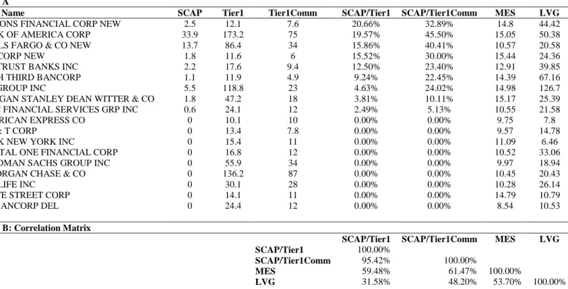
estimate of expected losses in a financial crisis. The regulators spent two months examining the portfolios and financing of the largest banks with a particular emphasis on creating consistent valuations across these banks. Table 1 provides a summary of each bank, including its shortfall (if any) from the SCAP at the end of April 2009, its tier 1 capital (so called core capital including common shares, preferred shares, and deferred tax assets), its tangible common equity (just its common shares), its measured MES (from April 2008 to March 2009) and its quasi market leverage. Five banks, as a percent of their Tier 1 capital, had considerable shortfalls, namely Regions Financial (20.66%), Bank of America (19.57%), Wells Fargo (15.86%), Keycorp (15.52%) and Suntrust Banks (12.50%).13
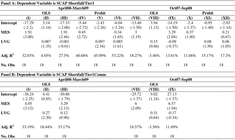
The question is how well do the systemic risk measures capture the SCAP estimates of systemic losses across these 17 firms? Table 2 provides an OLS regression analysis of both
MES and leverage on the SCAP shortfall as a percent of tier 1 capital (panel A) and tangible common equity (panel B). Because a number of firms have no shortfall, and thus there is a mass of observations at zero, we also extend the OLS regressions to a Probit analysis.
MES is strongly significant in both the OLS and Probit regressions. For example, in the OLS regressions of MES on tier 1 capital and tangible common equity respectively, the t-statistics are 3.00 and 3.12 with adjusted R-squareds of 32.03% and 33.19%. When leverage is added, the adjusted R-squareds either drop or are marginally larger. Not surprisingly, the adjusted R-squareds jump considerably for the Probit regressions, with the tier 1 capital regressions reaching 40.68% and, with leverage included, 53.22%. The important point is 13The interested reader might be surprised to see that, although it required additional capital, Citigroup
was not one of the leading firms. It should be pointed out, however, that towards the end of 2008 Citigroup received $301 billion of federal asset guarantees on their portfolio of troubled assets. Conversations with the Federal Reserve confirm that these guarantees were treated as such for application of the stress test. JP Morgan and Bank of America also received guarantees (albeit in smaller amounts) through their purchase of Bear Stearns and Merrill Lynch, respectively.
that the systemic risk measures seem to capture quite well the SCAP estimates of % expected losses in a crisis.
As an additional analysis, the same regressions were run using MES and leverage mea-sured prior to the failure of Lehman Brothers in mid September 2008, in other words, us-ing information from October 2007 to September 2008. While the results are in general agreement with the earlier ones, in particular MES is statistically significant, the adjusted R-squareds drop considerably for both measures of capital and for both the OLS and Probit Regressions with a range of 11% to 18%. Of course, the Federal Reserves SCAP would also have been considerably different prior to Lehman Brothers failure.
4.2
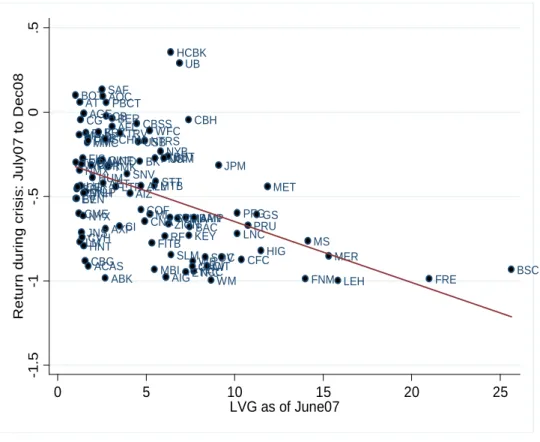
The Financial Crisis: July 2007 to December 2008
To illustrate the computation of our systemic risk measures and their power in explaining the performance of firms during a systemic crisis, we focus on a “demo” period surrounding the subprime crisis. We consider 102 financial firms in the US financial sector with equity market capitalization as of end of June 2007 in excess of 5bln USD. Appendix A lists these firms and their “type” based on two-digit SIC code classification (Depository Institutions, Securities Dealers and Commodity Brokers, Insurance, and Others). For sake of illustration, we use the CRSP value-weighted index as the “market”. Note that our model suggests the market should be the aggregate of the firms under investigation and we examine robustness of our results to financial sector aggregate as the market. We use daily stock return data from CRSP.
The overall idea is to estimate the ex ante MES and leverage using data from the year prior to the crisis (June 2006 till June 2007) and use it to explain the cross-sectional variation in performance during the crisis (July 2007 till December 2008). As explained in Section 3.1, we identified two inputs: first, the Marginal Expected Shortfall MES, which we choose to compute at 5% worst case days for the market, and second, the leverage of each firm l.
While analyzing the performance of MES and LVG, it is important to also check their incremental power relative to other measures of risk. For this, we focus on measures of
firm-level risk: the expected shortfall, ES (i.e., the negative of the firm’s average stock return in its own 5% left tail), and the annualized standard deviation of returns based on daily stock returns, Vol. We also look at the standard measure of systematic risk, Beta, which is the covariance of a firm’s stock returns with the market divided by variance of market returns. Thus, the difference between oursystemicrisk measureBeta arises from two sources: systemic risk is based on tail dependence rather than average covariance, and it is corrected for leverage of the firm. We want to compare these ex ante risk measures to the ex post
Event Return, that is, the realized return of financial firms during the period July 2007-Dec 2008.
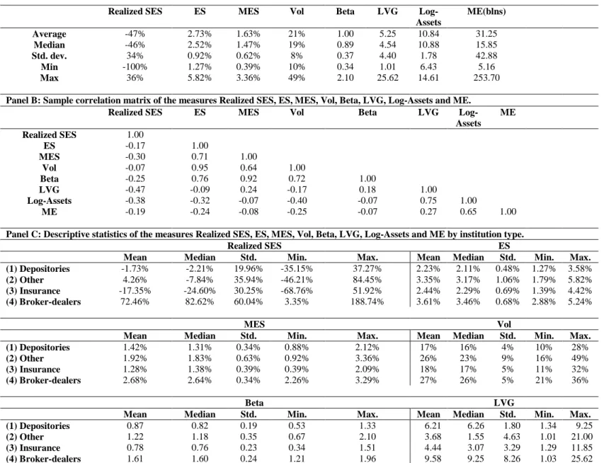
Table 3 describes the summary statistics of all these risk measures, where Panel A re-ports the univariate statistics and Panel B the pair-wise correlations. The Event Return in Panel A illustrate how stressful this period were for the financial firms, with mean (median) return being−46% (−47%) and several firms losing their entire equity market capitalization (Washington Mutual, Fannie Mae and Lehman Brothers). It is useful to compare ES and
MES. While the average return of a financial in its own left tail is −2.73%, it is −1.63% when the market is in its left tail. The market itself has anES of −1.4% implying that the equally-weighted average return of financials when market is in its left tail is worse than the value-weighted average return (which is of course the market itself). Average volatility of financial stock returns are 21% with a beta of 1.0. The power law application in Section 3.1 suggests that an important component of systemic risk is LVG, the quasi-market assets to market equity ratio. This measure is on average 5.26 (median of 4.59), but it has several important outliers. The highest value of LVG is 25.62 (for Bear Stearns) and the lowest is just 1.01. All these measures however exhibit substantial cross-sectional variability, which we attempt to explain later.
Panel B shows that individual firm risk measures (ES andVol) are highly correlated, and so are dependence measures between firms and the market (MES andBeta). Naturally, the realized returns during the crisis (realized SES) are negatively correlated to the risk measures and, interestingly, realized SES is most correlated with LVG, Log-Assets and MES, in that
order.
We also examine the behavior of risk and systemic risk across types of institutions based on the nature of their business and capital structure. As shown in Appendix A, we rely on four categories of institutions: (1) Depository institutions (29 companies with 2-digit SIC code of 60); (2) Miscellaneous non-depository institutions including real estate firms whom we often refer to as “Other” (27 companies with codes of 61, 62 except 6211, 65 or 67); (3) Insurance companies (36 companies with code of 63 or 64); and (4) Security and Commodity Brokers (10 companies with 4-digit SIC code of 6211. 14
Panel C provides the univariate statistics of all the relevant risk measures by institution type. There are several interesting observations to be made. Depository institutions and insurance firms have lower absolute levels of risk, measured both by ES and Vol. These institutions also have lower dependence with the market,MES andBeta. The leverage, quasi-market assets to equity ratio, is however higher for depository institutions and securities dealers and brokers. When all this is in theory combined into our estimate of systemic risk measure, in terms of realized SES, insurance firms are overall the least systemically risky, next were depository institutions, and most systemically risky are the securities dealers and brokers. Importantly, by any measure of risk, individual or systemic, securities dealers and brokers are always the riskiest. In other words, the systemic risk of these institutions is high not just because they are riskier in an absolute risk sense, but they have greater tail dependence with the market (MES) as well as the highest leverage (LVG); in particular, their MES is about twice the median MES of financial firms and their leverage is twice as high as the median leverage of financial firms.
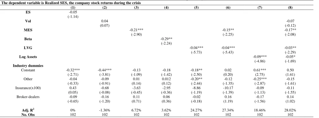
Table 4 and Figures 2 and 3 show the power ofMES and leverage in explaining the realized performance of financial firms during a systemic crisis. In particular, Table 2 contains cross-sectional regressions of realized returns during July 2007-Dec 2008 on the pre-crisis measures 14Note that Goldman Sachs has a SIC code of 6282 but we classify it as part of the Security and Commodity
Brokers group. Some of the critical members of other category are American Express, Black Rock, various exchanges, and Fannie and Freddie, the latter being of course significant candidates for systemically risky institutions.
of risk, MES, LVG, Log Assets, Vol, Beta and ES, respectively, and Figures 2 and 3 show the corresponding scatter plots. (We also note that Appendix B provides the firm-level data onMES and LVG.)
Figure 2 shows that MES does a reasonably good job of explaining the realized returns (R2 of 6.72%), and naturally a higherMES is associated with a more negative return during the crisis. A few cases illustrate the point well. We can see that Bear Stearns, Lehman Brothers, CIT and Merrill Lynch have relatively high MES and these firms lose a large chunk of their equity market capitalization. There are, however, also some reasons to be concerned. For example, exchanges (NYX, ICE, ETFC) have relatively highMES but we do not think of these as systemic primarily because they are not as leveraged as say investment banks are.
Similarly, while A.I.G. and Berkshire Hathaway have relatively lowMES, A.I.G.’s leverage at 6.12 is above the mean leverage whereas that of Berkshire is much lower at 2.29 and thus the two should be viewed differently from a systemic risk standpoint. Figure 3 shows that leverage does even better at explaining the realized returns (R2 of 24.27%), and the combination of MES and LVG show an even better fit:
Realized return= 0.02−0.12[1other]−0.01[1Insurance]
+ 0.16[1broker−dealer]−0.15M ES∗−0.04LV G∗ (22)
with anR2=27.34%. Thus adjustingMES for leverage of financial firms helps understanding
their systemic risk better.
In this light, exchanges are no longer as systemic as investment banks and A.I.G. looks far more systemic than Berkshire Hathaway. Further inspection of the firm-level data (Appendix B) reveals that the five investment banks rank in top ten both by their MES and leverage rankings, but this stability across measures is not a property of all other firms. For example, Countrywide is ranked 24th byMES given itsMES of 2.09%, but given its high leverage of 10.39 has a combined ranking of 6th using equation 22 (labeled in Appendix B as “Fitted Rank”). Similarly, Freddie Mac is ranked 61st by its MES but given its high leverage of 21 (comparable to that of investment banks), it ranks 2nd, in terms of its combined ranking. On
the flip side, CB Richard Ellis, a real-estate firm, has 5th rank inMES but given low leverage of 1.55 ranks only 24th in terms of combined ranking. Investment banks, Countrywide and Freddie all collapsed or nearly collapsed, whereas CB Richard Ellis survived, highlighting the importance of the leverage correction in systemic risk measurement.
In contrast to the statistically significant role ofMES in explaining cross-sectional returns, traditional risk measures Beta and ES do not perform that well. The R2 with Beta is just
3.62% and that withES is basically 0.0%. These results are also summarized in Table 4 which has three additional results. First, column (3) shows thatVol, another measure of individual firm risk does very poorly in explaining realized returns, in fact with essentially zero R2. Second, in the regressions that includeLVG and MES together, institutional characteristics no longer show up as significant. This suggests that the systemic risk measures do a fairly good job of capturing, for example, the risk of broker dealers. Third, column (8), however, shows that the log of assets comes in quite strong with an R2 around 18.5%. While its significance drops substantially once leverage is included, it still shows up in the regression analysis. The negative sign on log of assets suggests that size not only affects the $ systemic risk contribution of financial firms but also the % systemic risk contribution as well. In particular, large firms create more systemic risk than a likewise combination of smaller firms.
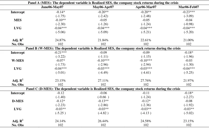
Figure 4 graphs a scatter plot of the MES computed during June 2006-June 2007 versus that computed during June 2005-2006. Even though there is no overlap between the return series, the plot generally shows a fair amount of stability from year to year with this particular systemic risk measure. Wide time-series variation in relative MES would make the optimal policy more difficult to implement. It is of interest therefore to examine how earlyMES and
LVG predict the cross-section of realized returns during the crisis. We compute MES and
SES over several periods other than the June 2006-07 “demo” period: June 06-May 07, May 06-Apr 07, Apr 06-Mar 07 and Mar 06-Feb 07. In each period, we use the entire data of daily stock returns on financial firms and the market, and the last available data on book assets and equity to calculate quasi-market measure of assets to equity ratio. Once the measures
are calculated for each of these periods, the exercise is always to explain the realized returns during the same crisis period of July 2007 to December 2008.
In contrast with Figure 4, Panel A shows that the predictive power ofMES progressively declines as we use lagged data for computing the measure. The overall predictive power, however, remains high as leverage has certain persistent, cross-sectional characteristics across financial firms. The coefficients on LVG remain unchanged throughout these periods. To better understand theMES decline, we repeat the Panel A regressions using two alternative measures of MES: (i)W-MES, a weighted MES, which uses exponentially declining weights (λ= 0.94 following the Risk Metrics parameter) on past observations to estimate the average equity returns on the 5% worst days of the market, and (ii) D-MES, a dynamic approach to estimating MES, which uses a dynamic conditional correlation (DCC) model with fat idiosyncratic tails.15 Panel B and Panel C provide the results for W-MES and D-MES,
respectively. The adjusted R2s are generally higher and the alternative measures of MES
better hold their predictive power. For example, the coefficients are still strongly significant using the April06-Mar07 data, with the t-statistics and R2s equal to (−1.24, −2.94, −2.36) and (22.61%, 27.76%, 24.58%) respectively for MES, W-MES and D-MES. These results suggest there is some value to exploring more sophisticated methods for estimating MES.
4.3
Using CDS to Measure Systemic Risk
Section IV.B above illustrated the ability of the MES and leverage of financial firms to forecast the equity performance of the 102 largest financial firms during the financial crisis period of July 2007 to December 2008. In this subsection, we add to this evidence by focusing on the credit default swaps (cds) of these same financial firms. Of the 102 financial firms, 40 of them have enough unsecured long-term debt to warrant the existence of cds in the credit derivatives market. Appendix C provides a list of the 40 firms, their type of institution, and stylized facts about their MES based on the cds market, including ranking, MES%, and 15We are grateful to Christian Brownlees and Robert Engle of New York University Stern School of
realized CDS spread returns during the crisis period.
A few important issues arise using cds data. The first question arises how to operational-ize the cds data for calculating MES. The cds premium resembles the spread between risky and riskless floating rate debt, denote this spread as s. To garner some intuition, note that
dP/P = −Dds and dP/P = ξdV /V, where P is the bond price, V the value of the firm’s assets, ξ is the elasticity of the bond price to firm value, and D is the bond’s duration. Combining the two relationships, we obtain that ds = −ξ/DdV /V. Ignoring the duration term changes across firms/days means that measuring the firm’s losses, i.e.,dV /V, using the spread change ds is proportional to its bond elasticity ξ. Since we know that ξ is approxi-mately 0 when the bond is close to risk-free and approxiapproxi-mately 1 when the bond is virtually in default,dsattaches close to zero weight todV /V for safe firms (when leverage is very low) and high weight (equal to 1/D) to dV /V for very risky firms (when leverage is very high). Therefore, a better measure of firm value changes is ds/s =−ξ/(Ds)dV /V, where s is tiny when eta is close to zero ands is large when eta is close to one.
In terms of thecds MES, therefore, we empirically estimateMES at a standard risk level of 5% using daily data of cds returns,ds/s, from the data provider Bloomberg.16 This means
that we take the 5% worst days for an equally-weighted portfolio of cds returns on the 40 financial firms from June 2006 to July 2007, and we then compute the cds return for any given firm for these days.17 Appendix C provides some interesting stylized facts given the fact that the cds MES estimates are all pre-crisis. Consider the top 3 financial institutions in terms of highest cds MES in each institutional category:
• The 3 insurance companies are Genworth Financial (16.40%), Ambac Financial (8.05%) and MBIA (6.71%). All of these companies were heavily involved in providing financial guaranties for structured products in the credit derivatives area.
• The top 3 depository institutions are Wachovia (7.21%), Citigroup (6.80%) and Wash-16Our results are robust to the sample of firms for which data are available from Markit, and the overlapping
sample of firms between Bloomberg and Markit.
ington Mutual (6.15%). These institutions are generally considered to ex post have been most exposed to the nonprime mortgage area, with two of them, Wachovia and Washington Mutual, actually failing.
• The top three broker dealers are Merrill Lynch (6.3%), Lehman Brothers (5.44%) and Morgan Stanley (4.86%). Two of these three institutions effectively failed.18
• The top three others, SLM Corp (6.82%), CIT Group (6.80%) and Fannie Mae (5.70%), also ran into trouble due to their exposure to credit markets, with both CIT going bankrupt and Fannie Mae being put into conservatorship.
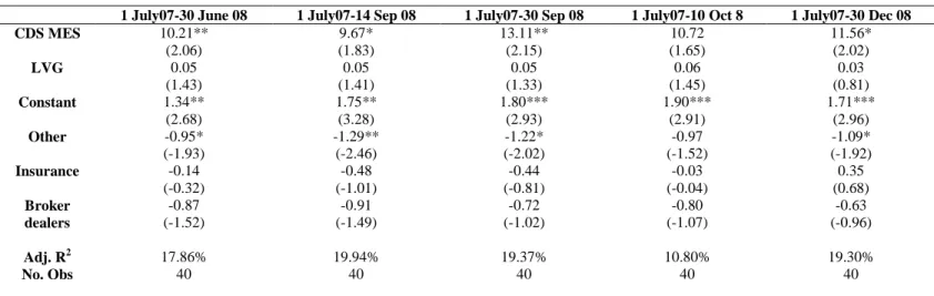
Even putting these results aside, the second issue is that cds may not reflect predicted losses of the financial firm to the extent some firms have more government guarantees as part of their capital structure, such as deposit institutions, the government sponsored enterprises and so-called too-big-to-fail firms.19 Since cds reflect estimated creditor losses, the backstop will lead to pricing distortions cross-sectionally. As a result, in terms of systemic risk, we analyze the ability ofcds MES to forecast systemic risk in both the July 2007 to December 2008, and the July 2007 to June 2008 period (i.e., prior to many government guarantees being made explicit). To further address this issue, we also investigate the ability of cds MES to forecast not only future CDS returns, but also equity returns.
Figures 5-8 respectively show scatter plots of cds MES on realized CDS returns in the July 2007-June 2008 and July 2007-December 2008 period, and on realized equity returns in the July 2007-June 2008 and July 2007-December 2008 period. The results are also strongly supportive of the ability of cds MES to forecast future changes in firm value during a financial crisis, whether estimated by cds or equity returns. To the point above, the 18We note here that if Bear Stearns cds return were measured until the point of its arranged merger with
J P Morgan in mid-March 2008, its realized cds return would be higher than having measured it till dates thereafter.
19Equity also suffers from this problem to the extent government guarantees delay bankruptcy and thus
extend the option of the firm to continue. It is more likely a second order effect, however, compared to the pricing of the underlying debt of financial firms in distress.
slope line is slightly flatter (steeper) for cds (equity) returns in the December 2008 end of sample period versus the June 2008 period. Since the crisis got considerably worse during the latter 6 months of 2008, this finding is consistent with the government making a number of guarantees explicit (e..g, the government sponsored enterprises, A.I.G., and in general the capital assistance programs related to TARP).
Table 6 provides summary statistics forcds MES (measured using log return or arithmetic difference) and the realized returns (realized SES) using cds or equity returns and over the two different time periods (July 2007-June 2008 and July 2007-December 2008). It is clear based on raw correlations that cds MES are well correlated with realized returns, for both cds and equity markets. It is to be noted that given the pre-July 2007 credit conditions, cds MES is rather low on average and in its variation across firms, whereas the realized cds and equity returns during the crisis are high and highly variable. The correlation of cds MES
with realized returns is thus especially noteworthy.
For a more formal analysis, Table 7 provides regressions of both cds MES based on cds returns (Panel A) or cds spread changes (Panel B) on realized cds returns during different periods covering the crisis (July 2007-June 2008 / September 14, 2008 / September 30, 2008 / 0ctober 10, 2008 / December 30, 2008) related to government action on creditor guarantees. Several observations are in order. First, putting aside the date of TARP capital assistance in October, the R2s are between 17.86% to 19.94%. Second, in terms of cds MES versus leverage, cds MES is generally the more significant variable. Because cds reflects the claim on the underlying debt, this is consistent withcds MES capturing more of the tail behavior and thus being less reliant on the leverage arguments provided in Section 3.1. Third, there are substantive drops in explanatory power when cds spread changes are used instead of cds returns. This is consistent with the aforementioned argument on the need to be careful with respect to operationalizing cds MES.
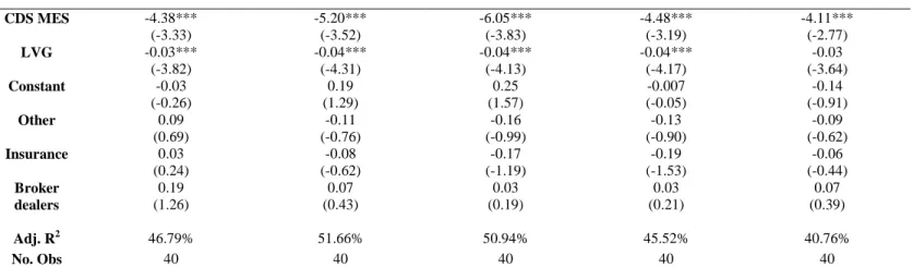
As final evidence, Table 8 provides formal statistics for regressions of both cds MES
based on cds returns (Panel A) or cds spread changes (Panel B) on realized equity returns during the same periods as Table 7. The results are quite strong with both cds MES and
leverage coming in at very high significant levels with adjustedR2s of 50% or higher using cds returns (and 30% plus using cds spread changes). The important point is that the systemic risk measures prior to the crisis have important information for which firms might run into trouble, and, therefore, by inference should, according to the optimal policy, be taxed to induce them to reduce their systemic risk. While cds MES seems especially useful prior to the start of the crisis, it is an open question that this will continue in the future with all the government guarantees now in place.
5
Related Literature on Measuring Systemic Risk
A number of recent papers have derived measures of systemic risk, mostly related to the financial crisis of 2007-2009. These papers can broadly be separated into two categories, one based on a structural approach using contingent claims analysis of the financial institution’s assets and the other on a reduced form approach focusing on the tail behavior of financial institutions’ asset returns. Consistent with the intuition provided in Section 2, all these approaches have the common feature of treating systemic risk in a portfolio context in which the portfolio is the financial sector, and individual assets are the financial institutions. As shown in Section 2 and argued in Section 3.1 above, the key variable must be the comovement between financial firms when the system as a whole is distressed.
With respect to contingent claims analysis, Lehar (2005) estimates the dynamics between financial institution’s assets using stock market data and a Merton model of bank liabilities. For different periods and countries, Lehar then measures the regulator’s total liability (if creditor were to be bailed out) and the contribution of each institution to this liability. Gray, Merton, and Bodie (2008) also use a contingent claims approach to provide an overall way of measuring systemic risk across different sectors and countries. Gray and Jobst (2009) apply the methodology to the current financial crisis, and quantify the largest institutions’ contributions to systemic risk in this crisis.
the strong assumptions that need to be made about the liability structure of the financial institutions. As an alternative, some researchers have used market data to back out reduced-form measures of systemic risk. For example, Huang, Zhou and Zhu (2009) use data on credit default swaps (CDS) of financial firms and stock return correlations across these firms to estimate expected credit losses above a given share of the financial sector’s total liabilities. Similarly, Adrian and Brunnermeier (2009) measure the financial sector’s Value at Risk (VaR) given that a bank has had a VaR loss, which they denote CoVaR, using quantile regressions. Their measure uses data on market equity and book value of the debt to construct the underlying asset returns.
Tarashev, Borio and Tsatsaronis (2009) present a game-theoretic formulation that also provides a possible allocation of capital charge to each institution based on its systemic importance. Farhi and Tirole (2009) model collective moral hazard and systemic bailouts. Finally, Segoviano and Goodhart (2009) also view the financial sector as a portfolio of indi-vidual financial firms, and look at how indiindi-vidual firms contribute to the potential distress of the system by using the CDSs of these firms within a multivariate setting.
Compared to these papers, our contribution is to build an explicit bridge between the structural and reduced-form approaches. On the one hand, we build a structural (albeit simple) model that provides the systemic contribution of each financial institution under reasonable assumptions. On the other hand, this systemic contribution can be written in terms of observables common to the reduced form approaches. Thus, systemic risk can be estimated using standard techniques and market data, as we illustrated for the financial crisis of 2007-2009.
6
Conclusion
Current financial regulations seek to limit each institution’s risk. Unless the external costs of systemic risk are internalized by each financial institution, the institution will have the incentive to take risks that are borne by all. An illustration is the current crisis in which