On Understanding Big Data Impacts
in Remotely Sensed Image Classification
using Support Vector Machine Methods
Gabriele Cavallaro,
Student Member, IEEE,
Morris Riedel,
Senior Member, IEEE,
Matthias Richerzhagen, J´on Atli Benediktsson,
Fellow, IEEE,
and Antonio Plaza,
Fellow, IEEE,
Abstract—Owing to the recent development of sensor reso-lutions on-board different Earth observation platforms, remote sensing is an important source of information for mapping and monitoring natural and man-made land covers. Of particular importance is the increasing amounts of available hyperspectral data originating from airborne and satellite sensors such as AVIRIS, HyMap, and Hyperion with very high spectral reso-lution (i.e., high number of spectral channels) containing rich information for a wide range of applications. A relevant example is the separation of different types of land cover classes using this data in order to understand for example impacts of natural disasters or changing of city buildings over time. More recently, such increases in the data volume, velocity, and variety of data contributed to the term “big data” that stands for challenges shared with many other scientific disciplines. On the one hand the amount of available data is increasing in a way that raises the demand for automatic data analysis elements since many of the available data collections are massively underutilized lacking experts for manual investigation. On the other hand, proven statistical methods (e.g.,, dimensionality reduction) driven by manual approaches have a significant impact in reducing the amount of “big data” towards smaller “smart data” contributing to the more recently used terms data value and veracity (i.e., less noise, lower dimensions that capture the most important information). This paper aims to take stock of which proven statistical data mining methods in remote sensing are used to contribute to “smart data” analysis processes in the light of possible automation as well as scalable and parallel processing techniques. We focus on parallel support vector machines (SVMs) as one of the best out-of-the-box classification methods.
Index Terms—Big Data; high performance computing (HPC); parallel processing; smart data; image classification; support vector machines (SVMs); data mining; spatial analysis;
I. INTRODUCTION
Recent advances in remote sensor and computer technology are substituting the traditional sources and collection methods
This research was supported by EU FP7 Theme Space project North State. The authors would like to thank Otto Buechner in particular and the JUDGE team at JSC in general.
G. Cavallaro is with the Faculty of Electrical and Computer Engi-neering, University of Iceland, Reykjavik 101, Iceland (e-mail: [email protected]).
M. Riedel is with the Juelich Supercomputing Centre, Germany and Uni-versity of Iceland, Reykjavik 101, Iceland (e-mail: [email protected]).
M. Richerzhagen is with the Juelich Supercomputing Centre, D-52425 Juelich, Germany (e-mail: [email protected]).
J. A. Benediktsson is with the Engineering Research Institute, University of Iceland, Reykjavik 107, Iceland (e-mail: [email protected]).
A. Plaza is with the Hyperspectral Computing Laboratory, Department of Technology of Computers and Communications, University of Extremadura, Ca´ceres 10071, Spain (e-mail: [email protected]).
of data, by revolutionizing the way remotely sensed data is acquired, managed and analyzed. The term remote sensing [1] refers to the science of measuring, analysing and interpreting information about a scene (or specific object) acquired by sensors mounted on board the different platforms for Earth and planetary observation.
Remote sensing instruments measure electromagnetic radia-tion energy at different wavelengths reflected or emitted by the Earth and its environment [2], which can be influenced by the radiation source, interaction of the energy with surface materi-als, and the passage of the energy through the atmosphere. The interactions of the energy with surface materials can change the direction, intensity, wavelength content, and polarization of electromagnetic radiation. The nature of these changes is dependent on the chemical make-up and physical structure of the material, exposed to the electromagnetic radiation, and can be used to provide major clues to the characteristics of the investigated objects.
The deployment of latest-generation sensor instruments on board both terrestrial and planetary platforms provides a nearly continual stream of high-dimensional and high-resolution data. More recently, such increases in the data volume, velocity, and variety of data contributed to the term“big data” that stands for challenges shared with many other scientific disciplines. In the context of remote sensing, sources and instruments currently available for Earth observation [3], generate different types of airborne or satellite images with different resolutions (i.e., spatial resolution, spectral resolution, and temporal res-olution). Hyperspectral remote sensors available from latest generation instruments, have substantially increased their spec-tral, spatial and temporal resolutions. In order to provide one example, the Airborne Visible/Infrared Imaging Spectrometer (AVIRIS) [4] is a 224-channel imaging spectrometer with approximately 10 nm spectral resolution covering the 0.4 to 2.5 µm spectral range, and it acquires reflected light of an area from2 km to12 kmwith a spatial resolution of 20m.
The availability of the aforementioned pieces of informa-tion, that we refer to concretely as“big data”in this contribu-tion, raises a demand forsmart data analytics techniquessuch as image processing, automatic classification, multitemporal processing and data fusion. In order to scale with the amount of available data, parallelization techniques are proposed in order to significantly accelerate the computations.
Parallelization techniques are typical implemented with two basic principles: (a) high throughput computing (HTC)
and (b) high performance computing (HPC). While low-cost systems such as commodity clusters in HTC or high-end supercomputers with good interconnects in HPC offer good scalability, parallel approaches are often complex to use especially for remote sensing domain scientists that are used to serial environments like Matlab or R. Also, in several cases, the need for parallel and scalable data processing can be reduced in the sense that “big data”can often be reduced to so-called “smart data” with less volume. This is possible by using less number of dimensions after applying statistical data mining such as principle component analysis (PCA) [5]. Our contribution will therefore critically review available parallelization techniques based on the emerging high num-ber of “big data stacks”, while not loosing sight of some traditional approaches known in HPC since decades. This will include several technical factors such as free and open technology availability, scalability of the solution, and specific algorithm suitability. This paper addresses those factors while analyzing data from one particular case study using Support Vector Machines (SVMs) [6] as one of the best out-of-the-box methods. In order to overcome the limitations of the wide variety of traditional serial SVM data analysis tools, we survey
and apply existing open source SVM tools for “big data
analytics” that take advantage of parallelization techniques. Efficiency benefits for the application domain problem are evaluated such as a lower time to solution or speed-ups obtained while building a data model.
Also, various other factors are discussed throughout this paper that influence the effectiveness and usefulness of so-called “big data analytics” solutions. The amount of time that domain-specific remote sensing scientists have to invest to manually work on datasets (e.g., apply feature extraction and selection methods) is important to consider. One of the funda-mental goals of“big data analytics”solutions is to support the manual time consuming data analysis process with automatic or semi-automatic solutions that are able to scale with the increasing high number of available scientific datasets. This gained momentum since the number of open datasets are increasing, but the number of domain-specific scientists stay rather constant over time. But in particular within scientific and engineering application domains, the manual contribution of the scientists remain often necessary, for example, a multi-class multi-classification problem may require different algorithms in order to improve the classification accuracy that is one of its major goals. This contribution will thus consider a classic pattern recognition approach based on the combination of feature extraction/selection and feature enhancement (i.e., spatial and neighbourhood analysis) methods.
This paper is structured as follows. After the introduction into the problem domain, Section 2 motivates our study and provides necessary background about the concrete scientific application problem and its required methods. Section 3 sur-veys related work in the field, while Section 4 offers the reader a thorough technology analysis in the light of the raised demands from the application problem. The findings in terms of technology are then evaluated in the context of a concrete scientific case study in Section 5, while this paper ends with some concluding remarks.
II. MOTIVATION
A. Remote Sensing Classification Application Case Study Our motivation is driven by the needs of a specific remote sensing application that raises the demand for technologies that are scalable with respect to“big data”. One of the main purposes of satellite remote sensing is to interpret the observed data and classify meaningful features or classes of land cover types. In hyperspectral remote sensing, images are acquired with hundreds of channels over contiguous wavelength bands, providing measurements that we consider as concrete “big data”in this paper. The reasoning include not only large data volume, but also a large number of dimensions (i.e., spectral bands).
Supervised classification is the essential technique used for extracting quantitative information from remotely sensed data such as the aforementioned hyperspectral images. It consists of learning from a training set of examples (hyperspectral data with class labels attached) and then generalize to find the class labels of hyperspectral data outside the training set. The high number of spectral bands can be handled by successful classifiers [7] and they can be useful for a wide variety of applications including: land-use and land-cover mapping, crop monitoring, forest applications, urban development, mapping, tracking, and risk management.
The SVM method provides an effective way to perform supervised classification of hyperspectral images [8]. SVMs have often been found to be more effective in terms of classification accuracies, computational time and stability to parameter settings than other widely used classifiers (i.e., maximum likelihood [9], K-nn [10] and the RBF neural networks [11]). Furthermore, SVMs appear to be especially advantageous in the presence of heterogeneous classes for which only few training samples are available. A key feature of the SVM supervised classification method is its ability to use high-dimensional data without the usual recourse to a feature selection step in order to reduce the dimensionality of the data. This is possible due to the integration of feature extraction and regularization elements within its learning process that is separately required in other algorithms.
But as a conventional classifier, SVMs use hyperspectral images based on its spectral information alone and do not con-sider the spatial information (dependencies of adjacent pixels). Additionally, hyperspectral data remains a challenge because of the data volume including hundreds of bands affected by redundancy and noise and the increasing number of labeled samples for training. The latter is problematic as SVMs badly scale with the number of samples [12]. For instance, spatial information can provide additional information related to the shape and size of different structures [13], which generally leads to better classification accuracies and classification maps. Hence, problems arise when all of the above-mentioned methods require fast and highly scalable solutions for realistic hyperspectral image analysis applications (e.g., analysis that is able to provide a response in real- or near-real-time). Our motivational case study thus requires a fast SVM solution for classification that is able to scale large remote sensing datasets and offers high accuracy with feature extraction methods.
B. Big Data Tools and Techniques
The term“big data”and its related term“big data analyt-ics” are often quoted in public literature such as in Mayer-Schoenberger et al. [14] or in the context of commercial data analysis (e.g., recommender systems using collaborative filtering techniques or association rule mining to understand customer buying habits and product placements). One of our motivational elements is therefore the observed fact that data mining tasks, originating from the scientific and engineering domain, raise the demand for so-called “scientific big data analytics”. This term aims to express that many techniques and algorithms commonly used in science and engineering problems are different to many of the aforementioned com-mercial data mining approaches. Evidence for this fact is given in many often quoted “success stories” like the Google Flu prediction published by Ginsburg et al. [15], while often little is known about their scientific shortcomings in such cases with respect to causality as published by Lazer et al. [16].
Given the momentum about “big data” activities driven
by success stories from Google and other commercial cases,
a wide variety of so-called “big data stacks” have been
developed. Examples include HTC-driven implementations adopting the “map-reduce paradigm” [17] such as the open source Apache Hadoop [18], which in turn lays the foundation for large machine learning frameworks like Apache Mahout [19] or individual algorithm implementations on top of it (e.g., Twister and parallel SVMs [20]). More recently, the machine learning library MLlib of Apache Spark [21] also gained momentum such as solutions based on Python like scikit-learn [22].
Our motivation is therefore to investigate those emerging stacks that claim to support parallel and scalable data mining or machine learning in order to take advantage of“big data”. Being driven by our concrete scientific case study in remote sensing, we would like to find out which of those “big data stacks”are suitable for our problem domain while not loosing sight of more traditional feasible approaches known from the field of HPC. Although HPC is driven by demands of the simulation sciences, based on efficient numerical methods and known physical laws, some of those applications raise equally challenging requirements to the processing environments as it is the case for our given remote sensing problem domain.
Despite the many possible characteristics of HPC environ-ments and the more recent “big data stacks”, one element of motivation in our study is driven by three simple criteria that are as follows. The first criteria is about the “(i) open and free availability of technology” in order to enable open and reproducable scientific analysis [23] compared to closed source or commercial license-based products of vendors. The criteria “(ii) technical feasibility” reviews capabilities such as scalability and parallelization approaches, including the maturity, deployments, and usability of tools and techniques. The third criteria “(iii) suitability of algorithms” reflects on our key requirement raised from the application domain-specific problem of using SVMs for classification of remote sensing images that in turn focusses our study on a concrete and specific “big data”problem to solve.
C. Support Vector Machines and Classification
The method we have choosen to perform image
classification is the well-known SVM [24], which is one of the most powerful classification and regression tools today. The general idea of SVMs lies on separating training samples which belong to different classes by tracing maximum margin hyperplanes in the space where the samples are mapped. Hence, SVMs only demands training samples close to the class boundary, it is thus capable of handling high dimensional data even if a small number of training samples is available. Our problem domain is a multi-class classification problem and SVMs solve this problem with the following given n input data instances (i.e., labelled training data):
Training set T = (x1, y1), ...,(xn, yn)
SVMs were originally introduced to solve linear classifica-tion problems. In order to generalize them to non-linear deci-sion functions, i.e., more complex classes that are not linearly separable in the original feature space, the so-called kernel trick can be taken into account [25]. A kernel-based SVM method maps input data instances into a high-dimensional feature space with a non-linear mapping function Φ (i.e., Gaussian radial basis function) and then performs linear clas-sification in this high-dimensional feature space. This mapping in accordance with Cover’s theorem [26] guarantees that the transformed data instances are more likely to be linearly seperable. The mapped data instances belonging to different classes (i.e., multi-class) are separated by tracing maximum margin (decision) hyperplanes in this higher dimensional space. Since maximizing the distance of data instances to the optimal decision hyperplane is equivalent to minimizing the norm of the weight w, SVMs solve the following constraint optimization problem: min w,ξi,b ( 1 2 w 2 +CX i ξi ) (1) subject to: yi(hφ(xi),wi+b)≥1−ξi ∀i= 1, ..., n (2) ξi≥0 ∀i= 1, ..., n (3)
Data instances with labelled data have label yi, while the
ξi are positive slack variables allowing to deal with permitted
errors. SVMs use the important generalization parameter C. which controls the shape of the solution of the decision boundary. Thus it affects the generalization capability of the SVMs, e.g., a large value of C might cause an over-fitting to the training data. Equation (1) can be transformed in its dual problem that in turn can be solved using quadratic programming (qp) mechanisms. The learning model selection in terms of choosing the right values for C andξiis performed
using cross-validation techniques. The sensitivity to the choice of the kernel and regularization parameters can be considered as the most important disadvantages of SVM. A complete introduction to SVMs is out of scope and we refer to C. Cortes et al. [24] for more technical details.
III. RELATEDWORK
The use of parallel and scalable techniques within the field of remote sensing is not new and we survey previous approaches as part of this section. In contrast to those previous approaches, our current study focuses much more on three characteristica: (a) “big data” and statistical techniques to transform“big data”into“smart data”and (b) broader view on parallelization methods including not only HPC methods, but also HTC such as map-reduce-based implementations, and (c) open data science enabling reproducability of results.
The major source for using parallel and scalable techniques in remote sensing is a book by Plaza et al. [27] that particularly focuses more on HPC techniques and mentions less HTC approaches. As the book was written in 2008, several of its elements are rather outdated and as a consequence we started the study reported in this paper in order to solve remote sensing problems with the power of HPC systems available in 2015. Our three mentioned general characteristica from above (a), (b), and (c) are rarely covered in the book, and SVMs in particular are only mentioned in the context of “Computer Architectures for Multimedia and Video Analysis”[27].
A more focussed survey of SVM parallelization approaches in the context of remote sensing is as follows. In [12], Munoz-Mari et al. discusses the use of SVMs for hyperspectral multi-class image multi-classification highlighting also previous attempts for parallelization in this regard. The author evaluates a massively-parallel SVM implementation based on the incom-plete Cholesky factorization and load balancing as well as parallelization principles that take advantage of the traditional Master-Worker decomposition quite well known in HPC. The evaluations mentioned in the paper are performed on two supercomputers in Spain and USA, but in contrast to our case study used not only a different SVM implementation, but also other feature extraction approaches. The paper also discusses not directly classification accuracies after training the model with parallel and scalable SVM methods, while in this paper we list obtained accuracies in the cases of raw data (w/o applying feature extraction) and processed data (with applying features extraction) in order to point out their trade-offs.
More recently, in 2011, Plaza et al. describes in [28] the use of HPC techniques for analysing hyperspectral remote sensing problems with a focus on commodity architectures and specialized hardware such as Field Programmable Gate Arrays (FPGAs) and commodity Graphic Processing Units (GPUs). The paper describes parallel and scalable approaches of the hyperspectral unmixing chain and, in contrast to our given case study, not only thus solves another problem with other techniques (i.e., not SVMs), but also uses different datasets and hardware technology. The results around GPUs however inspired us to include them in our technology review in order to explore available stable and mature implementations.
All aforementioned implementations have been unfortu-nately not actively maintained and are thus outdated or not openly available to solve our given scientific case study prob-lem today. To the best of our knowledge there are no major other approaches in the field of remote sensing classification using parallel and scalable methods with SVMs.
IV. TECHNOLOGYREVIEW ANDANALYSIS
There is a high number of technologies that appear to be suitable as solutions in our problem space with a particular focus on SVMs. But closer investigations of the functionality of broadly known tools or often used techniques reveal quite surprising facts in the light of the presented scientific appli-cation case study. One goal of the technology review in this section is therefore not only to inform the reader about general availability, but also to filter tools and techniques in the light of their suitability for a concrete “big data”problem.
A. Overview of Serial Technologies
Traditional data analysis has taken advantage of well es-tablished and mature tools such as those listed in Table I. The simplicity combined with state of the art performance on many learning problems (classification, regression, and novelty detection) has contributed to the popularity of the SVM.
The survey results show that all of the known technolo-gies, such as open source machine learning toolkits (i.e., scikit-learn) and programming languages (i.e., Matlab and R), support a multi-class SVM implementation. The majority of them are wrappers of the de-facto standard implementation of LibSVM [29], the most popular open source machine learning library [29], developed at the National Taiwan University and written in C++ though with a C API.
For example, scikit-learn [30] is an open source machine learning library largely written in Python, with some core algorithms written in Cython to achieve performance. Support vector machines are implemented by a Cython wrapper around LibSVM. R [31] is an extremely popular open source statistical software platform, which provides a wide variety of statistical methods. The implementation of SVM in R is included in the e1071 package [32]. Matlab [33] is a multi-paradigm numerical computing environment widely used in academic and research institutions as well as industrial enterprises. Many enhancement are applied to the C version of the LibSVM library to speed up Matlab usage. Pre-compiled MEX func-tions Matlab that wrap around the LibSVM C library are widely available. In the remote sensing domain, there are many commercial software tools with GUIs that offer many functions for the analysis and visualization of scientific data and imagery. ERDAS [34] and ENVI [35] are placed in the top of the heap, both specialized software for the analysis of hyperspectral data, and they included the SVM classifier.
The described tools, that we refer to as“serial tools”when using“big data”in terms of a very high number of samples or high number of dimensions, can lead to challenging problems during the data analysis. For example, already while loading such datasets into some of the listed tools in Table I, we observed serious waiting times or even memory problems on desktop machines. In some cases, even before processing time, the necessary pre-processing time took quite a substantial time (e.g., applying feature extraction algorithm on the input data). Despite the fact that the model building process (i.e., training and testing a model) is still possible in several tools, the waiting time became unfeasible long. This is the case when applying cross-validation, which is necessary for model
selection but which can take a significant amount of time using tools like Matlab. Selected drawbacks of so-called serial desktop approaches have been listed above, but one should also mention that modern desktop computers and laptops becoming increasingly multi-core and as such also perform better than, for example, using just one naturally serial core on a supercomputer. This impact of multi-core desktop and laptop systems will be one element of our study that we take into account when performing evaluations. But even those desktop solutions have limitations in memory and available cores and as such parallel and scalable approaches on large-scale HPC-oriented machines or HTC-driven distributed systems bear the chance to overcome those limitations.
TABLE I: Overview of selected common serial tools and their analysis.
Technology Analysis
R Statistical Computing SVMs (multi-class) Matlab SVMs (multi-class) LibSVM SVMs (multi-class) scikit-learn SVMs (multi-class) Erdas image SVMs (multi-class)
Envi SVMs (multi-class)
Weka SVMs (multi-class)
B. Overview of Parallel Technology Approaches
Given the momentum of“big data”at the time of writing, there is a wide variety of technologies that aim to support“big data analytics”in general and the analysis of large quantities of data in particular. Table II offers a summary overview of the performed analysis listing technologies with a particular focus on investigating parallelization capabilities in order to be able to scale for large datasets. The analysis further takes into account the required SVM methodology details such as the aforementioned multi-class classification capability or support for non-linear models that are required by the scientific case study.
One of the most known approaches for “big data
ana-lytics” in terms of scalable machine learning is the Apache Mahout software [36]. It is based on parallel map-reduce and the Apache Hadoop 1.0 [37] implementation, but is in the transition of taking advantage of Apache Spark [38] as a underlying platform in order to enable more functionalities such as a more flexible parallel execution model. At the time of writing, Apache Mahout version 0.9 offers no parallel SVM implementation in the official release and thus it is not a technology of choice for the scientific case study in this contribution.
A more recent approach for“big data analytics”including smart parallelization techniques is the comprehensive plat-form Apache Spark [38]. Experience from various sources
suggests major improvements in performance, e.g. “Spark
can outperform Hadoop by 10x in iterative machine learn-ing jobs” [39]. Beside the support for SQL, streaming, and graph-based problems, the Spark MLlib library offers several
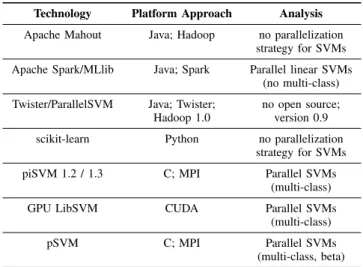
TABLE II: Overview of known parallel tools and their analy-sis.
Technology Platform Approach Analysis
Apache Mahout Java; Hadoop no parallelization strategy for SVMs Apache Spark/MLlib Java; Spark Parallel linear SVMs
(no multi-class) Twister/ParallelSVM Java; Twister; no open source;
Hadoop 1.0 version 0.9
scikit-learn Python no parallelization
strategy for SVMs
piSVM 1.2 / 1.3 C; MPI Parallel SVMs
(multi-class)
GPU LibSVM CUDA Parallel SVMs
(multi-class)
pSVM C; MPI Parallel SVMs
(multi-class, beta)
implementations for parallel and scalable machine methods. A deeper investigation in light of the scientific case study however reveals that version MLlib 1.1 only support linear SVMs and as such this implementation is not a technology of choice given the specific problem space in this contribution.
Another parallel implementation is open source and de-scribed by Zhu et al. in [40]. Our analysis of this implemen-tation based on Message Passing Interface (MPI) reveals that it is an unstable beta release that is also slightly outdated. The pSVM is thus not a candidate tool we can work with in the context of the scientific case study. Our analysis reveals only three different applicable approaches that will be more thoroughly discussed in the next section.
C. Applicable Parallel Technology Approaches
The analysis of parallel technology provides three applica-ble approaches as shown in Taapplica-ble III, because also scalability of technologies is a concern that is taken into account. Deeper analysis reveals further facts towards the selection of one technology to be used in the problem domain with respect to their usability and stability in practice.
All three applicable techniques in Table III are internally based on the serial libSVM tool that in turn ensures a stable functionality of the SVM methodology. Their parallelization approaches however vary significantly in terms of stability and usability that are both a major concern in parallel and distributed systems.
TABLE III: Suitable parallel tools after their deeper analysis.
Technology Platform Approach Deeper Analysis
Twister/ParallelSVM Java; Twister; no real release; Hadoop 1.0 complex software stack piSVM 1.2 / 1.3 C; MPI Stable, but not fully
scalable
GPU LibSVM CUDA/Nvidia hard to program;
The parallel SVM based on iterative map-reduce with Twister has been used and is the most scalable version for “big data” being not limited by the size of one particular physical machine. As this approach is based on Hadoop and map-reduce, as least theoretically more and more compute nodes could be added to achieve a speed-up. But there is no official release for the parallel SVM implementation on top of Twister and thus the source can be only obtained by contacting the author of its scientific paper [41]. Beside the fact that this is not inline with the aforementioned open data science thorough investigations in applying this approach in the given problem domain shows that its stability and usability could be improved. One reason is that the Twister version is based on Hadoop 1.0 and that several scheduling tricks need to be applied before using it. Another reason is the dependency on a messaging system (for iterative map-reduce) that further adds to the complexity (and thus stability) of the whole stack.
The analysis of piSVM 1.2 and its more recent version 1.3 revealed a very stable version of the implementation not only because it is based on libSVM, but also since it takes advantage of the mature MPI standard. Its use of scheduling (i.e., jobscript) by this technology approach is inline with large computing centres and the source itself is open source and freely available [42]. The only drawbacks have been scalability limits that requires certain tunings to the piSVM code that have been applied thus making this technology at the time of writing the best openly available and scalable solution for our problem domain. We focus here on selected tunings of this technology that in theory is only limited with respect to the number of cores available in the corresponding choosen cluster with an MPI environment. One of the tunings for speed-up improvements was the change of loops and single MPI calls to a more wider use of efficient MPI collective operations. Another tuning is the use of a better domain decomposition design in the parallelization to scale with our dataset (e.g., using 52 classes, more than 32 cores, etc.).
In practice, the particular problem domain given by the scientific case study in this paper reveals that large number of cores are typically not needed and thus one can assume that modern clusters with MPI offer the required number of cores as small to medium computing clouds. Furthermore chooosing this technology is not necessarily a problem for big data as computing centres often use parallel file systems with massive amount of storage connected to it. One of the reasons of this fact is that the modern community in scientific computing and the inputs and outputs of simulations often require also huge amount of storage and thus this field has dealt traditionally very long with emerging “big data”including today.
Finally, one of the most interesting emerging implementa-tions that bears a lot of potential is the GPU LibSVM [43] as GPUs gain tremendous momentum on the hardware and software side in the parallelization communities. At the time of writing, our analysis has shown some limitations in practically using this implementation, also because it has dependencies to the proprietary Compute Unified Device Architecture (CUDA) technolgy stack. It is thus not straightforward to use this library to implement our case study, but we mark this technology as a distinct candidate to work with in future work.
V. SCIENTIFICCASE ANDEVALUATION
One of the main challenges that occur with hyperspectral images is related to the design of the classification framework. In this section we describe the supervised classification chain for a serial processing environment based on spectral-spatial analysis and evaluate in context potential improvements and results when applying parallel and scalable techniques.
A. Applied Statistical Methods in Remote Sensing
The implicit dimensionality of hyperspectral images is responsible for important limitations in the application of supervised classifiers. The huge amount of data often requires a reduction of features to make classification flexible and computationally efficient. Moreover, the limited availability of training samples and the complex data structure imposes further restrictions to the full data exploitation within a hyper-dimensional space (Hughes phenomenon [44]). In addition, the high correlation between neighboring bands in hyperspectral data sets is responsible for redundancy, which strongly af-fects the performances of traditional supervised classification techniques. As a consequences, the application of feature selection and reduction techniques prior to the classification is recognized as critical to the improvement of the classification results. In the literature, several data mining techniques [45] have been developed to address this task. Different techniques can include supervised and unsupervised, parametric and nonparametric, linear and nonlinear methods, which all seek to identify the relevant informative reduced subspace (i.e., without losing significant information), where the separability of the classes is improved.
In this work, we adopt a classification chain which in-cludes one unsupervised and one supervised feature extrac-tion method. Despite the slight differences between the two approaches, since one works directly on the data and the other works with the support of reference samples, both approaches aim to select features that are consistent with the target concept. In unsupervised approaches the target concept is usually related to the innate structures of the data, and the main objective is usually to represent the data in a lower dimension space. In supervised approaches the target concept is related to class affiliation, and they are usually consid-ered for overcoming the Hughes phenomena and reducing the redundancy of hyperspectral data in order to improve classification accuracies.
B. Mathematical morphology in Remote Sensing
Recent efforts in the literature [46] have demonstrated that hyperspectral image classification can greatly benefit from an integrated framework in which both spatial-spectral in-formation are included into the analysis process. The spatial information provides an essential contribution to the under-standing of the remote sensing images, since it characterizes the sensed landscape in a complementary way with respect to the spectral signatures of the land covers. Spatial information can be coded as relations between neighboring pixels, patterns in the spatial domain (e.g.,, texture), spatial characteristics of regions (e.g.,, geometrical, morphological, textural measures),
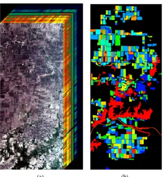
(a) (b)
Fig. 1: AVIRIS Indian Pines image cube representation (a) and ground reference (b)
structural relations in objects, or relational links between entities in the scene. From a general survey of techniques modeling the spatial information in remote sensing, one can notice that there are different approaches for extracting the spatial information and correspondent ways (with different levels of abstraction) for including the extracted information in the processing chain aiming at the classification of the image. An automatic analysis and interpretation of the characteris-tics of spatial information can be achieved by processing an image with a set of mathematical morphology operators. In this context, recently region-based filtering tools [47] (called connected operators) have received significant attention due to their effectiveness in both extracting spatial information and preserving the geometrical characteristics of the objects in images (i.e., borders of regions are not distorted since only an image is processed by merging its flat zones). Attribute filters [48] are a set of connected operators that are able to simplify a grayscale image according to an arbitrary measure (i.e., attribute), such as scale, shape and contrast.
Dalla Muraet al. [49], proposed self-dual attribute profiles (SDAPs) as a variant of Attribute Profiles (APs) [50] for the classification of very high geometrical resolution images. SDAPs are obtained by filtering a given grayscale image with attribute operators using a predicate with increasing threshold values. Cavallaroet al.in [51] proposed the extended self-dual attribute profiles (ESDAPs), as the application of SDAPs to hyperspectral data. An ESDAP is obtained by concatenating the SDAPs (i.e., based on one or more attributes) built on several feature components extracted by a reduction technique (i.e., KPCA) computed on the hyperspectral image.
C. Remote Sensing Data set
The experiments has been carried out on the Indian Pines AVIRIS dataset that is shown in Fig.1, which is publicly
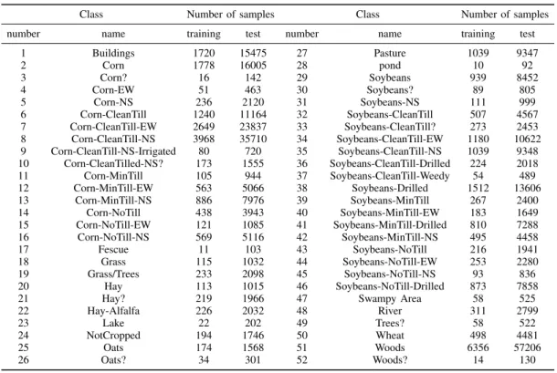
avail-able [52] and widely used for feature reduction and classifica-tion of hyperspectral images. The Indian Pine airborne data set was acquired in June 1992 over an agricultural site composed of agricultural fields with regular geometry and with a variety of crops. A small portion (145×145 pixels) of the original image has been extensively used as a benchmark image for comparing different classifiers. Here, however, we consider a larger portion, which consists of 1417×617 pixels and 200 spectral bands (20 bands with low Signal to Noise Ratio (SNR) were removed), with a spatial resolution of 20 m. From the 58 different land-cover classes available in the original ground-truth, 6 classes were discarded (classes with less than 100 samples). This data set represents a very challenging land-cover classification problem dominated by similar spectral classes and mixed pixels. Specifically, the discrimination of the major crops of the area (corn and soybeans) is very difficult since they were very early in their growth cycle (with only about 5% canopy cover), meaning that most of the scene pixels are highly mixed.
D. Classification Design
Many different processing configurations have been studied for remotely hyerspectral image classification including data transformation (e.g.,, for dimensionality reduction), feature extraction/selection, and spatial information analysis. Our sci-entific case in this paper considers two different classification scenarios, which are shown in Fig. 2:
1) Scenario with near real-time processing constraints. The hyperspectral data set is not manually analyzed, and a straightforward classification is performed.
2) Scenario without time processing constraints. A process-ing chain spatial-spectral analysis is manually applied in order to improve the effectiveness of a classifier. In both scenarios we assume that data correction activities such as sensor specification, geometric corrections, radiomet-ric calibrations were already performed [53]. A more detailed description for the different data analysis steps included in the classification chain shown in Fig. 2 is as follows:
• Dimensionality reduction: the first step consists of reduc-ing the dimensionality of the data to a subspace with the minimum loss of the original information. For such a task, the unsupervised Kernel Principal Component Analysis (KPCA) [54] technique is here considered. The KPCA is the non-linear version of PCA [5], and it is capable of dealing with the non-linearities of the data (i.e., it shares the same properties as the PCA but in a different space). The advantages of using KPCA instead of PCA is that
KPCA 90% ESDAP NWFE Train SVM
GroundTruth Train set Test set
SVM classifier Model 99% Data set (2) (1) Cross validation
more information is provided from the original data set since higher-order statistics is captured (i.e., due to an appropriate projection of the data onto another space).
• Spatial analysis: in the second step, spatial information
analysis is included in the process, since only the spectral information may not be able to accurately model spatial dependencies in the scene. The spatial analysis is here performed by ESDAP built on the features extracted by KPCA by using the area and standard deviation attributes. The area allow the extraction of objects based on their size, while the standard deviation can model the homogeneity of the pixels gray levels belonging to different regions. The thresholds are manually selected by a visual analysis of the scenes.
• Feature extraction: in the third step, a feature extraction method is included prior to classifier. In the literature [55], the Nonparametric Weighted Feature Extraction (NWFE) supervised method has been widely used to reduce the number of morphological features extracted by the morphological analysis (ESDAP). The NWFE technique is an efficient algorithm for high dimensional multi-class pattern recognition problems. Since NWFE is based on a nonparametric extension of scatter matrices (i.e., between-class and within-class), the algorithm is able to extract a desired number of features (higher than the number of classes) and can work well even for data that are not Gaussianly distributed [56].
E. Experimental Setup and Results
The serial experiments were implemented in MATLAB on a computer having Intel(R) Core (TM) i7-4710HQ CPU 2.50 GHz and 16 GB of memory. The CPU processing time re-ported in Table VI are related to data analysis and classification (training and testing) steps using this experimental setup. In the data analysis side of the processing chain, the ESDAP is the step which requires most of the time. The ESDAP are computed by using C++ Milena library [57] and an adaptation of the code for the Inclusion tree provided in the MegaWave2 toolbox [58] (more about the algorithm and the processing information can be found in [59]).
TABLE IV: Serial case for scenario 1: 10-fold grid search cross-validation. The accuracies and the computation times (in brackets) are reported for each combination of the regulariza-tion and kernel parameters. The best accuracy is marked in bold and indicates the optimal C and kernel γ used in the training phase. The overall time is 4.47×10³min (3 days).
γ/ C 1 10 100 1000 10000 2 27.30 (109.78) 34.59 (124.46) 39.05 (107.85) 37.38 (116.29) 37.20 (121.51) 4 29.24 (98.18) 37.75 (85.31) 38.91 (113.87) 38.36 (119.12) 38.36 (118.98) 8 31.31 (109.95) 39.68(118.28) 39.06 (112.99) 39.06 (190.72) 39.06 (872.27) 16 33.37 (126.14) 39.46 (171.11) 39.19 (206.66) 39.19 (181.82) 39.19 (146.98) 32 34.61 (179.04) 38.37 (202.30) 38.37 (231.10) 38.37 (240.36) 38.37 (278.02)
When comparing the two phase feature extractions, the first step (KPCA) requires more time than the second step (NWFE) since the former has to deal with the dimension and the com-plexity of the hyperspectral data set. For the KPCA method,
TABLE V: Serial case for scenario 2: 10-fold grid search cross-validation. The accuracies and the computation times (in brackets) are reported for each combination of the regulariza-tion and kernel parameters. The best accuracy is marked in bold and indicates the optimal C and kernel γ used in the training phase. The overall time is 529.55min.
γ/ C 1 10 100 1000 10000 2 48.90 (18.81) 65.01 (19.57) 73.21 (20.11) 75.55 (22.53) 74.42 (21.21) 4 57.53 (16.82) 70.74 (13.94) 75.94 (13.53) 76.04 (14.04) 74.06 (15.55) 8 64.18 (18.30) 74.45 (15.04) 77.00(14.41) 75.78 (14.65) 74.58 (14.92) 16 68.37 (23.21) 76.20 (21.88) 76.51 (20.69) 75.32 (19.60) 74.72 (19.66) 32 70.17 (34.45) 75.48 (34.76) 74.88 (34.05) 74.08 (34.03) 73.84 (38.78)
TABLE VI: Serial case CPU processing time (in minutes).
kpca esdap nwfe 10x CSV Training Test Total (1) Scenario 0 0 0 4.47×10³ 10,45 71,08 4.55×10³
(2) Scenario 5 15.38 1 529.55 1.37 23.25 575.55
the kernel function adopted is Gaussian kernel and the param-eter is estimated as the mean value of the distance between each samples. The Kernel Matrix is computed by randomly selecting 500 samples from the total number of pixels present in the image (i.e., in order to perform the transformation in an acceptable processing time). The hyperspectral data set is reduced into a subspace of feature components, where the first features with cumulative variance of more than 90% are kept. For the NWFE approach, the Leave-One-Out Covariance (LOOC) estimator is applied to regularize the within-class scatter matrix and the mixing parameter β [60] is fixed at 0.5. The resulting first features with cumulative variance of more than 99% are kept for the subsequent classification step. For the classification, the number of training and test samples are reported in Table X, where the training set was randomly selected by using 10% of the labeled samples from each class. For the classifier, the Gaussian radial basis function (RBF) kernel is adopted. The values of C andγ, regularization parameter and width of the RBF, respectively, are optimized using a 10-fold cross-validation procedure. The grid search consists of a discrete set of 5 values for both parameters, i.e., C=[1,10,100,1000,10000] and γ=[2,4,8,16,32]. Looking at the CPU processing times for the cross-validation, training and test, it can be noticed that in the second scenario the times are drastically reduced. This is due to the application of data analysis pre-processing, which reduces the complexity (dimension and noise) of the “big data” and enhances its spectral and spatial information by producing a“smart data”, which is more simple to be processed by the classifier. This is confirmed by the classification results shown in Table VII
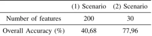
TABLE VII: Classification accuracies for the raw spectral data and for the data analyzed with the proposed scheme in percentage.
(1) Scenario (2) Scenario
Number of features 200 30
which shown an improvement of more than 37% in terms of overall accuracy experimented in the second scenario. In the literature [61] and [62], classification results for the same data set can be found. Although the data analysis is an important but also critical step in the process of converting the “big data”into user-required products we refer to as“smart data”, the process is not straightforward and it requires time (manual work) and enough expert knowledge.
The next step in our evaluation consists of analyzing the same dataset with parallelization techniques in order to find out whether we are able to achieve a speed-up of cross-validation, training and test periods by keeping the respective accuracies shown in Table VII. The parallel experiments have been implemented using our optimized piSVM tool on the JUDGE supercomputer at the Juelich Supercomputing Centre with a number of 206 compute nodes IBM System x iDataPlex dx360 M3. Each compute node has 2 Intel Xeon X5650 (Westmere) 6-core processors with 2.66 GHz. The main memory is 96 GB and the fast interconnect is an Infiniband system that is used with the Partec MPI implementation in our case study. Used data sets, job scripts, data models, and results are available at [63], [64], [65], [66] and [67] in order to support reproducible open science.
We firstly discuss the speed-up achieved in the scenario (1) of satisfying a near real-time processing constraints meaning that the data is in itsraw form. As can be seen in Table IV, the cross-validation in the serial case is very computationally in-tensive. The reason is that the training-validation is performed
10 times for each of the 25 combinations of the C and γ
parameters. The total processing time is4.47×103min, which
is more than 3 days. Because each partition set is indepen-dent, the cross-validation performed in parallel can achieve a significant speed up, by reducing the overall processing time to 138.72 min using 80 cores as reported in Table VIII. As shown in Fig. 3(a), the training time in this scenario can be also reduced with the minimal training time of 0.55 min using 80 cores. When comparing this result with the serial training time listed in Table VI, we observe that we can thus significantly reduce the computing time from 10.45 min to 0.55 min. Finally, by using parallelization techniques, we have been able to also reduce the test time in this scenario to a minimal test time of 4.09 min using 80 cores as shown in Fig. 3 (b). The serial test time obtained by using Matlab is 71.08 min that in turn indicated a major speed-up when using parallelization techniques, in particular because the test set is also much larger than the training set. The impact of using parallelization techniques for large quantities of samples (aka “big data”) is thus much higher than in those with less training samples.
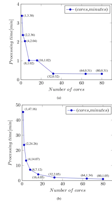
The question remains that time gains in the manual process of scenario (2) using feature extraction methods, thus lowering the demand for CPU processing, will outperform the speed-up gained by parallelization techniques. We study this particular question while discussing the speed-up results of the scenario (2) that do not raise any real-time requirements. As in the previous scenario, the most notable speed up is achieved in the cross-validation step. Its overall processing time is reduced to 35.54 min (see Table IX) using 80 cores, from the 529.55
min of the serial case (see Table V). As shown in Fig. 4 (a), the training time in scenario (2) can be also reduced to a minimal training time of 0.32 min using only 32 cores (i.e., no improvements are observed when increasing the number of cores). When comparing this result with the serial training time of scenario (2) listed in Table VI, we observe that we can just slightly reduce the 1.37 min to 0.32 min. As it was already the case with scenario (1), by using parallelization techniques, we have been able to also reduce the test time in this scenario to a minimal test time of 1.05 min using 80 cores as shown in Fig. 4 (b). The serial test time by using Matlab is 23.25 min and as it was already the case for the scenario (1), we also observe for scenario (2) a major speed-up when using parallelization techniques.
Our evaluation can be summarized with respect to speed-up of the training and testing process by not loosing sight the important measure of accuracies. For both scenario (1) and (2), using parallelization techniques, a speed-up is achieved by maintaining accuracy when using only a moderate number of cores (i.e., compared to those number of cores that are used in the simulation sciences). The majority of the results are also remarkable in the sense that we observe that we can just slightly reduce the 1.37 min to 0.32 min. Nevertheless, the majority of the results are also remarkable in the sense that CPU times below 1.00 min can be still considered as an “interactive experience”. This means it is possible to wait for the results when using parallel techniques while in the serial case a remote sensing scientists are rather tempted to perform other work thus interrupting the ordinary work session and thus reducing the productivity of the scientist.
We further evaluate the whole process chain of scenario (1) and (2) that we denote in Table VI as “Total” time. This time includes the time spent applying different feature extraction and selection techniques, but also the time for cross-validation, training and testing, respectively. In scenario (1), the serial approach in Matlab leads to a Total time of
4.55×10³ min (3 days) for the raw dataset not using any
feature extraction technique and by using parallelization this can be reduced to a Total time of only 143.36 min. In scenario (2), the serial approach requires a Total time of 575.55 min for the processed dataset taking already advantage of feature extraction techniques including also dimensionality reduction techniques (i.e., after applying KPCA for example). In the context of scenario (2), the parallelization techniques achieve a remarkable reduction leading to a Total time of 58.28 min. The parallelization benefit is mostly shown when performing model selection with n-fold cross validation compared to serial programs like Matlab. The added value for remote sensing scientists is thus that they can more easier and faster experiment with different feature extraction techniques and processing chains (cf. Fig. 2) that often bear the potential to increase the accuracy of the classifier.
VI. CONCLUSION
One of the reasons of this study was to understand whether parallelization techniques can overcome limitations observed in serial tools when working with emerging concrete examples of “big data”. This is particular interesting as traditionally serial tools could still work with datasets by applying feature extraction or selection techniques as well as subsequent dimen-sionality reductions or smart resampling (i.e., lower volumes of data). When working with larger quantities of data we have evaluated parallelization techniques in order to offer selected findings in the context of one specific challenging scientific case study dataset (i.e., concrete “big data”).
One conclusion from the technology reviews is that despite the availability of many parallelization techniques, just a very limited set of suitable parallel tools exist in the open source domain for our concrete problem space of using parallel SVMs. Even those we identified as being suitable and being open source, still required tuning (i.e., piSVM) or are not straightforward yet to use with common parallel hardware (i.e., GPU LibSVM for CUDA/Nvidia cards only). But we also observe a momentum in the parallelization community around GPUs that is affecting also other fields (e.g., machine learning, bioinformatics, deep learning, etc.) and therefore we consider the work on GPUs as a major element in directions of future work.
We conclude that, by using our tuned version of the piSVM implementation, in both scenarios (1) and (2), applying our parallelization techniques lead to significant speed-ups for the cross-validation and for each training and testing process. More notably, this is achieved by maintaining the same ac-curacy as achieved when performing the processes with serial tools. In the majority of cases, the minimal training and testing time was around one minute that still can be considered as an “interactive experience” thus enabling remote sensing scien-tists to easier and faster experiment with different techniques (e.g., applying quick parameter variations of feature extraction techniques).
We thus conclude that the Total time of the whole process can be significantly reduced by using parallelization methods making it still feasible to use even when feature extraction and selection techniques and spatial analysis methods are applied. We also conclude that the added value of using parallelization techniques for large quantities of samples and multiple cross-validation runs. (aka “big data”) is higher than in those with less training samples. It is still feasible to apply feature extraction techniques not only to increase the accuracy of a classifier and lower thus the data volume, but also to reduce the number of computing cycles needed since in many cases HPC processing time is costly. However, the inclusion of the spatial information analysis is essential for a proper exploitation of all the available informative components. ESDAP have proven to be an effective tool for the modeling of the different spatial characteristics and for providing additional informative features. With the achieved speed-ups it thus become feasible to approach other“big data”challenges in the remote sensing community, such as change over a city over decades that we currently outline as future work.
TABLE VIII: Parallel case (80 cores) for scenario 1: ten-fold grid search cross-validation. The accuracies and the computa-tion times (in brackets) are reported for each combinacomputa-tion of the regularization and kernel parameters. The best accuracy is marked in bold and indicates the optimal C and kernelγused in the training phase. The overall time is 138.72min.
γ/ C 1 10 100 1000 10000 2 27.26 (3.38) 34.49 (3.35) 39.16 (5.35) 37.56 (11.46) 37.57 (13.02) 4 29.12 (3.34) 37.58 (3.38) 38.91 (6.02) 38.43 (7.47) 38.43 (7.47) 8 31.24 (3.38) 39.77 (4.09) 39.14 (5.45) 39.14 (5.42) 39.14 (5.43) 16 33.36 (4.09) 39.61 (4.56) 39.25 (5.06) 39.25 (5.27) 39.25 (5.10) 32 34.61 (5.13) 38.37 (5.30) 38.36 (5.43) 38.36 (5.49) 38.36 (5.28)
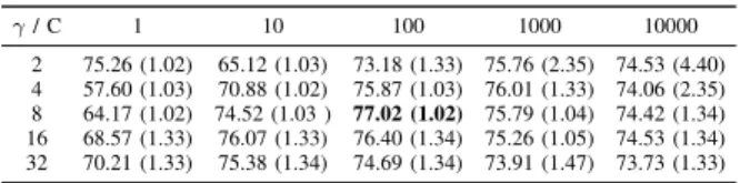
TABLE IX: Parallel case (80 cores) for scenario 2: ten-fold grid search cross-validation. The accuracies and the computa-tion times (in brackets) are reported for each combinacomputa-tion of the regularization and kernel parameters. The best accuracy is marked in bold and indicates the optimal C and kernelγused in the training phase. The overall time is 35.54min.
γ/ C 1 10 100 1000 10000 2 75.26 (1.02) 65.12 (1.03) 73.18 (1.33) 75.76 (2.35) 74.53 (4.40) 4 57.60 (1.03) 70.88 (1.02) 75.87 (1.03) 76.01 (1.33) 74.06 (2.35) 8 64.17 (1.02) 74.52 (1.03 ) 77.02 (1.02) 75.79 (1.04) 74.42 (1.34) 16 68.57 (1.33) 76.07 (1.33) 76.40 (1.34) 75.26 (1.05) 74.53 (1.34) 32 70.21 (1.33) 75.38 (1.34) 74.69 (1.34) 73.91 (1.47) 73.73 (1.33) REFERENCES
[1] C. F. W. S. Khorram, F. H. Koch and S. A. C. Nelson,Remote Sensing, 2012, vol. 7. [Online]. Available: http://www.springer.com/new+%26+ forthcoming+titles+%28default%29/book/978-1-4614-3102-2 [2] C. Elachi and J. Van Zyll,Introduction to the physics and techniques of
remote sensing. Hoboken, N.J: Wiley-Interscience, 2006.
[3] Q. Weng,Advances in environmental remote sensing : sensors, algo-rithms, and applications. Boca Raton: CRC Press, 2011.
[4] R. O. Green, M. L. Eastwood, C. M. Sarture, T. G. Chrien, M. Aronsson, B. J. Chippendale, J. A. Faust, B. E. Pavri, C. J. Chovit, M. Solis, M. R. Olah, and O. Williams, “Imaging spectroscopy and the airborne visible/infrared imaging spectrometer (aviris),”Remote Sensing of Environment, vol. 65, no. 3, pp. 227 – 248, 1998. [Online]. Available: http://www.sciencedirect.com/science/article/pii/S0034425798000649 [5] K. Fukunaga,Introduction to Statistical Pattern Recognition, (2nd ed.).
W. Rheinboldt, Ed. New York, NY, USA: Academic Press Professional, Inc., 1990, vol. 2.
[6] C. Cortes and V. Vapnik, “Support-vector networks,” Machine Learning, vol. 20, no. 3, pp. 273–297, 1995. [Online]. Available: http://dx.doi.org/10.1023/A%3A1022627411411
[7] A. Plaza, J. A. Benediktsson, J. W. Boardman, J. Brazile, L. Bruzzone, G. Camps-Valls, J. Chanussot, M. Fauvel, P. Gamba, A. Gualtieri, M. Marconcini, J. C. Tilton, and G. Trianni, “Recent advances in techniques for hyperspectral image processing,” Remote Sensing of Environment, vol. 113, Supplement 1, no. 0, pp. S110 – S122, 2009, imaging Spectroscopy Special Issue. [Online]. Available: http://www.sciencedirect.com/science/article/pii/S0034425709000807 [8] F. Melgani and L. Bruzzone, “Classification of hyperspectral remote
sensing images with support vector machines,”IEEE Transactions on Geoscience and Remote Sensing, vol. 42, no. 8, pp. 1778–1790, Aug 2004.
[9] J. A. Richards,Remote Sensing Digital Image Analysis: An Introduction, 2nd ed. Secaucus, NJ, USA: Springer-Verlag New York, Inc., 1993. [10] E. Fix and J. Hodges, J. L., “Discriminatory analysis. nonparametric
discrimination: Consistency properties,”International Statistical Review / Revue Internationale de Statistique, vol. 57, no. 3, pp. pp. 238–247, 1989. [Online]. Available: http://www.jstor.org/stable/1403797 [11] C. M. Bishop,Neural Networks for Pattern Recognition. New York,
NY, USA: Oxford University Press, Inc., 1995.
[12] J. Muoz-Mar, A. J. Plaza, J. A. Gualtieri, and G. Camps-Valls, “Parallel implementations of svm for earth observation.” in Parallel Programming, Models and Applications in Grid and P2P Systems, ser. Advances in Parallel Computing, F. Xhafa,
0 20 40 60 80 0 5 10 15 (1,14.06) (2,10.10) (4,6.54) (8,3.42) (16,2.36) (32,1.36) (64,1.03) (80,0.55) N umber of cores P r ocessing time [ min ] (cores,minutes) (a) 0 20 40 60 80 0 50 100 150 200 250 (1,228.46) (2,115.05) (4,60.52) (8,31.41) (16,16.51) (32,8.41) (64,4.46) (80,4.09) N umber of cores P r ocessing time [ min ] (cores,minutes) (b)
Fig. 3: Scenario (1) processing times in minutes on the JUDGE supercomputer for the first classification scenario: (a) training (b) predicting, available at [66].
Ed. IOS Press, 2009, vol. 17, pp. 292–312. [Online]. Available: http://dblp.uni-trier.de/db/series/apc/apc17.html#Munoz-MariPGC09 [13] M. D. Mura, “Advanced tecniques based on mathematical morphology
for the analysis of remote sensing images,” 2011.
[14] V. Mayer-Schoenberger,Big Data: A Revolution That Will Transform how We Life, Work, and Think. Eamon Dolan, 2014, iSBN 0544227751. [15] J. Ginsberg, M. Mohebbi, R. Patel, L. Brammer, M. Smolinski, and L. Brilliant, “Detecting influenza epidemics using search engine query data,”Nature, vol. 457(7232), pp. 1012–1014, 2009.
[16] D. Lazer, R. Kennedy, G. King, and A. Vespignani, “The parable of google flu: Traps in big data analysis,”Science Magazine, vol. 343, 2014.
[17] J. Dean and S. Ghemawat, “Mapreduce: simplified data processing on large clusters,”Communications of the ACM, vol. 51(1), pp. 107–113, 2008.
[18] T. White,Hadoop: The Definitive Guide. Yahoo Press, Third Edition, 2012, iSBN 1449311520.
[19] P. Giacomelli, Apache Mahout Cookbook. Packt Publishing, 2013, iSBN 1849518025.
[20] S. Zhanquan and G. Fox, “Study on parallel svm based on mapre-duce,” 2012, proceedings of International Conference on Parallel and Distributed Processing Techniques and Applications.
0 20 40 60 80 0 1 2 3 4 (1,3.38) (2,2.36) (4,2.04) (8,1.02) (16,1.02) (32,0.32) (64,0.31) (80,0.31) N umber of cores P r ocessing time [ min ] (cores,minutes) (a) 0 20 40 60 80 0 10 20 30 40 50 (1,47.16) (2,24.26) (4,14.07) (8,7.12) (16,4.05) (32,2.05) (64,1.34) (80,1.05) N umber of cores P r ocessing time [ min ] (cores,minutes) (b)
Fig. 4: Scenario (2) processing times in minutes on the JUDGE supercomputer for the second classification scenario: (a) training (b) predicting, available at [67].
[21] S. Ryza, U. Laserson, S. Owen, and J. Wills,Advanced Analytics with Spark: Patterns for Learning from Data at Scale. OReilly Media, 2015, iSBN 1491912766.
[22] G. Hackeling,Mastering Machine Learning with scikit-learn. Packt Publishing, 2014, iSBN 1783988363.
[23] J. Woodet al.,Riding the Wave - How Europe can gain from the rising tide of scientific data. European Commission, 2010.
[24] C. Cortes and V. Vapnik, “Support-vector networks,”Machine Learning, vol. 20(3), pp. 273–297, 1995.
[25] B. Scholkopf and A. J. Smola,Learning with Kernels. MIT Press, 2002.
[26] T. Cover, “Geometrical and statistical properties of systems of linear inequalities with application in pattern recognition,”IEEE Transactions on Electronic Computers, vol. 14, pp. 326–334, 1965.
[27] A. J. Plaza and C.-I. Chang,High Performance Computing in Remote Sensing. Chapman & Hall/CRC, 2007.
[28] A. Plaza, Q. Du, Y.-L. Chang, and R. King, “High performance computing for hyperspectral remote sensing,”IEEE Journal of Selected Topics in Applied Earth Observations and Remote Sensing, vol. 4, no. 3, pp. 528–544, Sept 2011.
[29] C.-C. Chang and C.-J. Lin, “LIBSVM: A library for support vector machines,”ACM Transactions on Intelligent Systems and Technology,
vol. 2, pp. 27:1–27:27, 2011, software available at http://www.csie.ntu. edu.tw/∼cjlin/libsvm.
[30] F. Pedregosa, G. Varoquaux, A. Gramfort, V. Michel, B. Thirion, O. Grisel, M. Blondel, P. Prettenhofer, R. Weiss, V. Dubourg, J. Vander-plas, A. Passos, D. Cournapeau, M. Brucher, M. Perrot, and E. Duch-esnay, “Scikit-learn: Machine learning in Python,”Journal of Machine Learning Research, vol. 12, pp. 2825–2830, 2011.
[31] R Core Team, R: A Language and Environment for Statistical Computing, R Foundation for Statistical Computing, Vienna, Austria, 2013, ISBN 3-900051-07-0. [Online]. Available: http://www.R-project. org/
[32] E. Dimitriadou, K. Hornik, F. Leisch, D. Meyer, , and A. Weingessel,
e1071: Misc Functions of the Department of Statistics (e1071), TU Wien, 2010. [Online]. Available: http://CRAN.R-project.org/package=e1071 [33] MATLAB,version 8.03 (R2014a). Natick, Massachusetts: The
Math-Works Inc., 2014.
[34] ERDAS, ERDAS IMAGINE. Atlanta, Georgia: Hexagon geospatial, 2013.
[35] E. V. I. Solutions,ENVI 5.2. Boulder, Colorado: Exelis, 2014. [36] S. Owen, R. Anil, T. Dunning, and E. Friedman, Mahout in Action.
Manning Publications, 2011, iSBN 1935182684.
[37] T. White, Hadoop: The Definitive Guide. Yahoo Press, 2012, iSBN 1449311520.
[38] N. Pentreath,Machine Learning with Spark. Packt Publishing, 2014, iSBN 1783288515.
[39] M. Zaharia, M. Chowdhury, M. Franklin, S. Shenker, and I. Stoica, “Spark: cluster computing with working sets,” 2010, proceedings of USENIX conference on Hot topics in cloud computing.
[40] K. GZhu, H. Wang, H. Bai, J. Li, Z. Qiu, H. Cui, and E. Chang, “Par-allelizing support vector machines on distributed computers,”Advances in Neural Information Processing Systems, pp. 257–264, 2008. [41] S. Zhanquan and G. Fox, “Study on parallel svm based on
mapre-duce,” 2012, proceedings of International Conference on Parallel and Distributed Processing Techniques and Applications.
[42] D. Brugger. psvm. [Online]. Available: http://pisvm.sourceforge.net [43] V. M. I. K. A. Athanasopoulos, A. Dimou, “Gpu acceleration for support
vector machines.” 12th International Workshop on Image Analzsis for Multimedia Interactive Services, 2011.
[44] G. Hughes, “On the mean accuracy of statistical pattern recognizers,”
IEEE Transactions on Information Theory,, vol. 14, no. 1, pp. 55–63, Jan 1968.
[45] J. Xiuping, K. Bor-Chen, and M. Crawford, “Feature mining for hyper-spectral image classification,”Proceedings of the IEEE, vol. 101, no. 3, pp. 676–697, March 2013.
[46] M. Dalla Mura, J. Atli Benediktsson, B. Waske, and L. Bruzzone, “Extended profiles with morphological attribute filters for the analysis of hyperspectral data,” International Journal of Remote Sensing, vol. 31, no. 22, pp. 5975–5991, 2010. [Online]. Available: http://dx.doi.org/10.1080/01431161.2010.512425
[47] P. Salembier and J. Serra, “Flat zones filtering, connected operators, and filters by reconstruction,”IEEE Trans on Image Processing, vol. 4, pp. 1153–1160, 1995.
[48] E. J. Breen and R. Jones, “Attribute openings, thinnings, and granulome-tries,”Computer Vision and Image Understanding, vol. 64, no. 3, pp. 377 – 389, 1996.
[49] M. Dalla Mura, J. A. Benediktsson, and L. Bruzzone, “Self-dual attribute profiles for the analysis of remote sensing images,” in Mathematical Morphology and Its Applications to Image and Signal Processing, P. Soille, M. Pesaresi, and G. Ouzounis, Eds. Springer Berlin Heidelberg, 2011, pp. 320–330.
[50] M. Dalla Mura, J. A. Benediktsson, B. Waske, and L. Bruzzone, “Mor-phological Attribute Profiles for the Analysis of Very High Resolution Images,”IEEE Trans. on Geosci. and Remote Sens., vol. 48, pp. 3747– 3762, 2010.
[51] G. Cavallaro, M. Dalla Mura, J. Benediktsson, and L. Bruzzone, “Ex-tended self-dual attribute profiles for the classification of hyperspectral images,”IEEE Geoscience and Remote Sensing Letters, vol. PP, no. 99, pp. 1–5, 2015.
[52] P. R. Foundation. Hyperspectral remote sensing scene. [Online]. Available: https://engineering.purdue.edu/∼biehl/MultiSpec/
hyperspectral.html
[53] M. E. Schaepman, S. L. Ustin, A. J. Plaza, T. H. Painter, J. Verrelst, and S. Liang, “Earth system science related imaging spectroscopyan assessment,” Remote Sensing of Environment, vol. 113, Supplement 1, no. 0, pp. S123 – S137, 2009, imaging Spectroscopy Special Issue. [Online]. Available: http://www.sciencedirect.com/science/article/ pii/S0034425709000819
[54] B. Schlkopf, A. Smola, and K. R. M¨uller, “Nonlinear component analysis as a kernel eigenvalue problem,”Neural Computation, vol. 10, pp. 1299–1319, 1998.
[55] S. Peeters, P. Marpu, J. Benediktsson, and M. Dalla Mura, “Classifica-tion using extended morphological attribute profiles based on different feature extraction techniques,” in2011 IEEE International Geoscience and Remote Sensing Symposium (IGARSS), July 2011, pp. 4453–4456. [56] B. C. Kuo and D. Landgrebe, “Nonparametric weighted feature extrac-tion for classificaextrac-tion,”IEEE Transactions on Geoscience and Remote Sensing, vol. 42, no. 5, pp. 1096–1105, May 2004.
[57] R. Levillain, T. G´eraud, and L. Najman, “Milena: Write Generic Morphological Algorithms Once, Run on Many Kinds of Images,”
Mathematical Morphology and Its Application to Signal and Image Processing, vol. 5720, pp. 295–306, 2009. [Online]. Available: http://dx.doi.org/10.1007/978-3-642-03613-2\ 27
[58] M. L. Froment J. and M. J. (1993, Nov.) Megawave2. [Online]. Available: http://megawave.cmla.ens-cachan.fr/index.php
[59] P. Monasse and F. Guichard, “Fast computation of a contrast-invariant image representation,”IEEE Transactions on Image Processing, vol. 9, no. 5, pp. 860–872, May 2000.
[60] B.-C. Kuo and K.-Y. Chang, “Feature extractions for small sample size classification problem,”IEEE Transactions on Geoscience and Remote Sensing, vol. 45, no. 3, pp. 756–764, March 2007.
[61] G. C. Romero A. and C.-V. G., “Unsupervised deep feature extraction of hyperspectral images,”Proceedings of 6th Workshop on Hyperspectral Image and Signal Processing: Evolution in Remote Sensing (WHIS-PERS), 2014.
[62] F. Garcia-Vilchez, J. Muoz-Mari, M. Zortea, I. Blanes, V. Gonzalez-Ruiz, G. Camps-Valls, A. Plaza, and J. Serra-Sagrista, “On the impact of lossy compression on hyperspectral image classification and unmixing,”
IEEE Geoscience and Remote Sensing Letters, vol. 8, no. 2, pp. 253– 257, March 2011.
[63] Indian pines dataset raw and preprocessed. [Online]. Available: http://hdl.handle.net/11304/7e8eec8e-ad61-11e4-ac7e-860aa0063d1f [64] Pisvm analytics 10-fold cross-validation results scenario
1 (raw). [Online]. Available: http://hdl.handle.net/11304/ 163ba8e8-fe60-11e4-8a18-f31aa6f4d448
[65] Pisvm analytics 10-fold cross-validation results scenario 2 (processed). [Online]. Available: http://hdl.handle.net/11304/ 5bba8e36-fe63-11e4-8a18-f31aa6f4d448
[66] Pisvm analytics results scenario 1 (raw). [Online]. Available: http://hdl.handle.net/11304/c06a8c7e-fe6c-11e4-8a18-f31aa6f4d448 [67] Pisvm analytics results scenario 2 (processed). [Online]. Available:
TABLE X: Indian Pines: number of training and test samples
Class Number of samples Class Number of samples
number name training test number name training test
1 Buildings 1720 15475 27 Pasture 1039 9347 2 Corn 1778 16005 28 pond 10 92 3 Corn? 16 142 29 Soybeans 939 8452 4 Corn-EW 51 463 30 Soybeans? 89 805 5 Corn-NS 236 2120 31 Soybeans-NS 111 999 6 Corn-CleanTill 1240 11164 32 Soybeans-CleanTill 507 4567 7 Corn-CleanTill-EW 2649 23837 33 Soybeans-CleanTill? 273 2453 8 Corn-CleanTill-NS 3968 35710 34 Soybeans-CleanTill-EW 1180 10622 9 Corn-CleanTill-NS-Irrigated 80 720 35 Soybeans-CleanTill-NS 1039 9348 10 Corn-CleanTilled-NS? 173 1555 36 Soybeans-CleanTill-Drilled 224 2018 11 Corn-MinTill 105 944 37 Soybeans-CleanTill-Weedy 54 489 12 Corn-MinTill-EW 563 5066 38 Soybeans-Drilled 1512 13606 13 Corn-MinTill-NS 886 7976 39 Soybeans-MinTill 267 2400 14 Corn-NoTill 438 3943 40 Soybeans-MinTill-EW 183 1649 15 Corn-NoTill-EW 121 1085 41 Soybeans-MinTill-Drilled 810 7288 16 Corn-NoTill-NS 569 5116 42 Soybeans-MinTill-NS 495 4458 17 Fescue 11 103 43 Soybeans-NoTill 216 1941 18 Grass 115 1032 44 Soybeans-NoTill-EW 253 2280 19 Grass/Trees 233 2098 45 Soybeans-NoTill-NS 93 836 20 Hay 113 1015 46 Soybeans-NoTill-Drilled 873 7858
21 Hay? 219 1966 47 Swampy Area 58 525
22 Hay-Alfalfa 226 2032 48 River 311 2799
23 Lake 22 202 49 Trees? 58 522
24 NotCropped 194 1746 50 Wheat 498 4481
25 Oats 174 1568 51 Woods 6356 57206