arXiv:0911.0153v3 [hep-th] 18 Feb 2010
AdS
5
solutions in Einstein–Yang-Mills–Chern-Simons theory
Yves Brihaye,
†Eugen Radu
‡and D. H. Tchrakian
⋆⋄ †Physique-Math´ematique, Universit´e de Mons, Mons, Belgium‡Institut f¨ur Physik, Universit¨at Oldenburg, Postfach 2503 D-26111 Oldenburg, Germany ⋆Department of Computer Science, National University of Ireland Maynooth, Maynooth, Ireland
⋄School of Theoretical Physics – DIAS, 10 Burlington Road, Dublin 4, Ireland
February 18, 2010
Abstract
We investigate static, spherically symmetric solutions of an Einstein-Yang-Mills-Chern-Simons system with negative cosmological constant, for an SO(6) gauge group. For a particular value of the Chern-Simons coefficient, this model can be viewed as a truncation of the five-dimensional maximal gauged supergravity and we expect that the basic properties of the solutions in the full model to persist in this truncation. Both globally regular, particle-like solutions and black holes are considered. In contrast with the Abelian case, the contribution of the Chern-Simons term is nontrivial already in the static, spherically symmetric limit. We find two types of solutions: thegenericconfigurations whose magnetic gauge field does not vanish fast enough at infinity (although the spacetime is asymptotically AdS), whose mass function is divergent, and thespecialconfigurations, whose existence depends on the Chern–Simons term, which are endowed with finite mass. In the case of the genericconfigurations, we argue that the divergent mass implies a nonvanishing trace for the stress tensor of the duald= 4 theory.
1
Introduction
It was originally found ind= 4 spacetime dimensions [1], [2], that a variety of well known features of asymp-totically flat self-gravitating non-Abelian solutions are not shared by their anti-de Sitter (AdS) counterparts. In the presence of a negative cosmological constant Λ<0, the Einstein-Yang-Mills (EYM) theory possesses a continuous spectrum of regular and black hole non-Abelian solutions in terms of the adjustable parameters that specify the initial conditions at the origin or at the event horizon, rather than at discrete values of these parameters. The gauge field of generic solutions does not vanish asymptotically, resulting in a nonzero magnetic flux at infinity. Moreover, in contrast with the Λ = 0 case, some of the AdS configurations are stable against linear perturbations [3].
As found in [4], [5], some of these features are shared by higher dimensional EYM solutions with AdS asymptotics. Since gauged supergravity theories generically contain non-Abelian matter fields in the bulk, these configurations are relevant in an AdS/CFT context, offering the possibility of studying some aspects of the nonperturbative structure of a CFT in a background gauge field [6]. On the CFT side, the boundary non-Abelian fields correspond to external source currents coupled to various operators.
Given its relevance in the conjectured AdS/CFT correspondence [7], [8], the case ofN = 8, d= 5 gauged supergravity [9], [10] is of particular interest. The bosonic sector of this theory consists of the metric, twenty scalars and fifteen SO(6) Yang-Mills gauge fields1. Apart from the usual F2 term, the Yang-Mills (YM) fields have in this case a non-Abelian Chern-Simons (CS) term in the action, which unlike in the Abelian case does not vanish when subjected to spherical symmetry.
1
Note that the field content of the fullN = 8, d= 5 gauged supergravity is richer. However, a number of bosonic fields can be consistently set to zero [10].
Solutions of this model have been considered by several authors for various consistent truncations, with subgroups of SO(6) (see e.g. the recent work [11] and the references therein). However, to our knowledge, no attempt has been made to construct non-Abelian solutions for the general case of the full SO(6) gauge group. In particular, the effects resulting from the introduction of the CS term have so far not been studied. This paper is aimed as a first step in this direction, by taking a truncation of the N = 8, d = 5 model corresponding to a pure Einstein-Yang-Mills-Chern-Simons (EYMCS) theory (i.e. with a negative cosmological constant, but with no scalar fields). We propose an Ansatz for a spherically symmetricSO(6) gauge group and investigate the basic properties of both the black hole, and, particle-like globally regular solutions. Special attention is paid to the new features induced by the CS term.
As originally found in [12], [4], [5], a generic property of higher dimensional EYM solutions is that their masses and actions, as defined in the usual way, diverge. (For a recent review of these solutions, see [13].) This can be understood heuristically by noting that the Derrick scaling requirement is not fulfilled in spacetimes for dimension five and higher. To our knowledge, the only mechanism for regularising the mass of thed >4 asymptotically flat or (A)dS non-Abelian gravitating solutions, proposed so far in the literature, is to include higher order terms in the YM hierarchy [14], [5], [15] and the corresponding YM–Higgs terms [16]2. These are the YM counterparts of the Lovelock gravities (or the hierarchy of Einstein systems), and occur in the low energy effective action of string theory [18, 19].
One of the main features of the present work is the introduction of the CS term in 4 + 1 dimensions, as an alternativeto the higher order curvature terms of the YM hierarchy employed previously for regularising the mass. It turns out that this prescriptiondoesresult in finite mass solutions, but in addition to these, we find solutions with divergent mass in what we have termed as thegeneric case. These last are characterised by a continuum of values of the shooting parameters, which is a typical feature of EYM system with a negative cosmological constant. The finite mass solutions on the other hand, termed as thespecial case, are special in that they occur only for a discrete set of values of the shooting parameters. Of course, in the absence of the CS term theonly solutions that exist are ones with divergent mass.
Although the spacetime still approaches asymptotically the maximally symmetric AdS background, the mass and the total action of ageneric solution present a logarithmically divergent part. The coefficient of the divergent term is fixed by the square of the induced non-Abelian fields on the boundary at infinity. We shall argue that the logarithmic divergence of the non-Abelian AdS5configurations does not signal a problem with these solutions, but rather provides a consistency check of the AdS/CFT conjecture, the coefficient of the divergent term in the action being related in this case to the trace anomaly of the dual CFT defined in a background non-Abelian field. Moreover, one can define a mass and action for the generic solutions by using the counterterm prescription of [20]. The counterterms here depend not only on the boundary metric but also on the induced non-Abelian fields on the boundary.
However, perhaps the most interesing feature of the EYMCS model is the existence of a set of solutions with finite mass. In the case of these solutions, as for the well knownd= 4 Bartnick-McKinnon solitons [21], they exist only for discrete values of the shooting parameters (associated with the initial values of the gauge fields). As can be seen by using a simple Derrick-type argument, they are supported by the contribution of the non-Abelian CS term, a prescription which can be exploited only in odd dimensional spacetimes where a CS term is defined.
The paper is structured as follows: in Section 2 we present the general framework and analyse the field equations and boundary conditions. We present the numerical results in Section 3, special atention being paid to solutions with a finite mass. The computation of the mass and electric charge of the solutions is addressed in Section 4. We conclude with Section 5 where the significance of, and further consequences arising from, the solutions we have constructed are briefly discussed.
2
It is in principle possible to supply such higher scaling terms by employing only Higgs kinetic terms, or, the kinetic terms of suitably gauged higher dimensional sigma models [17], but these have not been attempted.
2
The model
2.1
The action
We consider the following action S= Z M d5x√−g 1 16πG(R−2Λ)− LYM − Z M d5xLCS, (1) where LYM= 1 4Tr{FµνF µν }, (2)
is the usual Yang-Mills lagrangian for a gauge groupSO(6) (withFµν =∂µAν−∂νAµ+e[Aµ, Aν] the gauge
field strength tensor), and
LCS=i κ εµνρστTr Aτ FµνFρσ −eFµνAρAσ+2 5e 2AµAνAρAσ , (3)
is the CS term3 (withκthe CS coupling constant), while Λ =−6/ℓ2 is the cosmological constant ande is the gauge coupling constant.
These are basic the pieces which enters the bosonic action of thed= 5, N = 8 gauged supergravity [9], [10], the CS coefficient being κ= 1/8 in this case. However, the full N = 8 system contains in addition twenty scalars, which are represented by a symmetric unimodular tensor. These scalars have a nontrivial potential approaching a constant negative value at infinity which fixes the value of the effective cosmological constant. Although ignoring the scalar sector is not a consistent trucation of the generalN = 8 model, we expect that the basic properties of our solutions hold also in that case4.
The field equations are obtained by varying the action (1) with respect to the field variablesgµν, Aµ
Rµν− 1 2gµνR+ Λgµν = 8πG Tµν, (4) 1 √ −gDµ √ −g Fµτ + 3κεµνρστF µνFρσ = 0.
where the energy momentum tensor is defined by Tµν = Tr FµαFνβgαβ− 1 4gµν FαβF αβ . (5)
One can show that this tensor is covariantly conserved (i.e.∇µTµν= 0) for solutions of the YMCS equations.
2.2
The spherically symmetric Ansatz
In this work we shall restrict to simplest case of static, spherically symmetric solutions. Thus we consider a metric Ansatz in terms of two metric functionsN(r) andσ(r)
ds2= dr 2
N(r)+r 2dΩ2
3−N(r)σ2(r)dt2, (6)
where we have found convenient to define
N(r) = 1−m(r)r2 + r2
ℓ2 , (7)
3
The factor ofiappears in (3) because we are using an antihermitian representation for theSO(6) algebra matrices.
4
This is the situation ford= 4 EYM solutions. As discussede.g.in [22], the properties of the EYM-dilaton solutions (the dilaton field possessing a nontrivial potential approaching a constant negative value at infinity) are quite similar to those of the pure EYM-AdS case.
the functionm(r) being related to the local mass-energy density (as defined in the standard way) up to some factor. randtare the radial and time coordinates, whiledΩ23 is the metric on the round three-sphere.
The static, spherically symmetricSO(6) YM fields are taken in one of the two chiral representations of SO(6), such that the spherically symmetric Ansatz is expressed in terms of the representation matrices,
Σαβ=−
1
4Σ[αΣ˜β], (8)
where Σi =−Σ˜i =iγi , Σ5=−Σ˜5=iγ5 , Σ6 = + ˜Σ6 = 1I, are defined in terms of the usual Dirac gamma matricesγi.
Our spherically symmetric Ansatz for theSO(6) YM connectionAµ= (At, Ai) is a variant of Witten’s
Ansatz for the axially symmetric instanton [24]. Also, this Ansatz is one of the twoSU(4) Ans¨atze proposed in [25], namely the one employing Dirac gamma matrices as opposed the one employing the Gell-Mann matrices5. It is expressed as At = 1 e − εχ(r) M ˆ xjΣjM−χ7(r) Σ56, (9) Ai = 1 e φ7(r) + 1 r Σijxˆj+ φM(r) r (δij−xˆiˆxj) + εAr(r) M ˆ xixˆj ΣjM+A7r(r) ˆxiΣ56 , where ˆxi = xi/r (with xi the usual Cartesian coordinates on R4 and xixi = r2). In the above relations
i, j= 1,2,3,4 and the index M runs over 5,6. Also,εis the two dimensional Levi-Civita symbol.
After taking the traces over the spin matrices, it is convenient to relabel the triplets of radial function asφ~≡(φM, φ3),χ~
≡(χM, χ3) andA~
r≡(AMr , A3r), withM = 1,2 now.
Substituting (9), (10) in the YM Lagrangian density we find the compact expression for the reduced one dimensional reduced YM action density6
LYM√−g= 1 e2 3 2r σ N|Drφa|2+ 1 r2 |φ a |2 −12 −12 r 3 σ |Drχa|2+ 3 N r2 ε abcφbχc2 . (10) The calculation of the reduced CS action density is rather more tedious since unlike (10), this term is not gauge invariant. It can be expressed in a compact way as
LCS = κ43e3 12(|φd |2 −1)Aa εabcχbφc + 3|φb |2(φaD rχa) + 6 (φbχb) (φaD rφa)−9|φb|2(χaDrφa) (11) − (2φ3+ 5)(φaD rχa) + (3|φa|2−2φ3−5)Drχ3 + (6χ3φa+ 7χa−2φ3χa)Drφa−2(χaφa+χ3)Drφ3 ,
which of course does not feature the metric functions. Note that (11) is not a scalar after contraction of the indices (a, b, c). This is a consequence of thegauge varianceof the CS density.
In both (10) and (11) we have used the notation
Drφa =∂rφa+εabcAbrφc , Drχa =∂rχa+εabcAbrχc , (12)
which areSO(3) covariant derivatives of the two tripletsφ~ ≡φa = (φM, φ3), and ~χ
≡χa = (χM, χ3), with respect to theSO(3) gauge connectionA~r≡Aar. ButA~ris really apure−gaugesince in one dimension there
is no curvature. As such, it can be consistently set equal to zero. But more importantly, taking the variations δ ~Ar leads to the constraint equations, which are first integrals of the equations forφ~andχ, and which play~
5
This distinction is important since the Dirac gamma matrix Ansatz cannot be contracted to aSU(2) subalgebra, while clearly Gell-Mann matrix Ansatz does have aSU(2) subalgebra.
6
an important technical role in the numerical integrations. We will return to these below. The ocurrence of constraint equations in a system supporting what are basicallysphaleronsolutions is completely expected, as the solutions we construct are indeed sphalerons, just like the familiar Bartnik-McKinnon solutions. Needless to say, the consistency of the Ansatz used has been verified, so it is sufficient to work with the reduced one dimensional Lagrangian (10)-(11).
Finding solutions within the general YM Ansatz (9), which after setting A~r = 0 still features six
in-dependent functions, is technically a difficult task. A further consistent trucation of the general Ansatz is φ2=χ2= 0, leading to an EYMCS system with six unknown functions, four of them being gauge potentials parametrising the gauge field, and, two metric functions. Indeed, the two gauge functions suppressed are redundent and would only be excited in an eventual stability analysis of oursphalerons.
To make connection with notations used in previous work [4, 12, 14] ond= 5 EYM solutions, we adopt the notation
φ1(r) = ˜w(r), φ3(r) =w(r), χ1(r) = ˜V(r), χ3(r) =V(r). (13) The resulting system has some residual symmetry under a rotation of the ’doublets’ w(r),w(r) and˜ V(r),V˜(r) with the same constant angle u (e.g. w → wcosu+ ˜wsinu etc.) One can use this symmetry to consistently set ˜w(r) = ˜V(r) = 0 (or w(r) = V(r) = 0) which results in a particular truncation of the system, which we shall exploit in Section 3.2. Note that for configurations with ˜w(r) = ˜V(r) = 0 the gauge potentials are invariant under the ”chiral” transformations generated by Σ5. The configurations with w(r) =V(r) = 0 instead change just by a sign under the same transformations. Also, this Ansatz is invariant under the parity reflections transformationφa → −φa, χa→ −χa. The asymmetry beween (w, V)
and ( ˜w,V˜) is manifested by the different set of boundary conditions they satisfy.
2.3
The equations and boundary conditions
Inserting this Ansatz into the action (1), the EYMCS field equations (4) reduce to (to simplify the notation we denoteα2= 16πG/(3e2) and absorb a factor of 1/ein the expression ofκ):
m′=1 2α 2 3r N(w′2+ ˜w′2) +(w 2+ ˜w2−1)2 r2 + r 3 σ2 V′2+ ˜V′2+ 3 r2N( ˜V w−Vw)˜ 2 , σ′ σ = 3α2 2r w′2+ ˜w′2+ 1 N2σ2( ˜V w−Vw)˜ 2, (14) (rσN w′)′ =rσ 2w(w 2+ ˜w2 −1) r2 + ˜ V σ2N(Vw˜−V w)˜ ! + 4κV′(w2+ ˜w2−1) + 2 ˜w′(Vw˜−V w)˜ , (rσNw˜′ )′ =rσ 2 ˜w(w2+ ˜w2 −1) r2 + V σ2N( ˜V w−Vw)˜ + 4κV˜′ (w2+ ˜w2 −1) + 2w′ ( ˜V w−Vw)˜ , r3V′ σ ′ = 3r σNw(V˜ w˜−V w) + 12κ(w˜ 2+ ˜w2 −1)w′ , r3V˜′ σ ′ = 3r σNw( ˜V w−Vw) + 12κ(w˜ 2+ ˜w2 −1) ˜w′ , together with the constraint equation
r3 σ( ˜V V
′
−VV˜′) + 3rN σ(ww˜′−ww˜ ′)−12κ( ˜V w−Vw)(w˜ 2+ ˜w2−1) = 0, (15) which originates from the variational equation forδ ~Ar (where a prime denotes a derivative with respect to
r).
These equations support both globally regular and black hole solutions. The only known closed form solutions of these equations are discussed in the next subsection and are trivial in some sense, since the magnetic gauge potentials do not feature any dependence onr. However, it is concievable that non-Abelian
analytic solutions can be found by studying the first order Bogomol’nyi equations of the fullN = 8 gauged supergravity model, with all scalar functions included. This was the case of other gauged supergravity theories, the most famous example being the Chamseddine-Volkov solution [26] of the N = 4, d = 4 Freedman-Schwarz model [27]. One might therefore expect the full N = 8 model to support BPS solutions describing also non-Abelian globally regular solitons, which actually constrasts with the case of an Abelian truncation. However, given the large number of matter functions, even finding the explicit form of the first order Bogomol’nyi equations of the N = 8 supergravity model with non-Abelian fields is bound to be a very difficult task, which has not been addressed so far in the literature. This is not surprising since the analogous task in the construction of the Chamseddine-Volkov solution involves simply aSU(2) gauge field and a single dilaton field.
However, one can analyse the properties of the solutions of the system (14) by using a combination of analytic and numerical methods, which is sufficient for most purposes.
The globally regular configurations are nontrivial deformations of the AdS5 and have the following ex-pansions near the originr= 0:
w(r) = 1−br2+O(r4), w(r) =˜ g1(V(0)−24κbσ0) 9σ2 0 r3+O(r5), V(r) =V(0) + 6b2κσ0r2+O(r4), V˜(r) =g1r+O(r3), (16) m(r) = α 2(g2 1+ 6b2σ20) 2σ2 0 r4+O(r6), σ(r) =σ0+ 3α2(g2 1+ 4b2σ20) 4σ0 r2+O(r4). The free parameters areb=−1
2w ′′
(0), V(0), g1= ˜V′(0) andσ0=σ(0). The coefficients of all higher order terms in ther→0 expansion are fixed by these parameters.
We are also interested in solutions having a regular event horizon at r = rh > 0 and representing
non-Abelian generalisations of the Reissner-Nordstr¨om-AdS5(RNAdS) black hole. To simplify the general picture we shall consider mainly nonextremal black holes, in which caseN(r) has a single zero atr=rh and
σ(rh)>0. We expect that extremal black holes also exist for the fullSO(6) theory, but we have restricted
their numerical construction only to the particular truncation ( ˜w = ˜V = 0) of the system, alluded to in the previous subsection, which is of course, a consistent truncation. We have made this restriction simply due to our desire to render the numerical task easier. From our study of thisparticular truncation of the system, we deduce that it is likely extremal black holes exist also for the fullSO(6) theory.
For the nonextremal case, the field equations imply the following behaviour as r →rh in terms of five
parameterswh=w(rh),w˜h= ˜w(rh),Vh=V(rh),V1=V′(rh) andσh=σ(rh): w(r) =wh+w1(r−rh) +O(r−rh)2, w(r) = ˜˜ wh+ ˜w1(r−rh) +O(r−rh)2, V(r) =Vh+V1(r−rh) +O(r−rh)2, V˜(r) = ˜ whVh wh +w˜hV1 wh (r−rh) +O(r−rh)2, (17) m(r) =rh2(1 + rh2 ℓ2) + α2 2 r3hV12(w2h+ ˜w2h) σ2 hw2h +3(w 2 h+ ˜w2h−1)2 rh (r−rh) +O(r−rh)2, σ(r) =σh+σ1(r−rh) +O(r−rh)2, where w1=− 4rhℓ 2σ hw2h(2κrhV1+σhwh)(wh2+ ˜wh2−1) −4r2 h(2r2h+ℓ2)σh2wh2+α2ℓ2(3σ2hw2h(wh2+ ˜w2h−1)2+rh4V12(w2h+ ˜w2h)) , ˜ w1=− 4rhℓ 2σ hwhw˜h(2κrhV1+σhwh)(wh2+ ˜w2h−1) −4r2 hℓ2σh2w2h+ 3α2ℓ2σ2hwh2(wh2+ ˜wh2−1)2+rh4(−8σh2w2h+α2ℓ2V12(wh2+ ˜w2h)) , (18) σ1= 24α 2r hℓ4σ3hw2h(2κrhV1+σhwh)2(w2h+ ˜wh2−1)2(w2h+ ˜w2h) 4r2 hℓ2σ2hw2h−3α2ℓ2σh2w2h(w2h+ ˜w2h−1)2+r4h(8σh2w2h−α2ℓ2V12(wh2+ ˜w2h)) 2 .
2.3.1 Larger asymptotic expansions
The expansion at infinity of the solutions is more complicated and involves separate analyses in thegeneric and thespecialcases.
In the generic case, the potentials parametrising the non-Abelian gauge field take arbitrary values as r→ ∞, with the leading order behaviour
w(r) =w0+w2 r2 +wc logr r2 +. . . , w(r) = ˜˜ w0+ ˜ w2 r2 + ˜wc logr r2 +. . . , V(r) =V0+ q r2 +Vc logr r2 +. . . , V˜(r) = ˜V0+ ˜ q r2 + ˜Vc logr r2 +. . . , (19) m(r) =M0+ 3 2α 2(w2 0+ ˜w20−1)2+ℓ2( ˜V0w0−V0w˜0)2 logr, σ(r) = 1−α 2(w2 c+ ˜w2c) log 2r r6 +. . . , with wc=− ℓ2 2 2w0(w20+ ˜w20−1) + ˜V0ℓ2(V0w˜0−V˜0w0) , ˜ wc=− ℓ2 2 2 ˜w0(w20+ ˜w20−1) +V0ℓ2( ˜V0w0−V0w˜0) , (20) Vc=− 3 2ℓ 2w˜ 0(V0w˜0−V˜0w0), V˜c=− 3 2ℓ 2w 0( ˜V0w0−V0w˜0), wherew0,w˜0, V0,V˜0 andw2,w˜2, q,q˜are arbitrary parameters satisfying the constraint
3(w2w˜0−w˜2w0) +ℓ2(˜qV0−qV˜0) + 6ℓ2κ(V0w˜0−V˜0w0)(w20+ ˜w20−1) = 0. (21) Thus, similar to the well known case of a SO(3) gauge group [4], the generic non-Abelian configurations have a nonvanishing magnetic field on the AdS boundary (i.e. FµνFµν|r→∞6= 0). As a result, one can see from the above relations that the mass functionm(r), and hence also the action of these solutions, diverge logarithmically7.
However, despite the divergence of the mass, the spacetime is still asymptotically AdS, the large r behaviour of the metric functionN(r) beingN(r)→r2/ℓ2+ 1. Asymptotically AdS solutions with diverging mass have been considered recently by some authors, mainly for a scalar field in the bulk (see e.g. [31]). In this case it might be possible to relax the standard asymptotic conditions without loosing the original symmetries, but modifying the charges in order to take into account the presence of matter fields. In Section 5 of this work we shall argue that this is also the case of the EYMCS configurations with the general asymptotics (19). By using a counterterm approach, one can define a mass for these solutions, which is fixed by the parameter M0 appearing in (19). (Note that for generic solutions not only m(r) diverges logarithmically asr → ∞ but also the termsr3V′
(r) andr3V˜′
(r) which, as argued in Section 4, fixes the electric charge(s) of the solutions. In the numerics, we have studied mainly the solutions withVc = ˜Vc= 0.)
For the specialconfigurations, which support finite mass, the required asymptotic behaviour at larger is|φa
0| →1 and|φ~×~χ| →0 (i.e. w20+ ˜w02→1 andw0V˜0−w˜0V0→0). These conditions can be satisfiedonly in the presence of the CS term. Different from the case of a simple EYM theory [4], the existence of finite mass configurations here is not forbidden by the Derrick-type scaling argument. Indeed, the numerics in the following Section indicate the existence of a subset solutions with finite mass, with the following expansion
7
The existence of a logarithmic divergence in the action is a known property of some classes of AdS5 solutions which are
endowed with with a special boundary geometry [28]. The coefficients of the divergent terms there are related to the conformal Weyl anomaly in the dual theory [29, 30]. However, this is not the case for the non-Abelian AdS5 configurations here, which
at infinity w(r) = sinα+w2 r2 +O(1/r 4), w(r) = cos˜ α+w˜2 r2 +O(1/r 4), V(r) = Φ sinα+ q r2 +O(1/r 4), V˜(r) = Φ cosα+ q˜ r2 +O(1/r 4), (22) m(r) =M −α 2(q2+ ˜q2)ℓ2+ 3(w2 2+ ˜w22)) r2ℓ2 +O(1/r 4), σ(r) = 1 −α 2(w2 2+ ˜w22) r6 +O(1/r 8),
where the amplitude of the electric potential at infinity is fixed by Φ =3(w2cosα−w˜2sinα)
ℓ2(qcosα−q˜sinα) . (23)
Thus the free parameters in the far field expansion of this special set of solutions are M0, α = arctan(V(∞)/V˜(∞)) and the coefficients q,q,˜ w2,w˜2 of the 1/r2 decaying terms in the non-Abelian po-tentials.
2.4
Particular cases
The simplest solution of the field equations has pure gauge fields (Fµν = 0) and corresponds to the
Schwarzschild-AdS5black hole N(r) = 1 + r
2
ℓ2 − M
r2 , σ(r) = 1, w(r) = sinα, w(r) = cos˜ α, V(r) = Φ sinα, V˜(r) = Φ cosα, (24) where Φ, αare arbitrary constant.
The embedding of the RNAdS Abelian solution is recovered for N(r) = 1 +r 2 ℓ2 − M r2 + α2q2 r4 , σ(r) = 1, w(r) = ˜˜ V(r) = 0, w(r) =±1, V(r) = Φ + q r2. (25) The only AdS exact solutions with nontrivial non-Abelian fields known so far is:
N(r) = 1 +r 2 ℓ2 − M0+3α 2 2 logr r2 , σ(r) = 1 , w(r) = ˜w(r) = 0, V(r) = ˜V(r) = 0, (26) (with M0 an arbitrary positive constant). This solution was obtained in [4] and describes a Reissner-Nordstr¨om type geometry in EYM theory with a gauge groupSO(3) (note that the mass function is loga-rithmically divergent in this case). Its embedding in theSO(6) gauged supergravity model and the extremal limit has been discussed in the recent work [11].
A particularly interesting model is found by taking ˜w(r) = ˜V(r) = 0 (or equivalently w(r) =V(r) = 0). This is our particular truncation of the full SO(6) model. The resulting solutions are those of the SU(2)×U(1) truncation of the model8parametrised in terms of the representations of the algebra ofSU(4) instead ofSO(6). (Of course in that case both gauge groups have the same gauge coupling constant.) One can see that the CS term is still nontrivial in this case
LCS=i κ V(r)εa1a2a3a4Tr Fa1a2 Fa3a4 = 12κV(r)w′ (r)(w2(r)−1), (27) (withai = 1, . . .4). As we shall argue in the next Section, the solutions of this particular truncation contain
already the basic features of the full model. However, they are much easier to study numerically. The YM-CS equations in this case admit the first integral
V′ (r) = σ r3 K+ 4κw(w 2 −3) , (28)
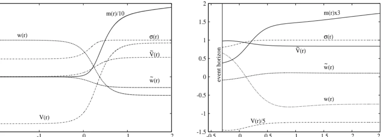
-1 0 1 2 -2 -1 0 1 2 log10(r) σ(r) w~(r) m(r)/10 w(r) V~(r) V(r) -1.5 -1 -0.5 0 0.5 1 1.5 2 -0.5 0 0.5 1 1.5 2 2.5 log10(r) event horizon σ(r) w~(r) m(r)x3 w(r) V~(r) V(r)/5
Figure 1: The profiles of a typical globally regular solution (left) and a black hole solution (right) of the EYMCS equations are presented as a function of the radial coordinater. For these solutions, the mass functionm(r) diverges logarithmically asr→ ∞.
withKbeing an integration constant. One can easily see that the solutions are regular at the origin,r= 0, only ifK= 8κ. The value ofK is not fixeda priorifor black hole solutions.
The asymptotics of the SU(2)×U(1) solutions can easily be read from the general relations (16), (19) and (22). At infinity, the finite mass solutions haveα=±π/2 in (22), with the gauge potentials
V(r) = Φ−8κ∓K 2r2 +O(1/r 4), w(r) = ±1 +w2 r2 +O(1/r 4). (29)
Thus, for the casew(∞) = −1 studied in this work, the parameter q fixing the Abelian electric charge of these solutions isq=−(4κ+K/2) for black holes andq=−8κfor globally regular solutions.
3
Numerical results
We start by noticing that the equations (14) are not affected by the transformation:
r→λr, m→λ2m, ℓ→λℓ, V →V /λ, V˜ →V /λ, α˜ →λα , κ→λκ, (30) whilew,w˜ andσ remain unchanged. It follows that one can always take an arbitrary positive value forα. The usual choice isα= 1, which fixes the EYM length scaleL=p8πG/(3e2), while the mass scale is fixed byM= 8π/(3e2). All other quantities get multiplied with suitable factors ofL. However, in this Section, to avoid cluttering our expressions with a complicated dependence on (G, e), we fix the value ofαatα= 1, and ignore the extra factors ofeandGin the expressions of various global quantities.
Therefore the remaining input parameters are the AdS length scale ℓ and the CS coupling constantκ. Determining the pattern of the solutions in the parameter space represents a very complex task which is outside the scope of this paper. Instead, we analysed in detail a few particular classes of solutions which, hopefully, reflect all relevant properties of the general pattern. For definiteness we setℓ= 1 in our numerical analysis, although we have found nontrivial solutions also for other values of the cosmological constant9.
8
This truncation of the fullSO(6) model shares a number of common features with the five dimensionalN = 4 gauged
SU(2)×U(1) supergravity model considered in [32]. For example, a first integral similar to (28) appears there also. However, the solutions in [32] have an extra dilaton field with a Liouville potential and thus are not asymptotically AdS.
9
In particular, the finite energy solutions survive in the limit Λ→0, being supported by the CS term (this contrasts strongly with the case of a pure EYM theory [12]). A discussion of the asymptotically flat EYMCS solutions will be presented elsewhere.
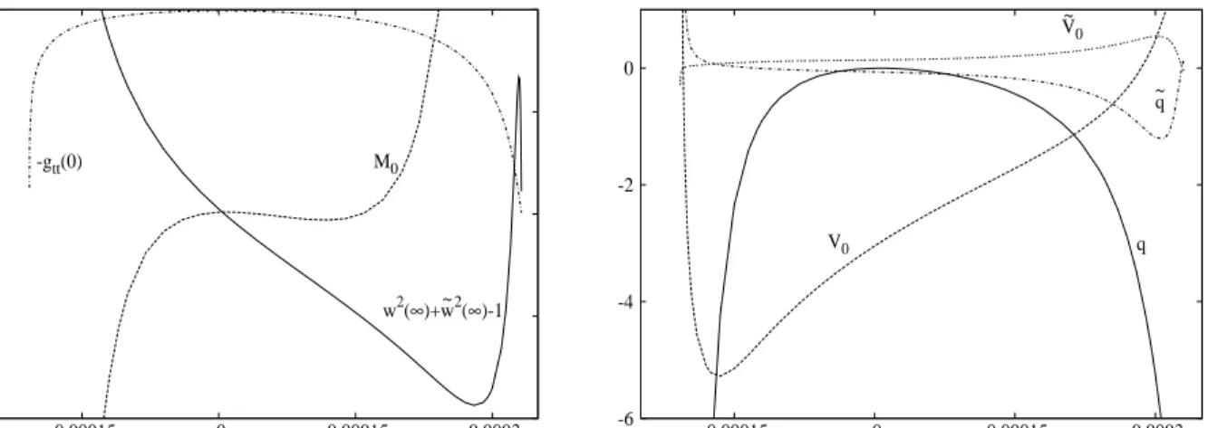
-1 -0.5 0 0.5 1 -0.00015 0 0.00015 0.0003 b -gtt(0) M0 w2(∞)+w~2(∞)-1 -6 -4 -2 0 -0.00015 0 0.00015 0.0003 b V~0 V0 q q ~
Figure 2: A number of relevant parameters are plotted as functions of the coefficientbfor globally regular solutions of the EYMCS model withℓ= 1,κ= 1. These solutions have finite electric charges, which are fixed byq and ˜q.
Instead we have looked for the dependence of the solutions on the value of the CS coefficientκ, which has not been fixeda priori. (This investigation has been partly motivated by the study in [33] of the Einstein-Maxwell-CS system, which revealed a nontrivial dependence of the properties of the solutions on the value ofκ. We shall see that this is also the case for the solutions constructed in this work, which feature a critical value of CS coefficient.)
The resulting set of six ordinary differential equations10 is solved with suitable boundary conditions which result from (16), (17), (19) and (22). The numerics employs a collocation method for boundary-value ordinary differential equations equipped with an adaptive mesh selection procedure [34]. Typical mesh sizes include 103
−104 points. The solutions have a relative accuracy of 10−7. In addition to employing this algorithm, some solutions were also constructed by using a standard Runge-Kutta ordinary differential equation solver. In this approach we evaluate the initial conditions atr= 10−5(orr=r
h+ 10−5), for global
tolerance 10−12, adjusting for shooting parameters and integrating towardsr
→ ∞. We have confirmed that there is good agreement between the results obtained with these two different methods.
The properties of the solutions depend on the input parameters, but it is rather difficult to find a general pattern. However, a feature shared by all asymptotically AdS solutions is that the metric functionsm(r), σ(r) monotonically approach their asymptotic values, which can easily be seen from the corresponding field equations. Also, so far we could not find solutions where the electric potentials V(r), ˜V(r) present oscillations, even though such solutions are allowed.
3.1
The generic solutions
The generic solutions studied here are for thed= 4 + 1 dimensional model, which features a Chern–Simons (CS) term. But solutions with similar properties are found also in the EYM model with no CS term. All these solutions bear a qualitative similarity to those of the more familiard= 3 + 1 EYM model [1], [2]. These solutions can also be seen as higher gauge group generalisations of the EYM solutions in [4], but unlike the latter they feature a nontrivial electric potential, made possible by the larger gauge group. (The electric potential necessarily vanishes for ad= 5 static, spherically symmetricSU(2) gauge field).
Considering first the case of globally regular configurations, one finds that solutions approaching asymp-totically the AdS5 background exist for compact intervals of the initial parametersw′′(0), V(0), V′(0) and σ(0). The values of the parametersw0,w˜0, V0,V˜0,w2,w˜2andqwhich enter the asymptotics of the solutions
10
Although we have solved the second order YM equations in (14), we have also monitored the constraint (15), which was always satisfied with very good accuracy. Also, the equation (15) has been used to construct the asymptotic expansions (16), (17), (19) and (22).
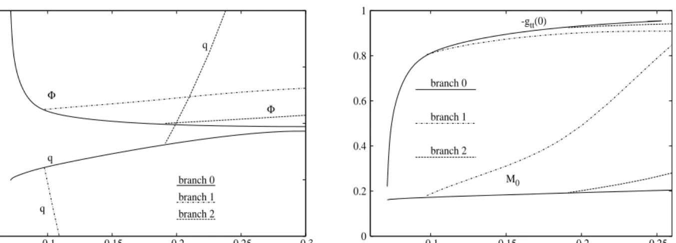
-1 0 1 2 3 0.1 0.15 0.2 0.25 0.3 κ Φ Φ q q q branch 0 branch 1 branch 2 0 0.2 0.4 0.6 0.8 1 0.1 0.15 0.2 0.25 κ -gtt(0) M0 branch 0 branch 1 branch 2
Figure 3: A number of relevant parameters are plotted as functions of the Chern-Simons couplingκfor finite mass, globally regular solutions of the EYMCS model. One can see that new branches of solutions emerge asκincreases.
are fixed by the numerics. (There are also branches of solutions with a different asymptotic behaviour, which stop to exist for finite values ofr. To study these configurations, one needs to employ a metric Ansatz different from (6). Such solutions, being not asymptotically AdS, are of no interest here.)
Of the full set of solutions with AdS asymptotics, we have paid special attention to the physically more interesting case of configurations with a 1/r2decay of the electric potentials at infinity (i.e. V
c= ˜Vc= 0 and
˜
V0w0−V0w˜0 = 0), this being the only case reported in this Section. These solutions have a finite electric charge, although their mass functions will diverge asymptotically since|φ~|=pw2
0+ ˜w206→1 here.
A typical configuration with a regular origin is presented in Figure 1 (left), forκ= 1. One can see that the mass function diverges logarithmically while σ(r), w(r),w(r) and˜ V(r),V˜(r) asymptotically approach some finite values. Solutions with nodes inw(r), ˜w(r) were also found.
In Figure 2 we plot a number of relevant parameters as a function of the coefficientb in the initial data at r = 0 (b = −w′′(0)/2), for a family of asymptotically AdS solutions. (One of the parameters there is M0 appearing in (19), which in Section 5 we argue that it can be taken as the renormalised mass of the solutions; note thatM0 may take also negative values). This branch ends for some finite values ofb, where
−gtt(0) =σ(0)→0 whileV0, q diverge. The condition|φ~×~χ| →0 asr→ ∞has been enforced by treating V(0) as a shooting parameter. Then ˜V′
(0) is a free parameter while σ(0) results from the numerics (the solutions in Figure 2 haveV′
(0)/σ0= 0.15).
The results in Figure 2 show that the for generic solutions w2(∞) + ˜w2(∞)6→1. From (19), this leads to a divergent mass-energy as defined in the usual way. However, one can see that the condition|φ~| →1 is satisfied for a discrete set of the parameterb (e.g. b≃0.3219×10⁻³andb
≃0.6125×10⁻⁵for the data in Figure 2). This suggests the existence of several branches of finite mass solutions parametrised by ˜V′(0) (or, equivalently,V(0)), which is confirmed by the results in the next subsection.
Black hole solutions have been found as well, presenting the same general features. Here also we find a continuum of solutions with arbitrary values of gauge potentials at infinity, the relevant parameters being the values of the gauge potentials at the event horizon as given by (17). Again, finite mass black holes are found only for specific values of the gauge potentials on the horizon.
As a general remark, we note that the presence of the CS term is not crucial for the existence of the generic solutions (i.e.with a divergent mass). We have found solutions with rather similar properties also forκ= 0. Thus, the role of the CS term is indispensable only for the construction ofspecial, finite mass, solutions to be presented in the next subsection.
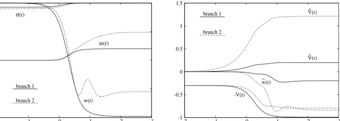
-1 -0.5 0 0.5 1 -2 -1 0 1 2 3 log10(r) branch 1 branch 2 m(r) w(r) σ(r) -1 -0.5 0 0.5 1 1.5 -2 -1 0 1 2 3 log10(r) w~(r) V~(r) V~(r) -V(r) branch 1 branch 2
Figure 4: The profiles of two typical globally regular EYMS solutions are presented as function of the radial coordinater. m(r) andσ(r) are metric functions, whichw(r),w˜(r) andV(r),V˜(r) are non-Abelian potentials.
3.2
Finite mass solutions
3.2.1 Regular configurations
In the numerics, special attention has been paid to solutions with a finite mass. As noted above, in this case, three of the four parameters in the data atr= 0 are fixed. The remaining free parameter was chosen to be V(0) (similar results are found when ˜V(0) is chosen instead).
Remembering the invariance under the parity reflectionφ~→ −φ,~ χ~→ −χ~ it turns out to be sufficient to considerV(0)≥0 (or ˜V(0)≥0).
Thus, corresponding to a choice of the coupling constant κand of the cosmological constant Λ, there exist in principle a family of finite mass charged EYMCS solutions labeled by the value at the origin of one of the electric potentials, in this case,V(0). The pattern of these solutions turns out to be extremely rich, with some unexpected features.
In order to illustrate this, we first fixV(0) = 0.3 and study the solutions as functions of the CS parameter κ. (Qualitatively, the same results have been found when considering other values ofV(0)). The numerical results show that a branch of solutions with ˜w(r) = ˜V(r) = 0 always exists for sufficiently large values ofκ, for instance,κ≥κ0≃0.07 in the present case. These are the solutions of the reducedSU(2)×U(1) model with the asymptotic angle α=π/2. For convenience, we will refer to this branch as themain branch. In the limitκ→κ0 the metric functionσ(r) vanishes at the origin and the solution becomes singular. For all values of the other parameters, no finite mass solutions have been found forκ < κ0.
The interesting feature is that new branches of solutions with notrivial functions ˜w(r), V˜(r) emerge from the main branch at critical values ofκ. In our cases, the first branch of excited solution appearsκ≃0.0953 and a second branch atκ≃0.1875. This behaviour is illustrated in Figure 3, where a number of relavant global parameters are plotted a functions of the CS coupling constantκ. It should be noted that, for a fixed κ, the excited solutions have larger masses than the solutions on themain branch.
The profiles of the two first excited solutions corresponding toκ= 0.2 is presented in Figure 4. One can see that the functionsw,w˜parametrising the magnetic field of the excited solutions develop more pronounced oscillations before becoming constant in the asymptotic region.
It is also natural to study the spectrum of solutions in terms of one of the charges, say ˜q for a fixed value ofκ. The second electric charge q is determined from numerics. The results of our analysis for the valueκ= 0.2 are summarised in Figure 5. In this case, two excited solutions are available. Several relevant parameters are plotted thereversusq˜(see Eqn. (22)) for two excited solutions. Fixing the parity symmetry by means of ˜V′
(0) ≥ 0, the numerical analysis reveals that the solutions of the branch ”1” (respectively ”2”) are characterised by negative (respectively positive) values of ˜q. Also, they exist up to a minimal
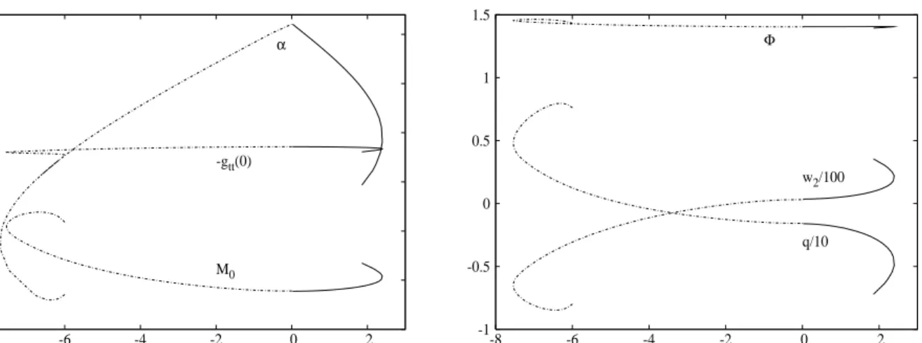
0 0.25 0.5 0.75 1 1.25 1.5 -8 -6 -4 -2 0 2 q ~ -gtt(0) M0 α -1 -0.5 0 0.5 1 1.5 -8 -6 -4 -2 0 2 q ~ q/10 Φ w2/100
Figure 5: A number of relevant parameters are plotted as functions of the electric charge ˜qfor finite mass, globally regular solutions of the EYMCS model with a Chern-Simons coefficientκ= 0.2. The dashed and solid curves denote different branches of solutions.
(respectively maximal) value, say ˜q = ˜qcr. Forκ= 0.2 we have ˜qcr ≈ −7.8 and ˜qcr ≈2.5 respectively, for
the first and second branches. In the limit ˜qcr →0, the excited solutions converge to the main solution. The
ending of the branches at ˜q = ˜qcr is more subtle. Indeed, our numerical results show that another family
of solutions (with larger mass) exists in the region|q˜|<|q˜cr|, backbending from the branch coming directly
from the main solution. These new branches are shown on Figure 5; however, we have not attempted to construct further branches in this region, although they are likely exist.
3.2.2 Black holes
The EYMCS system presents also black hole solutions which were constructed using similar techniques. In contrast with the regular solutions presented above, the main thrust here is confined to the solutions of ourparticular truncationof the full SO(6) model. This restriction is made to simplify an otherwise very complex numerical task.
The Hawking temperature and the entropy of the black holes are given by TH = σ(rh)N′(rh) 4π , S= AH 4G, with AH=V3r 3 h, (31)
whereV3= 2π2is the area ofS3. An interesting feature here is that the finite mass black hole solutions have two free parameters in the event horizon initial data, which were taken to beV(rh) and ˜V(rh). As a result,
and in contrast to the case of globally regular solutions, the two electric chargesqand ˜qare independent for black holes. This leads to a much richer parameter space of solutions.
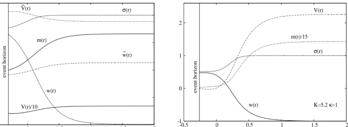
Our numerical results provide evidence for the existence of finite mass black hole solutions of the EYMCS system with a set of four notrivial gauge functions (i.e.for the full groupSO(6)). The profile of a generic black hole corresponding toκ= 0.2 and rh= 0.5 is presented in Figure 6 (left) for ˜q= 0.5, q=−1.5.
However, given the large number of free input parameters, we did not attempt a systematic study of these solutions, concentrating instead on the simpler case of the SU(2)×U(1) truncated model. An interesting feature here is that solutions with AdS asymptotics exist only for the limited interval κmin ≤κ≤κmax of
κ. The limits of this interval depend on the values ofrhand K. Clearly, the range of the electric charge of
these solutions is also bounded. These features are illustrated in Figure 7 (left), for black hole solutions with a fixed horizon radius rh = 1. One can see that asκ →κmin the value at the horizon of metric function
σ(r) tends to zero, as does also the Hawking temperature, while other quantities stay finite. The behaviour of solutions for largeκis less clear, the accuracy decreasing withκ. However, the numerical results seem to
-1 -0.5 0 0.5 1 -0.5 0 0.5 1 1.5 2 event horizon σ(r) w~(r) m(r) w(r) V~(r) V(r)/10 -1 0 1 2 -0.5 0 0.5 1 1.5 2 log10(r) event horizon K=5.2 κ=1 σ(r) m(r)/15 w(r) V(r)
Figure 6: Left: The profiles of a typical non extremal black hole solution of theSO(6) model is presented as a function of the radial coordinater. Right: An extremal black hole solution for ourparticular truncationof the full model.
indicate that this branch ends in a critical solution withσ(rh) close to one and a finite nonzero value ofTH.
Unfortunately, the study of solutions forκ→κmax is a difficult task and the general picture may be much
more complicated. For example, we have noticed the existence there of a secondary branch of solutions, which are close to a finite mass extremal configuration with nontrivial gauge fields. A systematic study of these aspects would require a different parametrisation of the metric line element than (6), and is beyond the scope of this work.
One can also keep κ and K fixed and vary the value of the event horizon radius. As noted above, choosing the values ofκ, K fixes also the electric charge,i.e.,these black holes are in a canonical ensemble. Our numerics indicate that for any K, the value of the gauge field potential at the horizon decreases with rh. For large enough values of the event horizon radius, the solutions become essentially RNAdS black holes,
withw(r) being close to the value−1 everywhere, with the non-Abelian magnetic field vanishing.
However, the picture for small enough values of the horizon radius depends crucially on the value of the integration constant K in the V-equation (29) (i.e.on the Abelian electric charge). Starting with the special value K= 8κ, we plot in Figure 8 a number of relevant features of the solutions, for three different values of the CS coefficientκ. One can see that these non-Abelian black holes behave in a similar way to the vacuum AdS solutions. The small black holes are thermally unstable, the entropy being a decreasing function of the Hawking temperature. They become thermally stable for large enough values of the event horizon radius. In the limit rh → 0, these black holes approach the set of globally regular particle-like
solutions with ˜V(r) = ˜w(r) = 0, discussed above .
The picture is very different when choosing instead K 6= 8κ(see Figure 7 (right)). As an interesting new feature, here an extremal black hole solution is approached for a critical value ofrh. In this case the
horizon is degenerate (i.e.,N(r) has a double root: N(rh) =N′(rh) = 0) and the near horizon geometry is
AdS2×S3.
Asr→rhone finds the approximate form of the solution in the near horizon region:
N(r) =N2(r−rh)2+O(r−rh)3, σ(r) =σh− 3σhw21 2rh (r−rh) +O(r−rh)2, (32) w(r) =wh+w1(r−rh) +O(r−rh)2, V(r) =Vh− σhwh 2κrh (r−rh) +O(r−rh)2, (33)
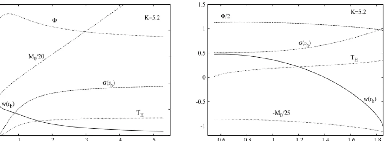
0 0.5 1 1.5 2 2.5 1 2 3 4 5 κ K=5.2 TH M0/20 Φ w(rh) σ(rh) -1 -0.5 0 0.5 1 1.5 0.6 0.8 1 1.2 1.4 1.6 1.8 rh K=5.2 w(rh) Φ/2 TH -M0/25 σ(rh)
Figure 7: The mass parameter M0, the value at the horizon of the metric functionσ(r) and the magnetic gauge potentialw(r), the electrostatic potential Φ and the Hawking temperature are plot as a functions of the CS coupling constantκ(left) and of the event horizon radiusrh(right).
where w1= 32κ2r hℓ2wh(1−w2h) −3α2r2 hℓ2wh2+ 384κ4ℓ2(1−w2h)2−4κ2(24rh4−4rh2ℓ2(wh2−2) + 3α2ℓ2(1−w2h)2) (34) N2= 24r4 h+ 8r2hℓ2−3α2ℓ2(1−w2h)2) 2r4 hℓ2 .
The parametersrh andwh in the above relation are solutions of the equations
32r4 h ℓ2 −12α 2(1 −w2h)2+rh2(16− α2w2 h κ2 ) = 0, (35) 2Kκ+wh(rh2+ 8κ2(w2h−3)) = 0.
Recalling thatK= 2(q−4κ), it follows that all event horizon boundary data (exceptσ(rh)) are fixed by the
κ, ℓand the electric chargeq. (Note the analogy with the extremal Abelian solution case.) This extremal solution differs from the RNAdS one, presenting non-Abelian magnetic hair and a nontrivial metric function σ(r) (see Figure 6 (right)).
As expected, the near horizon structure of the extremal solutions can be extended to a full AdS2×S3 solution of the field equations. This configuration has a line element
ds2= dr 2 1−Λ1r2 6 +r20dΩ23−(1− Λ1r2 6 )dt 2, (36)
and the matter fields
w=w0, V(r) =V0− w0 2κr0
(r−rh). (37)
Forw2
06= 1, this is a non-Abelian solution, with the gauge field living on the three-sphere. The parameters Λ,w0 and the radiusr0 of theS3are constrained by the relation
Λ = 3 r2 0 − πG e2 r2 0w02+ 12κ2(w02−1)2 κ2r4 0 , (38)
the value of the AdS2 cosmological constant Λ1in (36) being Λ1= 6 Λ−r12 0 − πG e2 r2 0w02+ 4κ2(1−w20)2 κ2r4 0 . (39)
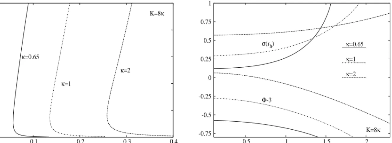
0 8 16 24 32 40 0.1 0.2 0.3 0.4 AH TH K=8κ κ=0.65 κ=1 κ=2 -0.75 -0.5 -0.25 0 0.25 0.5 0.75 1 0.5 1 1.5 2 rh K=8κ κ=0.65 κ=1 κ=2 Φ-3 σ(rh)
Figure 8: The temperature-entropy diagram (left) and the value at the horizon of the metric functionσ(r) and of the electrostatic potential Φ (right) are ploted as functions of the event horizon radiusrh for three different values of the Chern-Simons coupling constantκ. These configurations have an integration constantK= 8κ, and approach the globally regular particle-like solutions asrh→0.
4
Global charges
4.1
The mass and boundary stress tensor
The action and mass of these AdS5 non-Abelian configurations is computed by using a boundary countert-erm prescription. As found in [20], the following countertcountert-erms are sufficient to cancel divergences in five dimensions, for Schwarzschild-AdS black hole solution (in this Section we restore the 8πGand efactors in the expressions): Ict=− 1 8πG Z ∂M d4x√−h " 3 ℓ + ℓ 4R # , (40)
with R the Ricci scalar for the boundary metrich.
(Note also that, as usual, to ensure well-defined Euler-Lagrange field equations, one adds to the action (1), the Gibbons-Hawking surface term [23] Isurf =−8πG1 R∂Md
4x√
−hK, whereKis the trace of the extrinsic curvature for the boundary ∂M.) However, in the presence of matter fields, additional counterterms may be needed to regulate the action [35], which is also the case for the generic non-Abelian solutions discussed in the previous Sections11.
This divergence is cancelled by a supplementary counterterm of the form (with a, bboundary indices): IY M ct =−log( r ℓ) Z ∂M d4x√−h ℓ 2e2 Tr{FabF ab }. (41)
Note that this term is identically zero for the solutions withw2+ ˜w2→1, ˜V w−Vw˜→0.
Using these counterterms and the Gibbons-Hawking boundary term, one can construct a divergence-free boundary stress tensor Tab
Tab= 1 8πG(Kab−Khab− 3 ℓhab+ ℓ 2Eab)− 2ℓ e2log( r ℓ) Tr{FacFbdh cd −14habFcdFcd} , (42) 11
The geometric counterterm (40) regularises also the action of the RNAdS5 black hole solution. However, this does not
hold for anyd= 5 solutions of the Einstein-Maxwell-Λ system. An interesting example here are the AdS black strings with a magneticU(1) field [36], in which case one has to consider an additional matter counterterm on the form (41).
where Eab and K are the Einstein tensor and the trace of the extrinsic curvature Kab for the induced
metric of the boundary, respectively. In this approach, the mass M of the solutions is the conserved charge associated with the Killing vector ∂/∂t[20]. A straightforward computation leads to the following simple result for the mass of the generic EYMCS solutions:
M = 3V3M0
16πG +Mc, with Mc= 3V3ℓ2
64πG . (43)
For the case of black hole solutions of the truncatedSU(2)×U(1) model, we have found that M coincides within the numerical accuracy with the mass computed from the first law of thermodynamics, up to the constant termMc which is usually interpreted as the mass of the pure global AdS5.
From the AdS/CFT correspondence, we expect the non-Abelian hairy black holes to be described by some thermal states in a dual theory formulated in a metric background given by
γabdxadxb=−dt2+ℓ2(dψ2+ sin2ψ(dθ2+ sin2θdϕ2)), (44)
whereψ, θ, ϕare the usual polar angles parametrizingS3.
The matter fields in the dual CFT would interact with a background non-Abelian field, whose expression, as read from (9), (19) is
At =
1
e V˜0[sinψsinθ(Σ16cosϕ+ Σ26sinϕ) + sinψcosθΣ36+ cosψΣ46]−V0Σ56
, Aψ =
1
e (1 +w0) [sinθ(Σ14cosϕ+ Σ24sinϕ) + cosθΣ34]
+ ˜w0[cosψsinθ(Σ15cosϕ+ Σ25sinϕ) + cosψcosθΣ35−sinψΣ45], (45) Aθ =
1
e (1 +w0) sinψ
sinψ(Σ13cosϕ+ Σ23sinϕ)−sinψcosθΣ14cosϕ
+ cosψcosθΣ24sinϕ+ cosψsinθΣ34+ ˜w0sinψ[cosθ(Σ15cosϕ+ Σ25sinϕ)−sinθΣ35], Aϕ =
1
e −(1 +w0) sinψ
sinψsin2θΣ12+ sinψsinθcosθ(Σ13sinϕ−Σ23cosϕ) + cosψsinθ(Σ14sinϕ−Σ24cosϕ)−w˜0sinψsinθ(Σ15sinϕ−Σ25cosϕ), We note that this is still fully anSO(6) gauge field.
The expectation value< τa
b >of the dual CFT stress tensor can be calculated using the relation [37]
√ −γγab< τ bc>= lim r→∞ √ −hhabT bc. (46)
Employing also (42), we find the finite and covariantly conserved stress tensor (withx1=ψ, x2=θ, x3= ϕ, x4=t) 8πG < τa b >= 1 2ℓ M0 ℓ2 + 1 4 1 0 0 0 0 1 0 0 0 0 1 0 0 0 0 −3 − 4πG((w2 0+ ˜w20−1)2+ℓ2( ˜V0w0−V0w˜0)2) e2ℓ3 1 0 0 0 0 1 0 0 0 0 1 0 0 0 0 0 .(47)
Differente.g.from the case of Reissner-Nordstr¨om-AdS Abelian solutions, this stress tensor has a nonvanish-ing trace. Moreover, for the physically relevant case of solutions with a finite electric charge (i.e.|φ~×~χ| →0 asymptotically) one finds that < τa
a >=AY M =−3(w20+ ˜w20−1)2/(2ℓ2e2). This agrees with the general results [38], [39], [35] on the trace anomaly in the presence of an external gauge field, AY M =RF(0)2 , the
coefficientRbeing related to the charges of the fundamental constituent fields in the dual CFT.
4.2
Electric charge(s)
For the solutions with |φ~ ×χ~| → 0 (i.e. ( ˜V0w0−V0w˜0)|r→∞ = 0) the coefficients of the 1/r2 terms in the asymptotic expansion of the electric potentials are finite. Thus, from the Gauss flux theorem one can
formally define the electric charge QE= I ∞ dSk√−gFkt= 4π2 e (qΣ56+ ˜qΣ12), (48)
which is clealy not gauge invariant. (This is a generic problem for the definition of the non-Abelian charges in the absence of a Higgs field, seee.g.[40]).
Perhaps a more proper definition can be given following the reasoning in [41]. In this approach one starts by evaluating the quantity Tr{FitFit},
√
−gTr{FitFit}=√−gTr{DiAtFit}=∂i(√−gTr{AtFit})−√−gTr{AtDiFit}.
Using the Gauss’ law equation, we find that the contribution of the electric field to the total mass then is Ee=− 1 e2 Z dSk√−g ~χ·Dr~χ+ 4V3κ e2 Z dr(|φ~|2 −1)χ~·Drφ g~ tt (49)
Subject to the truncations this expression simplifies; the integral in the second term must be evaluated using the numerical solution, while the surface integral in the first term can be evaluate using only the asymptotic values of the functions.
In the absence of the Chern-Simons term, i.e., whenκ= 0, the contribution of the electric field to the total mass can be written as
Ee=− I ∞ dSk√−gTr{AtFkt} =QEΦ, where Φ=pTr{AtAt}= q V2 0 + ˜V02, QE= 4π2 e V0q+ ˜V0q˜ p V2+ ˜V2, (50)
are the electrostatic potential and the electric charge, respectively. However, one can extend this definition ofΦ and QE to solutions of the EYMCS system. This applies to bothgeneric and specialconfigurations (note thatΦ= Φ,QE= 4π2(sinα q+ cosαq)/e˜ for finite mass solutions).
For finite mass solutions, following [21], one can also define an effective non-Abelian chargeQef f by the
asymptotic behaviour of the metric function N(r), which, to order 1/r4 is similar to that of the RNAdS solution: N(r) = 1 +r 2 ℓ2 − M0 r2 + Q2 ef f r4 +. . . , (51) i.e. Qef f = αp(q2+ ˜q2)ℓ2+ 3(w2 2+ ˜w22)) ℓ . (52)
Concerning a definition of a ”magnetic” flux, the only natural quantity we have at our disposal for this purpose is the Chern–Pontryagin density, which we know is the leading and sole contributing term to the topological charge (”magnetic” flux) of the monopole in 4 + 1 dimensions [42]. There however the gauge group isSO(4) and the model features a iso-four-vector Higgs field.
This quantity can be calculated easily for theSO(6) Ansatz employed in this paper εijklTrFijFkl =−
4! r3(|φ~|
2
−1) Tr Drφ3Σ56+ (Drφε)MΣM4, (53) which vanishes,i.e., the candidate for a magnetic charge for the solutions found in the present work equals zero identically.
5
Further remarks
On general grounds, one expects that extending the known classes of solutions of thed= 5 supergravity to a non-Abelian gauge group would lead to a variety of new physical effects.
This work has been aimed as a first step towards constructing the non-Abelian solutions of the maximal d = 5 gauged supergravity. Restricting to the simplest case of static, spherically symmetric solutions, we have proposed a suitable Ansatz for the gauge fields and presented numerical evidence for the existence of both particle-like and black hole solutions. Our systematic description of the black holes is restricted to a certain truncation of the fullSO(6) model, with the sole purpose of rendering the numerics practicable. In this limited context, we have also found extremal black holes.
As a consequence of the presence of a negative cosmological constant in the model, we have recovered the qualitative properties of the solutions to the usual EYM-Λ model in 3 + 1 dimensions [1], [2]. Notably, some of our solutions to which we have referred asgeneric, are characterised by arbitrary asymptotic values of the potentials parametrising the gauge field. Also, these solutions share another property with those of the 3 + 1 dimensional EYM model, namely that the shooting parameters involved take on a continuum of values. Unlike the latter however, their masses turn out to be divergent in our 4 + 1 dimensional case. This is expected on the basis of the Derrick-type scaling argument. However, we have proposed a regularisation procedure for the mass of these solutions, in the context of the AdS/CFT correspondence. As far as these genericsolutions are concerned, the presence of the Chern–Simons term makes no qualitative difference.
Perhaps the most interesting feature of the EYMCS model is the existence of finite mass solutions. We have referred to these as special solutions and they contrast with the generic ones in that the shooting parameters involved take on a discrete set of values. Thespecialsolutions exist only when the non-Abelian Chern–Simons term is present.
Concerning the physical context of our results, it is in order to make several remarks on the issue of the more general solutions of thed = 5, N = 8 gauged supergravity. This model contains in addition twenty scalars, which are represented by a symmetric unimodular tensor. These scalars have a nontrivial potential approaching a constant negative value at infinity which fixes the value of the effective cosmological constant. No obvious consistent truncation of this sector seems to exist for a gauge groupSO(6) and strictly speaking one should work with the full set of scalars. In principle, at least when this general model is subjected to spherical symmetry, the one dimensional subsystem resulting from the aplication of the Ansatz here can be studied using the same methods as in this paper,i.e., the solutions can be constructed by solving a boundary value problem. One can in that case find the approximate expressions at the origin or event horizon and at infinity. The only obstacle to this task that we see at this moment is the huge complexity of the ensuing equations. Based on the results in this paper, we expect the parameter space of the fullSO(6) solutions of thed= 5, N = 8 model to be very rich. Inclusion of the scalar sector will lead to many new free parameters in the asymptotics and will make any attempt to classify the solutions difficult (involving numerous different ways of approaching a constant negative value at infinity for the scalar potential).
Thegenericnon-Abelian solutions on the other hand will always present a nonvanishing magnetic gauge field on the boundary which appears as a background for the dual theory. (This feature is independent of the presence or absence of scalars.) Thus the expectation value of the dual CFT stress tensor will contain a part which is similar to (47). Configurations with vanishing non-Abelian magnetic field on the boundary, and finite mass, should exist as well, being supported by the CS term. Also, similar to the case of four dimensional EYM non-Abelian solutions in [6], the existence of both spherically symmetric globally regular and hairy black hole solutions with the same set of data at infinity raises the question as to how the dual CFT is able to distinguish between these different bulk configurations.
Concerning future developments of this work, we expect a much richer structure of the non-Abelian so-lutions to be found when relaxing the spacetime symmetries. For example, one may envisage the existence of asymptotically AdS5 solutions which are static and non-spherically symmetric, generalising the configu-rations in [43]. Particularly interesting would be to approach the issue of EYMCS rotating solutions. To our knowledge, the only d >4 rotating solutions with non-Abelian fields known so far in the literature are thed= 5 EYM-SU(2) black holes in [44]. However, the mass of these solutions diverges logarithmically. It is likely that the inclusion of a CS term will lead to finite mass solutions also in that case.
Another very natural direction to be explored is the case of zero cosmological constant, which would be outside the context of N = 8 supergravity but would nonetheless be technically very interesting. For example, this would afford a comparison with the corresponding 3 + 1 dimensional asymptotically flat EYM solutions in [21], which involve only a discrete spectrum of the shooting parameters.
Acknowledgements
One of us (D.H.Tch.) would like to thank Werner Nahm and Ruben Manvelyan for useful discussions. E.R. and D.H.Tch. are pleased to acknowledge enlightening and encouraging discussions with Michael Volkov. This work is carried out in the framework of Science Foundation Ireland (SFI) project RFP07-330PHY. YB is grateful to the Belgian FNRS for financial support. The work of ER was supported by a fellowship from the Alexander von Humboldt Foundation.
References
[1] E. Winstanley, Class. Quant. Grav.16(1999) 1963 [arXiv:gr-qc/9812064].
[2] J. Bjoraker and Y. Hosotani, Phys. Rev. D62(2000) 043513 [arXiv:hep-th/0002098]; J. Bjoraker and Y. Hosotani, Phys. Rev. Lett.84(2000) 1853 [arXiv:gr-qc/9906091].
[3] P. Breitenlohner, D. Maison and G. Lavrelashvili, Class. Quant. Grav.21(2004) 1667 [arXiv:gr-qc/0307029]; O. Sarbach and E. Winstanley, Class. Quant. Grav.18(2001) 2125 [arXiv:gr-qc/0102033].
[4] N. Okuyama and K. i. Maeda, Phys. Rev. D67(2003) 104012 [arXiv:gr-qc/0212022]. [5] E. Radu and D. H. Tchrakian, Phys. Rev. D73(2006) 024006 [arXiv:gr-qc/0508033].
[6] R. B. Mann, E. Radu and D. H. Tchrakian, Phys. Rev. D74(2006) 064015 [arXiv:hep-th/0606004].
[7] J. M. Maldacena, Adv. Theor. Math. Phys. 2 (1998) 231 [Int. J. Theor. Phys. 38 (1999) 1113] [arXiv:hep-th/9711200].
[8] E. Witten, Adv. Theor. Math. Phys.2(1998) 253 [arXiv:hep-th/9802150]. [9] M. Gunaydin, L. J. Romans and N. P. Warner, Nucl. Phys. B272(1986) 598.
[10] M. Cvetic, H. Lu, C. N. Pope, A. Sadrzadeh and T. A. Tran, Nucl. Phys. B 586 (2000) 275 [arXiv:hep-th/0003103].
[11] M. Cvetic, H. Lu and C. N. Pope, arXiv:0908.0131 [hep-th]. [12] M. S. Volkov, Phys. Lett. B524(2002) 369 [arXiv:hep-th/0103038]. [13] E. Radu and D. H. Tchrakian, arXiv:0907.1452 [gr-qc].
[14] Y. Brihaye, A. Chakrabarti and D. H. Tchrakian, Class. Quant. Grav.20(2003) 2765 [arXiv:hep-th/0202141]; Y. Brihaye, A. Chakrabarti, B. Hartmann and D. H. Tchrakian, Phys. Lett. B 561 (2003) 161 [arXiv:hep-th/0212288].
[15] Y. Brihaye, E. Radu and D. H. Tchrakian, Phys. Rev. D75(2007) 024022 [arXiv:gr-qc/0610087]. [16] P. Breitenlohner and D. H. Tchrakian, Class. Quant. Grav.26(2009) 145008 [arXiv:0903.3505 [gr-qc]]. [17] D.H. Tchrakian, Lett. Math. Phys.40(1997) 191-201.
[18] M.B. Green, J.H. Schwarz and E. Witten,Superstring Theory, Cambridge University Press, Cambridge, 1987. [19] J. Polchinski,TASI lectures on D-branes, hep-th/9611050.
[20] V. Balasubramanian and P. Kraus, Commun. Math. Phys.208(1999) 413 [arXiv:hep-th/9902121]. [21] R. Bartnik and J. McKinnon, Phys. Rev. Lett.61(1988) 141.
[22] E. Radu and D. H. Tchrakian, Class. Quant. Grav.22(2005) 879 [arXiv:hep-th/0410154]. [23] G. W. Gibbons and S. W. Hawking, Phys. Rev. D15(1977) 2752.
[24] E. Witten, Phys. Rev. Lett.38(1977) 121.
[25] Y. Brihaye and J. Nuyts, Phys. Lett. B66(1977) 346.
[26] A. H. Chamseddine and M. S. Volkov, Phys. Rev. Lett.79(1997) 3343 [arXiv:hep-th/9707176]; A. H. Chamseddine and M. S. Volkov, Phys. Rev. D57(1998) 6242 [arXiv:hep-th/9711181].
[27] D. Z. Freedman and J. H. Schwarz, Nucl. Phys. B137(1978) 333.
[28] R. Emparan, C. V. Johnson and R. C. Myers, Phys. Rev. D60(1999) 104001 [arXiv:hep-th/9903238]. [29] K. Skenderis, Int. J. Mod. Phys. A16(2001) 740, [arXiv:hep-th/0010138];
M. Henningson and K. Skenderis, JHEP9807(1998) 023 [arXiv:hep-th/9806087]; M. Henningson and K. Skenderis, Fortsch. Phys.48, 125 (2000) [arXiv:hep-th/9812032]. [30] S. Odintsov and S. Nojiri, Int. J. Mod. Phys.A18, 2001 (2003) [arXiv:hep-th/0211023]. [31] T. Hertog and K. Maeda, JHEP0407(2004) 051 [arXiv:hep-th/0404261];
T. Hertog and K. Maeda, Phys. Rev. D71(2005) 024001 [arXiv:hep-th/0409314];
M. Henneaux, C. Martinez, R. Troncoso and J. Zanelli, Phys. Rev. D70(2004) 044034 [arXiv:hep-th/0404236]; J. T. Liu and W. A. Sabra, Phys. Rev. D72(2005) 064021 [arXiv:hep-th/0405171].
[32] A. H. Chamseddine and M. S. Volkov, JHEP0104(2001) 023 [arXiv:hep-th/0101202]. [33] J. Kunz and F. Navarro-Lerida, Mod. Phys. Lett. A21(2006) 2621 [arXiv:hep-th/0610075];
J. Kunz and F. Navarro-Lerida, Phys. Lett. B643(2006) 55 [arXiv:hep-th/0610036]. [34] U. Asher, J. Christiansen and R. D. Russel, Math. Comput. 33 (1979) 659;
U. Asher, J. Christiansen and R. D. Russel, ACM Trans. Math. Softw. 7 (1981) 209. [35] M. M. Taylor-Robinson, arXiv:hep-th/0002125.
[36] A. Bernamonti, M. M. Caldarelli, D. Klemm, R. Olea, C. Sieg and E. Zorzan, JHEP 0801 (2008) 061 [arXiv:0708.2402 [hep-th]].
[37] R. C. Myers, Phys. Rev. D60(1999) 046002.
[38] S. R. Coleman and R. Jackiw, Annals Phys.67(1971) 552; M. S. Chanowitz and J. R. Ellis, Phys. Rev. D7(1973) 2490; S. Deser, M. J. Duff and C. J. Isham, Nucl. Phys. B111(1976) 45.
[39] M. Blau, K. S. Narain and E. Gava, JHEP9909(1999) 018 [arXiv:hep-th/9904179]. [40] M. S. Volkov and D. V. Gal’tsov, Phys. Rept.319(1999) 1 [arXiv:hep-th/9810070]. [41] D. Sudarsky and R. M. Wald, Phys. Rev. D46(1992) 1453.
[42] G. M. O’Brien and D. H. Tchrakian, Mod. Phys. Lett. A4(1989) 1389.
[43] E. Radu, Y. Shnir and D. H. Tchrakian, Phys. Lett. B657(2007) 246 [arXiv:0705.3608 [hep-th]]. [44] Y. Brihaye, E. Radu and D. H. Tchrakian, Phys. Rev. D76(2007) 105005 [arXiv:0707.0552 [hep-th]].