The goal of the course:
provide a comprehensive introduction to the modern study of computer algorithms. The algorithms and data structures selected are basic ones, constituting the background of computer science. The discussions on the theory, design, and implementation of data structures and algorithms, as well as their issues are especially oriented to the applications typical for databases (including very large ones – VLDB), information systems – IS, geographic information systems – GIS, computer graphics, multimedia…
The content of the course:
Algorithms, Abstract Data Types, Computers, Memory
• outline of topic, Euclid algorithm and it’s implication to objects like very big numbers and polynomials, basic data types
• pseudocode (and other conventions)
• abstract data types (stack ADT, queue ADT, list ADT, matrix ADT, the dynamic set ADT)
• models of memory, data in physical memory, data in multimedia systems
Trees and Priority Queues
• trees, binary trees, AVL trees, 2-3-4 trees, red-black trees • heaps, heapsort, priority queues
• B-trees
• data compression and Huffman codes • trees in computer memory
Hashing and Indexing
• hashing and hashing functions • linear chaining, open addressing • extendable hashing
Sorting algorithms
• elementary sorting methods • quicksort
• radix sorting • mergesort • external sorting
Radix searching
• digital search trees • radix search trees
• multiway radix searching • Patricia algorithm
External searching
• indexed sequential access • virtual memory String processing • brute-force algorithm • Knuth-Morris-Pratt algorithm • Boyer-Moore algorithm • Rabin-Karp algorithm Pattern matching • Finite automata
• Longest subsequence problem
Range searching
• Elementary methods • Grid method
• Two-dimensional trees
• Multidimensional range searching
Hierarchical multidimensional data
• quadtrees and octrees • R-trees
Algorithms and Abstract Data Types
Informally, algorithm means is a well-defined computational procedure that takes some value, or set of values, as input and produces some other value, or set of values, as output. An algorithm is thus a sequence of computational steps that transform the input into the output.
Algorithm is also viewed as a tool for solving a well-specified problem, involving computers. The statement of the problem specifies in general terms the desired input/output relationship. The algorithm describes a specific computational procedure for achieving that input/output relationship.
There exist many points of view to algorithms. One if these points is a computational one. A good example of this is a famous Euclid’s algorithm:
for two integers x, y calculate the greatest common divisor gcd (x, y)
Direct implementation of the algorithm looks like:program euclid (input, output);
var x,y: integer;
function gcd (u,v: integer): integer; var t: integer; begin repeat if u<v then begin t := u; u := v; v := t end; u := u-v; until u = 0; gcd := v end; begin
while not eof do begin
readln (x, y);
if (x>0) and (y>0) then writeln (x, y, gcd (x, y)) end;
end.
This algorithm has some exceptional features, nevertheless specific to the computational procedures:
• it is computationally intensive (uses a lot of processor mathematical instructions);
• it has to be changed every time when something of the environment changes, say if numbers are very long and does not fit into a size of variable (numbers like 1000!). (d1) 402387260077093773543702433923003985719374864210↵ 714632543799910429938512398629020592044208486969↵ 404800479988610197196058631666872994808558901323↵ 829669944590997424504087073759918823627727188732↵ 519779505950995276120874975462497043601418278094↵ 646496291056393887437886487337119181045825783647↵ 849977012476632889835955735432513185323958463075↵ 557409114262417474349347553428646576611667797396↵ 668820291207379143853719588249808126867838374559↵ 731746136085379534524221586593201928090878297308↵ 431392844403281231558611036976801357304216168747↵ 609675871348312025478589320767169132448426236131↵ 412508780208000261683151027341827977704784635868↵ 170164365024153691398281264810213092761244896359↵ 928705114964975419909342221566832572080821333186↵ 116811553615836546984046708975602900950537616475↵ 847728421889679646244945160765353408198901385442↵ 487984959953319101723355556602139450399736280750↵ 137837615307127761926849034352625200015888535147↵ 331611702103968175921510907788019393178114194545↵ 257223865541461062892187960223838971476088506276↵ 862967146674697562911234082439208160153780889893↵ 964518263243671616762179168909779911903754031274↵ 622289988005195444414282012187361745992642956581↵ 746628302955570299024324153181617210465832036786↵ 906117260158783520751516284225540265170483304226↵ 143974286933061690897968482590125458327168226458↵ 066526769958652682272807075781391858178889652208↵ 164348344825993266043367660176999612831860788386↵ 150279465955131156552036093988180612138558600301↵ 435694527224206344631797460594682573103790084024↵ 432438465657245014402821885252470935190620929023↵ 136493273497565513958720559654228749774011413346↵ 962715422845862377387538230483865688976461927383↵ 814900140767310446640259899490222221765904339901↵ 886018566526485061799702356193897017860040811889↵ 729918311021171229845901641921068884387121855646↵ 124960798722908519296819372388642614839657382291↵ 123125024186649353143970137428531926649875337218↵ 940694281434118520158014123344828015051399694290↵ 153483077644569099073152433278288269864602789864↵ 321139083506217095002597389863554277196742822248↵ 757586765752344220207573630569498825087968928162↵ 753848863396909959826280956121450994871701244516↵ 461260379029309120889086942028510640182154399457↵ 156805941872748998094254742173582401063677404595↵ 741785160829230135358081840096996372524230560855↵ 903700624271243416909004153690105933983835777939↵ 410970027753472000000000000000000000000000000000↵ 000000000000000000000000000000000000000000000000↵ 000000000000000000000000000000000000000000000000↵ 000000000000000000000000000000000000000000000000↵ 000000000000000000000000000000000000000000000000↵ 000000000000000000000000
For algorithms of applications in the focus of this course, like databases, information systems, etc., they are usually understood in a slightly different way, more like tools to achieve input/output relationship. The example of an algorithm in such sense would be a sorting procedure. This procedure is frequently appearing in a transaction (a prime operation in information systems or databases), and even while the same transaction, the sorting:
• is repeated many times; • in a various circumstancies; • with different types of data.
Pseudocode
The notation language to describe algorithms is needed. This language called
pseudocode, often is a lingua franca.
Pseudocode is used to express algorithms in a manner that is independent of a particular programming language. The prefix pseudo is used to emphasize that this code is not meant to be compiled and executed on a computer. The reason for using pseudocode is that it allows one to convey basic ideas about an algorithm in general terms. Once programmers understand the algorithm being expressed by pseudocode, they can implement the algorithm in the programming language of their choice. This, in essence, is the difference between pseudocode and a computer program. A pseudocode program simply states the steps necessary to perform some computation, while the corresponding computer program is the translation of these steps into the syntax of a particular programming language.
Kind of mixed sentences, expressions, etc. derived from Pascal, from C, and from JAVA (sometimes) will be used to express algorithms. There will be no worry about how the algorithm will be implemented. This ability to ignore implementation details when using pseudocode will facilitate analysis by allowing us to focus solely on the computational or behavioural aspects of an algorithm. Constructs of pseudocode:
•
assignments;
•
for … to … [step] … do [in steps of];
•
while … do;
•
do … while;
•
begin … end;
•
if … then … else;
•
pointer, and null pointer;
•
arrays;
•
composite data types;
•
procedure and its name;
Abstract Data Types
A theoretical description of an algorithm, if realized in application is affected very much by:
• computer resources, • implementation, • data.
To avoid unnecessary troubles, limitations, specificity, etc. in the design of algorithm, some additional theory has to be used.
Such a theory include fundamental concepts (guidelining the content of the course): • concepts of Abstract Data Type (ADT) or data type, or data structures;
• tools to express operations of algorithms;
• computational resources to implement the algorithm and test its functionality; • evaluation of the complexity of algorithms.
Level of Abstraction
The level of abstraction is one of the most crucial issues in the design of algorithms. The term abstraction refers to the intellectual capability of considering an entity apart from any specific instance of that entity. This involves an abstract or logical description of components:
• the data required by the software system,
• the operations that can be performed on this data.
The use of data abstraction during software development allows the software designer to concentrate on how the data in the system is used to solve the problem at hand, without having to be concerned with how the data is represented and manipulated in computer memory.
Abstract Data Types
The development of computer programs is simplified by using abstract representations of data types (i.e., representations that are devoid of any implementation considerations), especially during the design phase.
Alternatively, utilizing concrete representations of data types (i.e., representations that specify the physical storage of the data in computer memory) during design introduces:
• unnecessary complications in programming (to deal with all of the issues involved in implementing a data type in the software development process), • a yield a program that is dependent upon a particular data type implementation.
An abstract data type (ADT) is defined as a mathematical model of the data objects that make up a data type, as well as the functions that operate on these objects (and sometime impose logical or other relations between objects).
So ADT consist of two parts: data objects and operations with data objects. The operations that manipulate data objects are included in the specification of an ADT. At this point it is useful to distinguish between ADTs, data types, and data structures.
The term data type refers to the implementation of the mathematical model specified by an ADT. That is, a data type is a computer representation of an ADT. The term data structure refers to a collection of computer variables that are connected in some specific manner. This course is concerned also with using data structures to implement various data types in the most efficient manner possible. The notion of data type include built-in data types. Built-in data types are related to a programming language.
A programming language typically provides a number of built-in data types. For example, the integer data type in Pascal, or int data type available in the C programming language provide an implementation of the mathematical concept of an integer number.
Consider INTEGER ADT, which:
• defines the set of objects as numbers (−infinity, … -2, -1, 0, 1, 2, ..., +infinity); • specifies the set of operations: integer addition, integer subtraction, integer
multiplication, div (divisor), mod (remainder of the divisor), logical operations like <, >, =, etc.
The specification of the INTEGER ADT does not include any indication of how the data type should be implemented. For example, it is impossible to represent the full range of integer numbers in computer memory; however, the range of numbers that will be represented must be determined in the data type implementation.
Built-in data type INT in C, or INTEGER in Pascal are dealing with the set of objects as numbers in the range (minint, … -2, -1, 0, 1, 2, …, maxint), and format of these numbers in computer memory can vary between one's complement, two's complement, sign-magnitude, binary coded decimal (BCD), or some other format. The implementation of an INTEGER ADT involves a translation of the ADT's specifications into the syntax of a particular programming language. This translation consists of the appropriate variable declarations necessary to define the data
elements, and a procedure or accessing routine that implements each of the operations required by the ADT.
The INTEGER ADT when implemented according to specification gives a freedom to programmers. Generally they do not have to concern themselves with these implementation considerations when they use the data type in a program.
In many cases the design of a computer program will call for data types that are not available in the programming language used to implement the program. In these cases, programmers must be able to construct the necessary data types by using built-in data types. This will often involve the construction of quite complicated data structures. The data types constructed in this manner are called user-defined data types.
The design and implementation of data types as well as ADTs are often focused on
user-defined data types. Then a new data type has to be considered from two different viewpoints:
• a logical view;
• an implementation view.
The logical view of a data type should be used during program design. This is simply the model provided by the ADT specification.
The implementation view of a data type considers the manner in which the data elements are represented in memory, and how the accessing functions are implemented. Mainly it is to be concerned with how alternative data structures and accessing routine implementations affect the efficiency of the operations performed by the data type.
There should be only one logical view of a data type, however, there may be many
different approaches to implementing it.
Taking the whole proccess of ADT modeling and implementation into account, many different features have to be considered. One of these characteristics is is an interaction between various ADTs, data types, etc. In this course a so-called
covering ADT will be used to model the behaviour of a specific ADT and to implement it.
The STACK ADT
This ADT covers a set of objects as well as operations performed on these objects: • Initialize (S) – creates a necessary structured space in computer memory to
locate objects in S;
• Pop – deletes object from the stack that was most recently inserted into; • Top – returns an object from the stack that was most recently inserted into; • Kill (S) - releases an amount of memory occupied by S.
The operations with stack objects obey LIFO property: Last-In-First-Out. This is a logical constrain or logical condition.
The operations Initialize and Kill are more oriented to an implementation of this ADT, but they are important in some algorithms and applications too.
The stack is a dynamic data set with a limited access to objects. The model of application to illustrate usage of a stack is:
calculate the value of an algebraic expression.
If the algebraic expression is like:9*(((5+8)+(8*7))+3)
then the sequence of operations of stack to calculate the value would be:
push(9); push(5); push(8); push(pop+pop); push(8); push(7); push(pop*pop); push(pop+pop); push(3); push(pop+pop); push(pop*pop); writeln(pop).
The content of stack after each operation will be:
7
8 8 8 56 3 5 5 13 13 13 13 69 69 72
9 9 9 9 9 9 9 9 9 9 648 nil
The stack is useful also to verify the correctness of parentheses in an algebraic expression.
If objects of stack fit to ordinary variables the straightforward implementation will look like expressed below.
type link=^node;
node=record key:integer; next:link; end; var head,z:link; procedure stackinit; begin new(head); new(z); head^.next:=z; z^.next:=z end;
procedure push(v:integer); var t:link; begin new(t); t^.key:=v; t^.next:=head^.next; head^.next:=t end;
function pop:integer; var t:link; begin t:=head^.next; pop:=t^.key; head^.next:=t^.next; dispose(t) end;
function stackempty:boolean;
begin stackempty:=(head^.next=z) end.
Implementation by the built-in data type of array: const maxP=100;
var stack: array[0..maxP]of integer; p:integer; procedure push(v:integer);
begin stack[p]:=v; p:=p+1 end; function pop:integer;
begin p:=p-1; pop:=stack[p] end; procedure stackinit;
begin p:=0 end;
function stackempty:boolean;
begin stackempty:=(p=<0) end.
The algebraic expression is implemented by using stack:
stackinit; repeat
if c=')' then write(chr(pop)); if c='+' then push(ord(c)); if c='*' then push(ord(c)); while (c=>'0') and (c=<'9') do
begin write(c); read(c) end; if c<>'(' then write('');
until eoln;
The QUEUE ADT
This ADT covers a set of objects as well as operations performed on objects:
• queueinit (Q) – creates a necessary structured space in computer memory to locate objects in Q;
• put (x) – inserts x into Q;
• get – deletes object from the queue that has been residing in Q the longest; • head – returns an object from the queue that has been residing in Q the longest; • kill (Q) – releases an amount of memory occupied by Q.
The operations with queue obey FIFO property: First-In-First-Out. This is a logical constrain or logical condition. The queue is a dynamic data set with a limited access to objects. The application to illustrate usage of a queue is:
queueing system simulation (system with waiting lines)
(implemented by using the built-in type of pointer) type link=^node;node=record key:integer; next:link; end; var head,tail,z:link;
procedure queueinit; begin
new(head); new(z);
head^.next:=z; tail^.next=z; z^.next:=z end;
procedure put(v:integer); var t:link; begin new(t); t^.key:=v; t^.next:=tail^.next; tail^.next:=t end;
function get:integer; var t:link;
begin
t:=head^.next; get:=t^.key;
head^.next:=t^.next; dispose(t)
end;
function queueempty:boolean;
begin queueempty:=(head^.next=z;tail^.next=z) end. The queue operations by array:
const max=100;
var queue:array[0..max] of integer; head,tail:integer;
procedure put(v:integer); begin
queue[tail]:=v; tail:=tail+1; if tail>max then tail:=0 end;
function get: integer;
begin get:=queue[head]; head:=head+1; if head>max then head:=0
end;
procedure queueinitialize; begin head:=0; tail:=0 end; function queueempty:boolean;
begin queueempty:=(head=tail) end.
The Queue Implementation
A queue is used in computing in much the same way as it is used in everyday life: • to allow a sequence of items to be processed on a first-come-first-served basis. In most computer installations, for example, one printer is connected to several different machines, so that more than one user can submit printing jobs to the same printer. Since printing a job takes much longer than the process of actually transmitting the data from the computer to the printer, a queue of jobs is formed so that the jobs print out in the same order in which they were received by the printer. This has the irritating consequence that if your job consists of printing only a single page while the job in front of you is printing an entire 200-page thesis, you must still wait for the large job to finish before you can get your page.
(All of which illustrates that Murphy's law applies equally well to the computer world as to the 'real' world, where, when you wish to buy one bottle of ketchup in a supermarket, you are stuck behind someone with a trolley containing enough to stock the average house for a month.)
From the point of view of data structures, a queue is similar to a stack, in that data are stored in a linear fashion, and access to the data is allowed only at the ends of the queue. The actions allowed on a queue are:
• Creating an empty queue.
• Testing if a queue is empty.
• Adding data to the tail of the queue.
• Removing data from the head of the queue.
These operations are similar to those for a stack, except that pushing has been replaced by adding an item to the tail of the queue, and popping has been replaced by removing an item from the head of the queue. Because queues process data in the same order in which they are received, a queue is said to be a first-in-first out or
FIFO data structure.
Just as with stacks, queues can be implemented using arrays or lists. For the first of all, let’s consider the implementation using arrays.
Define an array for storing the queue elements, and two markers: • one pointing to the location of the head of the queue,
• the other to the first empty space following the tail.
When an item is to be added to the queue, a test to see if the tail marker points to a valid location is made, then the item is added to the queue and the tail marker is incremented by 1. When an item is to be removed from the queue, a test is made to see if the queue is empty and, if not, the item at the location pointed to by the head marker is retrieved and the head marker is incremented by 1.
This procedure works well until the first time when the tail marker reaches the end of the array. If some removals have occurred during this time, there will be empty space at the beginning of the array. However, because the tail marker points to the end of the array, the queue is thought to be 'full' and no more data can be added. We could shift the data so that the head of the queue returns to the beginning of the
array each time this happens, but shifting data is costly in terms of computer time, especially if the data being stored in the array consist of large data objects.
A more efficient way of storing a queue in an array is to “wrap around” the end of the array so that it joins the front of the array. Such a cfrcular array allows the entire
array (well, almost, as we'll see in a bit) to be used for storing queue elements without ever requiring any data to be shifted. A circular array with QSIZE elements (numbered from 0 to QSIZE-1) may be visualized:
The array is, of course, stored in the normal way in memory, as a linear block of QSIZE elements. The circular diagram is just a convenient way of representing the data structure.
We will need Head and Tail markers to indicate the location of the head and the location just after the tail where the next item should be added to the queue, respectively. An empty queue is denoted by the condition Head = Tail:
At this point, the first item of data would be added at the location indicated by the Tail marker, that is, at array index 0. Adding this element gives us the situation:
Let us use the queue until the Tail marker reaches QSIZE-1. We will assume that some items have been removed from the queue, so that Head has moved along as well:
Now we add another element to the queue at the location marked by Tail, that is, at array index QSIZE-1. The Tail marker now advances one step, which positions it at array index 0. The Tail marker has wrapped around the array and come back to its starting point. Since the Head marker has moved along, those elements at the beginning of the array from index 0 up to index Head-1 are available for storage.
Using a circular array means that we can make use of these elements without having to shift any data.
In a similar way, if we keep removing items from the queue, eventually Head will point to array index QSIZE-1. If we remove another element, Head will advance another step and wrap around the array, returning to index 0.
We have seen that the condition for an empty queue is that Head == Tail. What is the condition for a full queue? If we try to make use of all the array elements, then in a full queue, the tail of the queue must be the element immediately prior to the head. Since we are using the Tail marker to point to the array element immediately following the tail element in the queue, Tail would have to point to the same location as Head for a full queue. But we have just seen that the condition Head == Tail is the condition for an empty queue. Therefore, if we try to make use of all the array elements, the conditions for full and empty queues become identical. We therefore impose the rule that we must always keep at least one free space in the array, and that a queue becomes full when the Tail marker points to the location immediately prior to Head.
We may now formalize the algorithms for dealing with queues in a circular array. • Creating an empty queue: Set Head = Tail = 0.
• Testing if a queue is empty: is Head == Tail?
• Testing if a queue is full: is (Tail + 1) mod QSIZE == Head?
• Adding an item to a queue: if queue is not full, add item at location Tail and set Tail = (Tail + 1) mod QSIZE.
• Removing an item from a queue: if queue is not empty, remove item from location Head and set Head = (Head + 1) mod QSIZE.
The mod operator ensures that Head and Tail wrap around the end of the array properly.
For example, suppose that Tail is QSIZE-1 and we wish to add an item to the queue. We add the item at location Tail (assuming that the queue is not full) and then Set Tail
((QSIZE - 1) + 1) mod QSIZE = QSIZE mod QSIZE = 0 The List ADT
A list is one of the most fundamental data structures used to store a collection of data items.
The importance of the List ADT is that it can be used to implement a wide variety of other ADTs. That is, the LIST ADT often serves as a basic building block in the construction of more complicated ADTs.
A list may be defined as a dynamic ordered n-tuple:
L == (l1, 12, ….., ln)
The use of the term dynamic in this definition is meant to emphasize that the elements in this n-tuple may change over time.
Notice that these elements have a linear order that is based upon their position in the list.
The first element in the list, 11, is called the headof the list.
The last element, ln, is referred to as the tail of the list.
The number of elements in a list L is refered to as the length of the list. Thus the empty list, represented by (), has length 0.
A list can homogeneous or heterogeneous.
In many applications it is also useful to work with lists of lists. In this case, each element of the list is itself a list. For example, consider the list
((3), (4, 2, 5), (12, (8, 4)), ())
The operations we will define for accessing list elements are given below. For each of these operations, L represents a specific list. It is also assumed that a list has a current position variable that refers to some element in the list. This variable can be used to iterate through the elements of a list.
0.Initialize ( L ). This operation is needed to allocate the amount of memory and to give a structure to this amount.
1. Insert (L, x, i). If this operation is successful, the boolean value true is returned; otherwise, the boolean value false is returned.
2. Append (L, x). Adds element x to the tail of L, causing the length of the list to become n+1. If this operation is successful, the boolean value true is returned; otherwise, the boolean value false is returned.
3. Retrieve (L, i). Returns the element stored at position i of L, or the null value if position i does not exist.
4. Delete (L, i). Deletes the element stored at position i of L, causing elements to move in their positions.
5. Length (L). Returns the length of L.
6. Reset (L). Resets the current position in L to the head (i.e., to position 1) and returns the value 1. If the list is,empty, the value 0 is returned.
7. Current (L). Returns the current position in L.
8. Next (L). Increments and returns the current position in L.
Note that only the Insert, Delete, Reset, and Next operations modify the lists to which they are applied. The remaining operations simply query lists in order to obtain information about them.
Sequential Mapping
If all of the elements that comprise a given data structure are stored one after the other in consecutive memory locations, we say that the data structure is sequentially mappedinto computer memory.
Sequential mapping makes it possible to access any element in the data structure in constant time. Given the starting address of the data structure in memory, we can find the address of any element in the data structure by simply calculating its offset from the starting address.
An array is an example of a sequentially mapped data structure:
Because it takes the same amount of time to access any element, a sequentially-mapped data structure is also called a random access data structure.
That is, the accessing time is independent of the size of the data structure, and therefore requires O(l) time.
List Operations Insert and Delete with Single-linked List and Double-linked List:
The Skip Lists:
The abstract data type MATRIX is used to represent matrices, as well as the operations defined on matrices. A matrix is defined as a rectangular array of elements arranged by rows and columns. A matrix with n rows and m columns is said to have row dimension n, column dimension m, and order n x m. An element of a matrix M is denoted by ai,j. representing the element at row i and column j.
The example of matrix:
Numerous operations are defined on matrices. A few of these are:
1. InitializeMatrix (M) – creates a necessary structured space in computer memory to locate matrix.
2. RetrieveElement (i, j, M) – returns the element at row i and column j of matrix
M.
3. AssignElement (i, j, x, M) – assigns the value x to the element at row i and column j of matrix M.
4. Assignment (MI, M2) – assigns the elements of matrix M1 to those of matrix M2. Logical condition: matrices M1and M2 must have the same order.
5. Addition (MI, M2) – returns the matrix that results when matrix M1 is added to matrix M2. Logical condition: matrices M1 and M2must have the same order. 6. Negation (M) –returns the matrix that results when matrix M is negated.
7. Subtraction (MI, M2) – returns the matrix that results when matrix M1 is subtracted from matrix M2. Logical condition: matrices M1 and M2must have the same order.
8. Scalar Multiplication (s, M) – returns the matrix that results when matrix M is multiplied by scalar s.
9. Multiplication (MI, M2) – returns the matrix that results when matrix M1 is multiplied by matrix M2. The column dimension of M1 must be the same as the row dimension of M2. The resultant matrix has the same row dimension as M1, the same column dimension as M2.
10.Transpose(M) – returns the transpose of matrix M. 11.Determinant(M) – returns the determinant of matrix M.
12.Inverse(M) – returns the inverse of matrix M.
13.Kill (M) – releases an amount of memory occupied by M.
Many programming languages have this data type implemented as built-in one, but usually in some restricted way. Nevertheless an implementation of this ADT must provide a means for representing matrix elements, and for implementing the operations described above. It is highly desirable to treat elements of the matrix in a
uniform way, paying no attention whether elements are numbers, long numbers, polynomials, other types of data.
The DYNAMIC SET ADT The set is a fundamental structure in mathematics. Compuer science view to a set:
• it groups objects together;
• the objects in a set are called the elements or members of the set;
• these elements are taken from the universal set U, which contains all possible set elements;
• all the members of- a given set are unique.
The number of elements contained in a set S is referred to as the cardinality of S, denoted by |S|. It is often refered to a set with cardinality n as an n-set.
The elements of a set are not ordered. Thus, {1, 2, 3} and {3, 2, 1} represent the same set.
Mathematical operations with sets:
• an element x is (or is not) a member of the set S; • the empty set;
• two sets A and B are equal (or not);
• an A is said to be a subset of B (the empty set is a subset of every set); • the union of A and B;
• the intersection of A and B; • the difference of A and B;
In computer science it is often useful to consider set-like structures in which the ordering of the elements is important, such sets will be refered as an ordered n-tuple, like (al, a2, … an).
The concept of a set serves as the basis for a wide variety of useful abstract data types. A large number of computer applications involve the manipulation of sets of data elements. Thus, it makes sense to investigate data structures and algorithms that support efficient implementation of various operations on sets.
Another important difference between the mathematical concept of a set and the sets considered in computer science:
• a set in mathematics is unchanging, while the sets in CS are considered to change over time as data elements are added or deleted.
Thus, sets are refered here as dynamic sets. In addition, we will assume that each element in a dynamic set contains an identifying field called a key, and that a total ordering relationship exists on these keys.
It will be assumed that no two elements of a dynamic set contain the same key. The concept of a dynamic set as an DYNAMIC SET ADT is to be specified, that is, as a collection of data elements, along with the legal operations defined on these data elements.
If the DYNAMIC SFT ADT is implemented properly, application programmers will be able to use dynamic sets without having to understand their implementation details. The use of ADTs in this manner simplifies design and development, and promotes reusability of software components.
A list of general operations for the DYNAMIC SET ADT. In each of these operations, S represents a specific dynamic set:
1. Search(S, k). Returns the element with key k in S, or the null value if an element with key k is not in S.
2. Insert(S, x). Adds element x to S. If this operation is successful, the boolean value true is returned; otherwise, the boolean value false is returned.
3. Delete(S, k). Removes the element with key k in S. If this operation is successful, the boolean value true is returned; otherwise, the boolean value false
is returned.
4. Minimum(S). Returns the element in dynamic set S that has the smallest key value, or the null value if S is empty.
5. Maximum(S). Returns the element in S that has the largest key value, or the null
value if S is empty.
6. Predecessor(S, k). Returns the element in S that has the largest key value less than k, or the null value if no such element exists.
7. Successor(S, k). Returns the element in S that has the smallest key value greater than k, or the null value if no such element exists.
In addition, when considering the DYNAMIC SET ADT (or any modifications of this ADT) we will assume the following operations are available:
1. Empty(S). Returns a boolean value, with true indicating that S is an empty dynamic set, and false indicating that S is not.
2. MakeEmpty(S). Clears S of all elements, causing S to become an empty dynamic set.
Since these last two operations are often trivial to implement, they generally are to be omitted.
In many instances an application will only require the use of a few DYNAMIC SET
operations. Some groups of these operations are used so frequently that they are given special names:
the ADT that supports Search, Insert, and Delete operations is called the
DICTIONARY ADT;
the STACK, QUEUE, and PRIORITY QUEUE ADTs are all special types of dynamic sets.
A variety of data structures will be described in forthcoming considerations that they can be used to implement either the DYNAMIC SET ADT, or ADTs that support specific subsets of the DYNAMIC SET ADT operations.
Each of the data structures described will be analyzed in order to determine how efficiently they support the implementation of these operations. In each case, the analysis will be performed in terms of n, the number of data elements stored in the dynamic set.
This analysis will demonstrate that there is no optimal data structure for implementing dynamic sets.
Rather, the best implementation choice will depend upon: • which operations need to be supported,
• the frequency with which specific operations are used, • and possibly many other factors.
As always, the more we know about how a specific application will use data, the better we can fine tune the associated data structures so that this data can be accessed efficiently.
Data are organized in computer memory. According to the applications of interest, three types of memory can be considered:
• Primary (RAM) • Secondary (HDD)
• Ternary (CD-ROM, Video-tape, magnetic tape like streamer, etc.) Primary memory
It is a homogeneous one, the accessible amount of memory is a smallest one (byte) and the access time to any of the elements of memory is constant O(1), it is measured in nano-seconds:
While working with data structures, however, primary memory is managed in a
complicated way too. First, let us make a distinction between static and dynamic
data structures.
A data structure is said to be static if a fixed amount of memory is allocated for that data structure before program execution (i.e., at compile time). That is, the amount of memory allocated to a static data structure does not change during program execution.
A dynamic data structure requires to allocate an amount of memory as it is needed
during program execution-this is referred to as dynamic memory allocation. Thus, with a dynamic data structure, the amount of memory that can be used by the data structure is not fixed at compile time.
It is useful to view this model as a one-dimensional array of storage locations (or bytes) that is divided into three parts. Variables that will persist in memory throughout the execution of the program are allocated in static memory. The amount of storage allocated to static memory is determined at compile time, and this amount does not change during program execution.
A run-time stack is maintained by the computer system in low memory. The amount of storage that the run-time stack uses will vary during program execution. The arrows emanating from the run-time stack indicate that the runtime stack "grows" toward high memory and "shrinks" toward low memory. Each time a procedure is called in a program, an activation record is created and stored in computer memory on the run-time stack.
This activation record contains storage for all variables declared in the procedure, as well as either a copy of, or a reference to, the parameters that are being passed to the procedure. In addition, an activation record must contain some information that specifies where program execution will resume when the procedure is completed. At the completion of the procedure, the associated activation record will be removed from the run-time stack, and program control will return to the point specified in the activation record.
Finally, the logical model shows a free store that "grows" toward low memory and "shrinks" toward high memory. Memory that is allocated at run time (i.e., dynamically) is stored on the free store.
Note that the run-time stack and the free store "grow" toward each other in this model. Thus, an obvious error situation occurs if either too much memory is dynamically allocated without reclaiming it, or too many activation records are created.
While memory allocation and deallocation on the run-time stack are controlled by the computer system itself, such may not be the case for the free store.
In many programming languages, the responsibility of reclaiming dynamically allocated memory is the programmer's. If the memory is not reclaimed by the programmer, then it will remain on the free store.
This approach to reclaiming dynamically allocated memory is referred to as the
explicit approach. On the other hand, in an implicit approach to the deallocation of dynamic memory, memory management functions provided by the system are responsible for reclaiming memory as it is no longer needed. The implicit approach is usually called garbage collection.
Secondary memory
This memory also is referred to as a disc-memory (HDD). It consist of units of equal size (so-called pages, or clusters). Data to be stored in this memory has to be organized into files. Clusters ar much bigger in size comparing to bytes. Usually a few clusters are allocated to one file.
Also there is an index stored in a specific cluster (as for disc-memory, it’s so-called zero-track) and having all files on that disc listed. The read operation (as well as write one) is dealing with clusters, and transfer the whole information of cluster to the main memory.
index cluster
record, specifying a location of a file
clusters allocated to a specific file
Furthermore, the access time for main memory is typically orders of magnitude faster than the access time for secondary storage. For this reason, it is preferable to implement data structures in main memory- refered to these as internal data structures.
In general, secondary storage will be used only if a data structure is too large to fit in main memory. Data structures that reside in secondary storage are refered to as
external data structures.
Ternary memory
This name refers to magnetic tapes, CD-ROMs, video-tapes, etc.: specifications of such memory are – the access time could last even 1 minute, the clusters are huge, they are of different size, etc…
External Memory Algorithms
Data sets in large applications are often too massive to fit completely inside the computer's internal memory. The resulting input/output communication (or I/O) between fast internal memory and slower external memory (such as disks) can be a major performance bottleneck.
The design and analysis of external memory algorithms (also known as EM algorithms or out-of-core algorithms or I/O algorithms). External memory algorithms are often designed using the parallel disk model (PDM). The three machine-independent measures of an algorithm's performance in PDM are:
• the number of I/O operations performed, • the CPU time,
• the amount of disk space used.
PDM allows for multiple disks (or disk arrays) and parallel CPUs, and it can be generalized to handle cache hierarchies, hierarchical memory, and tertiary storage. Experiments on some newly developed algorithms for spatial databases incorporating these paradigms, implemented using TPIE (Transparent Parallel I/O programming Environment), show significant speedups over currently used methods.
For reasons of economy, general-purpose computer systems usually contain a hierarchy of memory levels, each level with its own cost and performance characteristics. At the smallest scale, CPU registers and caches are built with the fastest but most expensive memory. For internal main memory, dynamic random access memory (DRAM) is typical. At a larger scale, inexpensive but slower magnetic disks are used for external mass storage, and even slower but larger-capacity devices such as tapes and optical disks are used for archival storage.
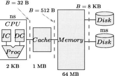
Figure depicts an example of memory hierarchy and its characteristics. The memory hierarchy of a uniprocessor, consisting of registers, data cache, level 2 cache, internal memory, and disk. The B parameter denotes the block transfer size between two adjacent levels of the hierarchy. The size of each memory level is indicated at the bottom.
Most modern programming languages are based upon a programming model in which memory consists of one uniform address space. The notion of virtual memory allows the address space to be far larger than what can fit in the internal memory of
the computer. A natural tendency for programmers is to assume that all memory references require the same access time. In many cases, such an assumption is reasonable (or at least doesn't do any harm), especially when the datasets are not large. The utility and elegance of this programming model are to a large extent the reason why it has flourished in the software industry.
However, not all memory references are created equal. Large address spaces span multiple levels of memory hierarchy, and accessing the data in the lowest levels of memory is orders of magnitude faster than accessing the data at the higher levels. For example, loading a register takes on the order of a nanosecond (10-9 seconds) whereas the latencyof accessing data from a disk is several miliseconds (10-3 seconds). The relative difference in access time is more than a million. The Input/Output communication (or simply I/O) between levels of memory is often the bottleneck in applications that process massive amounts of data.
Many computer programs exhibit some degree of locality in their pattern of memory references: Certain data are referenced repeatedly for a while, and then the program shifts attention to other sets of data. Modern operating systems can take advantage of such access patterns by tracking the program's so-called “working set”, which a vague notion that designates the data items that are being referenced repeatedly.
If the working set is small, it can be cached in very high-speed memory so that access to it is fast. Caching and prefetching heuristics have been developed to reduce the number of occurrences of a ``fault,'' in which the referenced data item is not in cache and must be retrieved by an I/O from disk.
By their nature, caching and prefetching methods are general-purpose, and thus they cannot be expected in all cases to take full advantage of the locality present in a computation.
Some computations themselves are inherently non-local, and even with omniscient cache management decisions they are doomed to perform large amounts of I/O and suffer poor performance. Substantial gains in performance may be possible by incorporating locality directly into the algorithm design and by explicit management of the contents of each level of the memory hierarchy.
Algorithms that explicitly manage data placement and movement are known as
external memory algorithms, or more simply EM algorithms. Sometimes the terms
out-of-core algorithms and I/O algorithms are used.
Physical Properties of Memory
Data, especially multimedia ones, need high capacity. Magnetic disks are too small (1 – 8 GByte) and above all they are not changeable. They are usefull as work area. Storage of real multimedia data is possible since the invention of: optical disks
* CD-ROM
* WORM
* Writable optical disks (magneto-optic, MO)
Dependences between capacity, access times and bit costs
processor capacity costs (cents/bit) access
buffer(cache) 256, 512 KB 1 20 ns
main memory 16 – 128 MB 0.1 1 ìs
disk 4 GB 10-4 20 ms
bulk memory 1000 GB 10-5 10 s
Multimedia Database Systems
The Multimedia Database Systems are to be used when it is required to administrate
a huge amounts of multimedia data objects of different types of data media (optical storage, video tapes, audio records, etc.), so that they can be used (that is, efficiently accessed and searched) for as many applications as needed.
The objects of multimedia data are: text, images. graphics, sound recordings, video recordings, signals, etc., that are digitalized and stored.
Multimedia Data can be compared in the following way:
Medium Elements Configuration Typical size Time dependent Sense Text Printable characters Sequence 10 KB (5 pages) no visuall/ acoustic Graphic Vectors, regions Set 10 KB no visuall Raster image
Pixels Matrix 1 MB no visuall
Audio Sound/volume Sequence 600 MB (AudioCD)
yes acoustic Video-Clip Raster image/
Graphics
Sequence 2 GB (30 min.)