Predictive modelling for solar thermal energy systems: A comparison of support vector regression, random forest, extra trees and regression trees

(1)

Predictive modelling for solar thermal energy systems: A comparison

of support vector regression, random forest, extra trees and regression

trees

Muhammad Waseem Ahmad

*

, Jonathan Reynolds, Yacine Rezgui

BRE Centre for Sustainable Engineering, School of Engineering, Cardiff University, Cardiff, CF24 3AA, United Kingdom

a r t i c l e i n f o

Article history:

Received 30 April 2018 Received in revised form 17 July 2018

Accepted 19 August 2018 Available online 28 August 2018 Keywords:

Artiﬁcial intelligence Extra trees Random forest Decision trees Ensemble algorithms Solar thermal energy systems

a b s t r a c t

Predictive analytics play an important role in the management of decentralised energy systems. Pre-diction models of uncontrolled variables (e.g., renewable energy sources generation, building energy consumption) are required to optimally manage electrical and thermal grids, making informed decisions and for fault detection and diagnosis. The paper presents a comprehensive study to compare tree-based ensemble machine learning models (random foresteRF and extra treeseET), decision trees (DT) and support vector regression (SVR) to predict the useful hourly energy from a solar thermal collector system. The developed models were compared based on their generalisation ability (stability), accuracy and computational cost. It was found that RF and ET have comparable predictive power and are equally applicable for predicting useful solar thermal energy (USTE), with root mean square error (RMSE) values of 6.86 and 7.12 on the testing dataset, respectively. Amongst the studied algorithms, DT is the most computationally efﬁcient method as it requires signiﬁcantly less training time. However, it is less ac-curate (RMSE¼8.76) than RF and ET. The training time of SVR was 1287.80 ms, which was approximately three times higher than the ET training time.

1. Introduction

The existing building sector, which is one of the most substantial consumers of energy, contributes towards 40% of world's total en-ergy consumption and accounts for 30% of the total CO2emissions (Ahmad et al., 2016a). Currently, energy systems are predominantly based on fossils fuels. However, to reduce CO2emissions and tackle the challenge of mitigating climate change, such systems need to include a combination ofﬂuctuating renewable energy resources (RES) such as wind and solar energy, along with residual resources (e.g., biomass) (Lund et al., 2014). In recent years, more focus is being placed on increasing the energy ef_ﬁciency, incorporating renewable energy generation sources and optimally managing the

ﬂuctuation of energy supply (Mathiesen et al., 2015). Energy gen-eration through direct harnessing of solar radiation is one of the largest renewable energy technologies currently exploited world-wide. Solar energy currently constitutes a signiﬁcant proportion of

renewable energy generation in the EU. The majority of this energy generation is currently harnessed through solar photovoltaic sys-tems for producing electricity, accounting for around 4.3% of total installed renewable energy in the EU in 2016 (Eurostat, 2016). In contrast, solar thermal energy only accounts for around 2% of installed renewable generation. To ensure a renewable energy future, it is vital that heating and cooling demands are also met by renewable energy technologies. It is expected that solar thermal energy will continue to grow to play a signiﬁcant future role in this endeavour. Solar thermal energy is most commonly harvested via glazed evacuated tube collectors orﬂat-plate collectors. In a typical

flat-plate collector, solar radiation passes through a transparent cover. A large portion of this energy is absorbed by a blackened absorber surface, which is then transferred to a fluid in tubes (Kalogirou, 2004). Evacuated thermal collectors contain a heat pipe inside a vacuum-sealed tube. The heat pipe is attached to a black copperfin thatfills the absorber plate. These collectors also contain a protruded metal tip on top of each tube, which is attached to the sealed pipe. A small amount offluid, contained in the heat pipe, undergoes an evaporating-condensing cycle. Thefluid evaporates and rises to the heat sink region, where it dissipates latent heat, and

*Corresponding author.

E-mail addresses:[email protected](M.W. Ahmad),reynoldsJ8@cardiff. ac.uk(J. Reynolds),[email protected](Y. Rezgui).

Contents lists available atScienceDirect

Journal of Cleaner Production

j o u r n a l h o m e p a g e :w w w . e l s e v i e r . c o m / lo c a t e / j c l e p r o

https://doi.org/10.1016/j.jclepro.2018.08.207

(2)

condenses back to the collector to repeat the process (Kalogirou, 2004). Solar thermal energy is most commonly harvested on a smaller residential scale. However, solar thermal generation is increasingly being integrated into larger scale projects in combi-nation with supplementary generation as part of wider, district-scale energy systems (Sawin et al., 2017). Prediction models, a core component of smart-grids, of solar thermal systems, could be used for following applications;

The comparison of predicted performance with the actual per-formance of a system could be used as an indication of potential failure (e.g. shaded solar thermal collector, valve failure, solar collector fault, etc.). Models can be used to automatically acti-vate an alarm in case of any problem so that any potential malfunction could be corrected promptly.

Optimal control of decentralised energy systems can be ach-ieved by using prediction models of uncontrolled variables (e.g., energy generation from RES, building heating demand, etc.). It allows building users, owners, mechanical and electrical (M&E) engineers, thermal-grid operators, etc. to make informed de-cisions such as shifting energy consumption to off-peak periods, increasing penetration of RES, etc.

Prediction models could be used to analyse performance char-acteristics of different solar collector types such as flat and evacuated, different system configurations, etc. The models could be used by engineers, while designing a system, to achieve maximum ef_ficiency with minimum cost and computational resources.

1.1. Related work

Prediction and modelling of solar thermal and renewable energy generation systems have been addressed in the existing body of literature. Broadly, two methods are available for modelling solar thermal systems; one is built upon the analytical understanding of the thermodynamic phenomena within the system, the second is a rapidly growing ﬁeld based on computational intelligence tech-niques. This section will give an overview of the two methods through reviewing existing studies within the literature as well as outlining the novelty and originality of the present work.

Calculation of the performance of a solar thermal system is highly complex when using an analytical modelling approach. An overview of the theoretical equations governing the thermal dy-namics of solar thermal collectors can be found in Duffie and Beckman (2013). Often, computational models are required to capture the physical phenomena at the expense of a large amount of computational time and power. A combination offinite differ-ence and electrical analogy models were used in (Notton et al., 2013;Motte et al., 2013) to calculate the outlet temperature of a building integrated solar thermal collector. The accuracy of the numerical model was validated against experimental data allowing the authors to simulate future geometric and material design al-terations to improve the efficiency of the solar collector. A nu-merical modelling approach was applied to a building integrated, aerogel covered, solar air collector inDowson et al. (2012). From this, the authors were able to calculate outlet temperatures and collector efficiency from weather conditions. The model outputs were validated to within 5% of the measured values over a short measurement period. As a result, the authors could simulate much longer time periods to demonstrate the potential efficiency and

ﬁnancial payback of their proposed solution. A numerical model-ling approach within the MATLAB environment applied to a v-groove solar collector was developed inKarim et al., (2014). The resulting model can predict the air temperature at any part of the

solar collector as well as the ef_ﬁciency to within a 7% relative error. Whilst the described modelling approaches achieve accurate cal-culations of solar thermal performance; they do require highly complex mathematical modelling using thermodynamic principles. In these cases, the time and effort are justiﬁed due to the experi-mental nature of the solar collectors presented. However, in gen-eral, analytical models are computationally intensive, and in most cases, exhaustive exploration of parametric space for online control is not feasible. Also, most consumers would not require such detailed modelling of solar thermal collector systems. Therefore, simpler and more generic modelling approaches are required to be able to forecast the key variables, namely outlet temperature, and useful heat energy gain.

Data-driven models are often the preferred choice where fast responses are required (e.g., near real-time control applications) and where pertinent information for detailed simulation/numerical models is not available (Ahmad et al., 2016b). Data-driven models capture the underlying physical behaviour by identifying trends in the data and do not require detailed information about system characteristics. These techniques have been extensively applied to model or predict several parameters related to energy systems. For example solar PV generation was predicted in (Kharb et al., 2014; Yap and Karri, 2015;Yona et al., 2007), wind energy in (Cadenas and Rivera, 2009;Catal~ao et al., 2011;Kusiak et al., 2009) and building energy demand in (Ahmad et al., 2017;Benedetti et al., 2016;Chae et al., 2016). They have proven accuracy and applicability to energy scheduling problems with the signi_ﬁcant advantage of simplicity and speed.

Application of machine learning algorithms for solar thermal collectors is so far limited and most of the previous research studies are focused on using artificial neural networks. A recent article by Reynolds et al. (2018)provides an overview of different modelling techniques for solar thermal energy systems. An adaptive neuro-fuzzy inference system (ANFIS) modelling approach was applied to a solar thermal system in (Yaïci and Entchev, 2016). The model used time, ambient temperature, solar radiation, and stratification tank temperatures at the previous to predict the heat input from the solar thermal collector and tank temperature at the next timestep. The resulting predictions were compared with an ANN based on the same data and found both models performed comparably. Similarly,Geczy-Víg and Farkas (2010)used an ANN to model the temperature at different layers of a solar-connected strati_fication tank using temperatures from the previous timestep as an input as well as massflow rate and solar radiation. The model achieved accurate predictions with an average deviation of 0.2C but only predicted 5 minutes ahead. An ANN was used in (Kalogirou et al., 2014) to allow prediction of daily energy gain and resulting thermal storage tank temperature of a large-scale solar thermal systems. Several combinations of input data were trialled including daily solar radiation, average ambient temperature, and storage tank initial conditions. Results on test data achieved an R2value of around 0.93 although a total dailyfigure is less likely to be useful than a daily profile with hourly or sub-hourly resolution. Both (Caner et al., 2011;Esen et al., 2009) applied ANN to calculate the efficiency of experimental solar air collectors. Both of these studies achieved high R2_{values, however, both case studies have a limited} amount of training data. Therefore, required many, potentially difficult to monitor, input features.S€ozen et al. (2008)also aimed to calculate the efficiency of a solar thermal collector using an ANN. More generic inputs were used such as solar radiation, surface temperature, and tilt angles. The model could accurately predict the efficiency of a solar thermal collector with a maximum deviation of 2.55%. The authors argued that the resulting, more generic, model can therefore be used throughout the region to calculate the effi -ciency of any similar flat plate collector. Kalogirou et al. (2008)

(3)

utilised ANN prediction of solar thermal system temperatures to develop an automatic fault diagnosis module. The ANN models were trained using fault free TRNSYS simulation data. The pre-dictions of fault free temperature resulting from the trained ANN were compared to the real system data from which the likelihood of system failure could be determined. The fault detection system was shown to effectively detect three types of failure relating to the collector, the pipe insulation, and the storage tank.Liu et al. (2015) tested the applicability of two types of ANN, multi-layer feed-for-ward neural networks (MLFN) and general regression neural net-works (GRNN) as well as a support vector machines (SVM) model to calculate the heat collection rate and heat loss coefficient of solar thermal systems. They aimed to allow calculation using simple, portable test instruments rather than the current method which requires deconstruction of the entire system. Theyfind that the MLFN is best suited to predicting the heat collection rate but the GRNN performed better at predicting the heat loss coefficient. Table 1 summarizes previous work on modelling solar thermal energy systems.

1.2. Motivation, objectives and contributions

Thermal performance analyses of the solar thermal system are too complex; analytical models are computationally intensive and require a considerable amount of computational time to accurately model these systems. On the other hand, data-driven approaches

are seldom used and most of the used data-driven approaches are based on artiﬁcial neural networks or its variants. To the best of authors’knowledge, there are not any studies that investigated the applicability of tree-based methods and in particular tree-based ensemble methods for modelling solar thermal systems. From the literature, it was also found that some of the most widely used machine learning algorithms (e.g. artiﬁcial neural networks, deci-sion trees) are prone to be unreliable due to their instability issues (Breimanet al., 1996). The instability of these algorithms may result in large variations in the model output due to small changes in the input data (Breimanet al., 1996;Wang et al., 2018). As highlighted in the above section, the developed models from this research could be used for real-time optimisation, fault detection and diagnosis. Therefore, instability of models could cause failure of the prediction models as these application rely on the accuracy of the developed models. In the early 1990s, more advanced machine learning techniques, ensemble learning, were developed to overcome these instability issues (Wang et al., 2018;Hansen and Salamon, 1990).

Ensemble-based methods generally perform better than the individual learners that construct them, as they overcome their limitations and there might not be enough data available to train a single model with better generalisation capabilities (Dietterich, 2000;Fan et al., 2014). The paper compares the accuracy in pre-dicting hourly useful solar thermal energy (USTE) by using four different machine learning algorithms: random forest (RF), extremely randomised trees/extra tree (ET), decision trees (DT) and

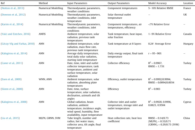
Table 1

Review summary of solar thermal system modelling techniques.

Ref Method Input Parameters Output Parameters Model Accuracy Location

(Notton et al., 2013) Numerical Modelling Thermodynamic parameters, weather conditions

Component temperatures 5e10% Relative RMSE France (Dowson et al., 2012) Numerical Modelling Thermodynamic parameters,

weather conditions, inlet temperature

Solar thermal outlet temperature

e UK

(Karim et al., 2014) Numerical Modelling Thermodynamic parameters, weather conditions, inlet conditions

Component temperatures, air temperatures, efﬁciency

<7% Relative Error e

(Yaïci and Entchev, 2016) ANFIS Ambient temperature, solar radiation, previous tank temperatures

Tank temperature, heat input, solar fraction

1e9% Relative Error Canada

(Geczy-Víg and Farkas, 2010) ANN Ambient temperature, solar radiation, massﬂow rate, previous tank temperature

Tank temperature at 8 layers 0.24_{Average Error} _Hungary

(Kalogirou et al., 2014) ANN Average daily temperature, total daily solar radiation, starting tank temperature

Daily energy output,ﬁnal tank temperature

r¼95e96% e

(Caner et al., 2011) ANN Date, time, inlet and outlet collector temperature, tank temperature, ambient and surface temperature, solar radiation

Collector efﬁciency R2_¼_0.9967, RMSE¼1.73%

Turkey

(Esen et al., 2009) WNN, ANN Ambient temperature, solar radiation, absorbing plate temperatures

Efﬁciency, outlet temperature R2_¼_{0.9992/0.9994,} RMSE¼0.0094/0.0034

Turkey

(S€ozen et al., 2008) ANN Date, time, surface temperature, solar radiation, declination, azimuth and tilt angles

Efﬁciency R2_¼_0.983 _Turkey

(Kalogirou et al., 2008) ANN Global radiation, beam radiation, ambient

temperature, incidence angle, wind speed, humidity,ﬂow availability, input temperature

Collector inlet and outlet temperature, storage inlet and outlet temperature

R2_¼_{0.9920, 0.9996,} 0.8823, 0.9504

Cyprus

(Liu et al., 2015) MLFN, GRNN, SVM Tube length, number and radius, hot water mass, collector area, tilt angle,ﬁnal temperature

Heat collection rate, heat loss coefﬁcient

RMSE¼0.14/0.73 (MLFN),¼0.33/0.71 (GRNN),¼0.29/0.73 (SVM)

China

Note - ANFIS (Adaptive Neuro-Fuzzy Inference System), ANN (Artiﬁcial Neural Network), WNN (Wavelet Neural Network), MLFN (Multi-Layer Feed-Forward Neural Network), GRNN (General Regression Neural Network), SVM (Support Vector Machine), RMSE (Root Mean Squared Error).

(4)

support vector regression (SVR). The work also does not take into account system control variables as input features, which increases the complexity of the problem. Furthermore, the models developed in this study can provide a 24-h ahead prediction of USTE at an hourly time-step rather than the total daily sum or parameters with limited applicability such as efﬁciency.

The research presented in this paper mainly addresses the following aspects;

the use of ensemble-based techniques for solar thermal systems as current application of machine learning algorithms are limited and most of the previous research work are focussed on artiﬁcial neural networks and its variants,

the use of tree-based ensemble methods to provide insight into the analysis of the variable importance of each input feature, i.e. using them as feature selection tools. In most of the existing research, domain knowledge is widely used to reduce input variable space. The presented analysis will allow researchers to gain better understanding of the modelled systems, and, to demonstrate that tree-based ensemble methods can improve

the prediction and stability of the developed model. Also, they are more computationally efﬁcient as compared to the con-ventional methods used in the literature (for example, support vector regression in our case).

The rest of the paper is organised as follows: Section2describes the principles of random forest, extra trees, decision trees and support vector regression. The methodology of the developed prediction models is presented in Section 3, along with feature selection process and results. Prediction results and discussion are detailed in Section 4, whereas concluding remarks and future research directions are presented at the end of the paper.

2. Machine learning methods

Four data-driven algorithms for predicting useful solar thermal energy are introduced in this section. These algorithms include extra trees (ET), random forest, decision trees, and support vector regression (SVR).

2.1. Support vector machines

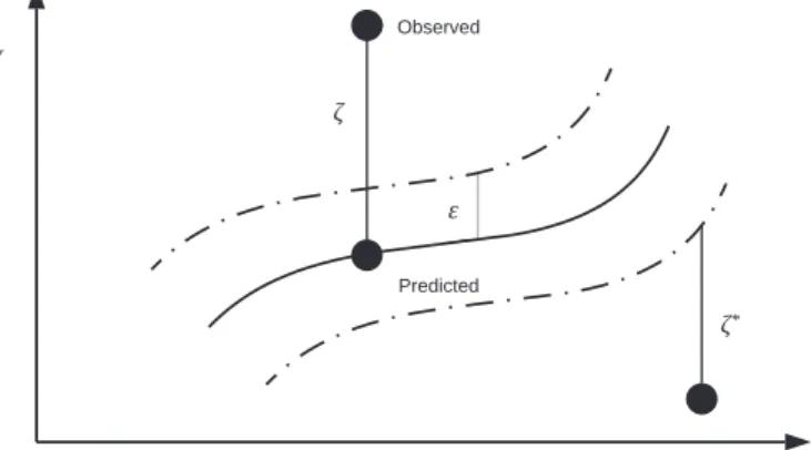
Support vector machine is one of the most widely used computational intelligence technique applied in building energy and renewable energy generation prediction and modelling appli-cations. It provides a sparse pattern of solutions andflexible control on the model complexity (Deng et al., 2018), making it highly effective in solving non-linear problems even with a small sample of training datasets. SVM adopts the structure risk minimisation (SRM) principle; which instead of only minimising the training error (this the principle of traditional empirical risk minimisation), minimises an upper bound of the generalisation error consisting of the sum of the training error and a confidence interval (Dong et al., 2005). SVM is commonly applied with different kernel functions to map the input space into a higher dimensional feature space, which introduces the non-linearity in the solution, and to perform a linear regression in the feature space (Li et al., 2009; Vapnik, 2013). Assuming normalised input variables consist of a vectorXi, andYiis the useful solar thermal energy (irepresents theith_{data-point in} the dataset). In this case, a set of data points can be defined as fðXi;YiÞgNi¼1, where Nis the total number of samples. An SVM regression approximates the function using the form given in Equation(1)(Dong et al., 2005;LIN et al., 2006).

Y¼fðXÞ ¼W$∅ðXÞ þb (1)

In Equation (1), ∅ðXÞ denotes the high-dimensional space. A regularised risk function, given in Equation(2), is used to estimate coefﬁcientsWandb(Li et al., 2009).

Minimise:1₂kWk2_þ_C1 N XN i¼1 LεðYi;fðXiÞÞ (2) LεðYi;fðXiÞÞ ¼ 0; jY_ifðX_iÞj ε jYifðXiÞj ε; others (3)

a

i;

a

i2 0;C

In Equation (5)

a

i;

a

i are Lagrange multipliers, i and j are different samples. Therefore, Equation(1)becomes (Li et al., 2009);

Fig. 1.The parameters of the support vector regression. Source (Dong et al., 2005;Li et al., 2009).

(5)

Y¼fðXÞ ¼XN i¼1

_a

i

a

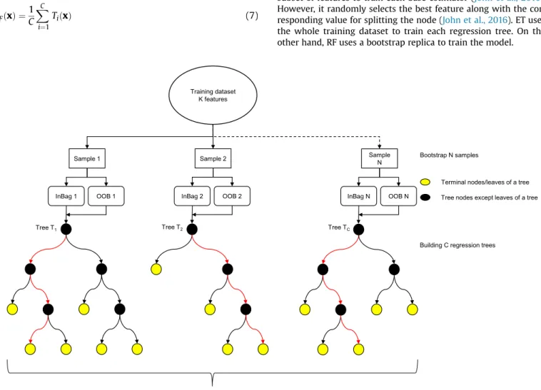
i kXi;Xj þb (6) 2.2. Random forest

A random forest (RF) is a tree-based ensemble method and was developed to address the shortcomings of traditional Classification and Regression Tree (CART) method. RF consists of a large number of weak decision tree learners, which are grown in parallel to reduce the bias and variance of the model at the same time (Breiman, 2001). For training a random forest, N bootstrapped sample sets are drawn from the original dataset. Each bootstrapped sample is then used to grow an unpruned regression (or classifi -cation) tree. Instead of using all available predictors in this step, only a small andfixed number of randomly sampledKpredictor are selected as split candidates. These two steps are then repeated until Csuch trees are grown, and new data is predicted by aggregating the prediction of theCtrees. RF uses bagging to increase the di-versity of the trees by growing them from different training data-sets, and hence reducing the overall variance of the model (Rodriguez-Galiano et al., 2015). A RF regression predictor can be expressed as; b_fC RFðxÞ ¼ 1 C XC i¼1 TiðxÞ (7)

wherexis the vectored input variable, C is the number of trees, and TiðxÞis a single regression tree constructed based on a subset of input variables and the bootstrapped samples. RF can natively perform out-of-bag error estimation in the process of constructing the forest by using the samples that are not selected during the training of thei-thtree in the bagging process. This subset is called out-of-bag, which can compute an unbiased estimation of gener-alisation error without using an external text data subset (Breiman, 2001). RF also enables assessment of relative importance of input features, which is useful for dimensionality reduction to improve model's performance on high-dimensional datasets (Ahmad et al., 2017). The RF switches one of the input variables while keeping the remaining constant, and measures the mean decrease in model's prediction accuracy, which is then used to assign relative importance score for each input variable (Breiman, 2001).Fig. 2 shows the structure of random forest algorithm.

2.3. Extra trees

Extremely randomised trees (or extra trees) (Geurts et al., 2006) algorithm is a relatively recent machine learning techniques and was developed as an extension of random forest algorithm, and is less likely to overﬁt a dataset (Geurts et al., 2006). Extra tree (ET) employs the same principle as random forest and uses a random subset of features to train each base estimator (John et al., 2016). However, it randomly selects the best feature along with the cor-responding value for splitting the node (John et al., 2016). ET uses the whole training dataset to train each regression tree. On the other hand, RF uses a bootstrap replica to train the model.

(6)

2.4. Decision trees

A decision tree (DT) is an efﬁcient algorithm for classiﬁcation and regression problems. The basic idea of the decision tree algo-rithm is to split a complex problem into several simpler problems, which might lead to a solution that is easier to interpret (Xu et al., 2005). A DT represents a set of conditions, which are hierarchically organised and successively applied from root to leaf of the tree (Breiman et al., 1984). DTs are easy to interpret and their structure is transparent. DTs produce a trained model that can represent logical rules, which can then be used to predict new dataset through the repetitive process of splitting (Ahmad et al., 2017). According to Breiman et al. (1984); in a decision tree method, features of data are referred as predictor variables whereas the class to be mapped is the target variable. For regression problems, the target variables are continuous.

To train a DT model, recursive partitioning and multiple re-gressions are performed from the training dataset. From the root node of the tree, the data splitting process in each internal node of a rule of the tree is repeated until the stopping criterion is met (Rodriguez-Galiano et al., 2015). In DT algorithm, each leaf node of the tree contains a simple regression model, which only applies to that leaf only. After the induction process, pruning can be applied to improve the generalisation capability of the model by reducing the tree's complexity (Rodriguez-Galiano et al., 2015). For a solar thermal collector application, a simple example of decision tree to predict USTE is depicted inFig. 3. The output of the decision tree is the useful solar thermal energy. It is worth mentioning that the decision tree is only for demonstration purpose and the actual DT used in the analysis is more complex (i.e., more than two features are considered when looking for best split and the tree is deeper). The decision tree shown inFig. 3only considers solar radiation and outdoor dry-bulb air temperature as input variables, and the maximum depth of the tree is restricted to 3.

3. Material and methods

This section details the training and testing datasets, feature selection process and results. The section also details metrics used for assessing models’predictive performance. The implementation of extra trees, random forest, support vector regression included in the scikit-learn (Pedregosa et al., 2011) module of python pro-gramming language was used for all developmental and experi-mental work. The work was carried out on a personal computer (Intel Core i5 2.50 GHz with 16 GB of RAM).

3.1. Data description

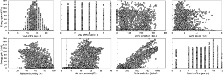
The studied solar thermal system is installed at an experimental facility in Chambery, France and has a total area of 400 m 2. The solar loop contains a mixture of 60% and 40% water-glycol, and has a density of 1044 kg/m3. The mass ﬂow rate, supply and return temperatures are monitored every minute. The building also has an on-site weather station; which monitors outdoor dry-bulb air temperature, solar radiation, wind speed and direction, relative humidity and atmospheric pressure. In total, after removing out-liers and missing values, the training and testing datasets contained 5580 data samples. The data was collected from 01st April 2017 to 25th January 2018. Predicting USTE is a challenging task as none of the system variables (i.e. massﬂow rate, supply and return tem-perature) are considered as input variables. The system variables are not available in advance and therefore are not suitable for future predictions (unless separate models are developed for those vari-ables). Also, USTE did not exhibit any clear pattern as opposed to solar PV prediction (which is almost directly related to solar radi-ation), as it would also depend on energy load on thermal storage. Training data is taken as 70% of the whole dataset, and remaining data samples were used as testing dataset.Fig. 4displays the scatter plots for each of the input variables with USTE. It is clear that any

(7)

relationship of input features and the output variable is not trivial, and simple learners may not be able to accurately predict USTE. It is also important to mention that features were normalised before applying SVR to avoid features in greater numeric ranges domi-nating those in smaller numeric ranges. In this paper, we will focus on developing machine learning models for useful solar thermal energy (Qc), without using system controlled and uncontrolled variables (i.e. massﬂow rate, and supply and return temperature). The absorption heat transfer rate or USTE,Q_c, can be calculated by using Equation(8)(Karsli, 2007).

_

Qc¼m_Cp ðToutTinÞ (8)

In Equation(8),m_ is the massflow rate,Cpis the specific heat of the solar collector_fluid, andTin andTout are the inlet and outlet temperatures of the solar collector.

3.2. Uncertainty analysis

To assess the performance of developed models on training and testing datasets; root mean square error (RMSE), mean absolute error (MAE) and the determination coefﬁcient (R2) were calculated. The determination coefﬁcient was adopted to measure the corre-lation between the actual and estimated USTE values. The former

two indicators are deﬁned as below;

RMSE¼ ffiffiffiffiffiffiffiffiffiffiffiffiffiffiffiffiffiffiffiffiffiffiffiffiffiffiffi PN i¼1 ðyibyiÞ2 N v u u u t (9) MAE¼1 N XN i¼1 jbyiyij (10)

whereby_iis the predicted value,y_iis the actual value, and N is the total number of samples. In this work, root mean squared error (RMSE) is used as the primary metric.

3.3. Feature subset selection

Feature selection is an important step in the development of machine learning models. The number of input features may vary from two to hundreds of features, among them many may be un-important or have lower correlation with the target variables. Previous research works have demonstrated that prediction models are often affected by high variance in the training dataset (Neupane et al., Aung). Feature selection methods increase models' performance on high-dimensional datasets by reducing training time, enhancing model's generalization capability, improving interpretability of the models (Ahmad et al., 2017). Random forest and extra trees also allow the estimation of the importance of each feature in the model.Fig. 5shows the results of internal calculation carried out by ET and RF algorithms, as well as features' Pearson correlation with hourly useful thermal energy gain. It is interesting to notice that each of the machine learning models has different variable importance score for some of the input features. As an example; for the ET model, outdoor relative humidity has a variable importance score of 0.072. Whereas, RF has a low score for relative humidity (i.e. 0.0058). Solar radiation was considered as the most important feature by both algorithms. As expected, Outdoor dry-bulb air temperature, solar radiation and hour of the day present a positive correlation with the useful solar thermal energy, as demonstrated by their Pearson correlation coefﬁcients. On the other hand, outdoor relative humidity, wind speed, wind direction, the month of the year and atmospheric pressure are negatively related to the useful solar thermal energy. Later in the results, we will discuss that the prediction of USTE could be improved by integrating demand load prediction. The prediction could also be

Fig. 4.Scatter plot demonstrating the relation between input and output variables.

Fig. 5.Feature importance and Pearson correlation for solar thermal useful energy prediction. Notes: Pres.: atmospheric pressure, Mon: month of the year, Day: day of the week, Hr: hour of the day, WD: wind direction, WS: wind speed, Rad: Solar radiation, RH: Outdoor air relative humidity, DBT: outdoor air dry-bulb temperature.

(8)

improved by considering previous hour useful solar thermal en-ergy. However, in the current work, previous hour values are not considered and will need to be investigated in future.

4. Prediction results and discussion

This section details the prediction results obtained with tree-based ensemble machine learning methods (random forest and extra trees), support vector regression and decision trees; which are described in Section2. This section also details an assessment of the impact of different hyper-parameters on model's performance.

4.1. Hyper-parametric tuning

Model's hyper-parameters has a great inﬂuence on its predictive performance, robustness and generalization capability. This section details the selection of optimal hyper-parameters of studied algo-rithms. For this purpose, a stepwise searching method is used to

find optimal values of model's hyper-parameters. In order to pre-vent over-_fitting problems and analyse models' performance on unknown data, a cross-validation approach is used to select optimal hyper-parameters. In k-fold cross-validation, the training dataset is divided into k subsets of equal size. Each k subset is used as a validation dataset, whereas the remaining k-1 subsets are used as training dataset. In this study,five-fold validation is performed for selecting optimal hyper-parameters.

4.1.1. Support vector regression

Different factors affect the generalisation capabilities of support vector regression, i.e. to predict unseen data after learning carried out on training dataset. SVR needs the adjustment of (a) kernel functionelinear, polynomial, sigmoid and radial-basis (RBF); (b) gamma of the kernel function, except for linear kernel function; (c) degree of the polynomial kernel function; (d) bias on the kernel function, only applicable to the sigmoid and polynomial kernels; (e) penalty parameter (C) of the error term and; (f) radius (ε). These parameters need to be tuned to make sure that the developed models do not underﬁt or overﬁt data.

In the literature, RBF kernel has been widely used for regression problems as it non-linearly maps samples into a high dimensional space, and can easily handle the non-linear relationship between class labels and attributes (Dong et al., 2005). A polynomial kernel function has more hyper-parameters to tune as compared to RBF. Due to its wide use and lower complexity (fewer hyper-parameters to consider), RBF was selected for this study. For RBF, there are three hyper-parameters to tune, i.e., kernel coefﬁcient (

g

), penalty parameter of the error term (C) and radius (ε). According to the deﬁnition of the kernel coefﬁcient byChang and Lin (2011),

g

¼

1=K, where K is the number of input features. Therefore, for this paper,

g

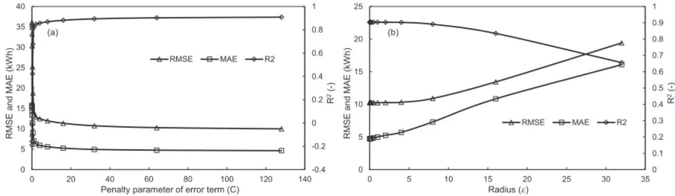
¼1/5 was used to estimate outlet temperature and useful energy from a solar thermal heating system. Penalty parameter (C) of the error term is used tofind the trade-off between the model complexity and the degree to which deviations larger thanεare tolerated in the optimisation formulation (represented by Equation (4)). A small value of C will place a small weight on the training data and therefore will result in an under-fit model. On the contrary, a too large value of C will only minimise the empirical risk, and hence will under-fit the training dataset. In this study, a step wise search was used tofind optimal values of C andε. Initially,εwasfixed at 0.1 while varyingCover the range of 27and 27. From results inFig. 6, it is evident that initially there was significant improvement in the performance of the model with an increase of C. However, from the results, it was found that higher values of C did not significantly improve the performance and also it was computationally intensive process to train SVR with larger C values. Therefore, a value of C¼26 was selected for further experiments. Too large values of parameter ε also deteriorate model's accuracy as it controls the width of theε-intensive zone (Dong et al., 2005). Values ofεwere varied over the range of 210 and 25, while keepingC¼26. It is evident fromFig. 6that larger values drastically reduce the accu-racy of the model. From the results, a value ofε¼27was selected as it provided best results.

4.1.2. Random forest, extra trees and decision trees

Tree-based ensemble methods (extra trees and random forest) need the adjustment of three hyper-parameters, i.e. number of trees (M), number of minimum samples required for splitting a node (nmin) and attribute selection strength parameter (K). ParameterMrepresents the total number of trees in the forest and is directly related to the computational cost. Therefore, a reason-able number of trees need to be selected toﬁnd a trade-off between predictive power and computational time. For this paper, 100 number of trees were selected in the forest as increasing the number of trees to greater than 100 did not signiﬁcantly improve prediction results. K denotes the number of randomly selected features at each node during the tree growing process, and de-termines the strength of variable selection process. For most regression problems, this parameter is set to p, wherep is the dimension of input features vector (Geurts et al., 2006).

For ET, DT and RF, it was found thatnmin did not signiﬁcantly enhance the performance of the models and therefore a default value of 2 was selected for this parameter. K values were varied in the range of (Ahmad et al., 2016a; Kalogirou, 2004) (i.e. total numbers of features selected for model construction process). For ET and DT,K¼5 resulted in better results. Whereas, for RF,K¼2 produced optimal results. It is worth mentioning that for RF and ET,

(9)

Kparameter did not drastically enhance the results. On the con-trary; for DT,Ksigniﬁcantly enhance the prediction results, i.e. for values ofKequals to 1 and 5, models has R2values of 0.8577 and 0.9140, respectively. Table 2 shows the dependence of models’

performance on maximum tree depth. Generally, deeper trees resulted in better performance. For ET and RF, trees deeper than 10 started to deteriorate and led to under-ﬁtting. A maximum depth of 5 levels produced marginally better results for DT. From the results, it is evident that for the studied tree-based ensemble algorithms, default parameters are near-optimal and could result in a robust prediction model.

4.2. Model analytical results

Table 3presents the RMSE, R2, and MAE on training and testing datasets for predicting USTE. Generally, errors on the testing dataset show the generalisation capabilities of the developed models. On the other hand, errors on the training dataset show the goodness-of-ﬁt of the developed models. Results inTable 3suggest that RF and ET achieved the best performance across training and testing datasets. RF achieved RMSE values of 3.96 and 6.86 on training and testing datasets, respectively. Whereas, ET has RMSE values of 3.79 on training and 7.12 on testing datasets. The results

Table 2

Results of various dminfor ET, RF and DT.

dmin Extra trees Random forest Decision Tree

R2₍₎ _{RMSE (kWh)} _{MAE (kWh)} _R2₍₎ _{RMSE (kWh)} _{MAE (kWh)} _R2₍₎ _{RMSE (kWh)} _{MAE (kWh)}

1 0.7634 16.1055 10.5532 0.5226 22.8774 15.9858 0.7819 15.4619 8.6532 3 0.8944 10.7576 5.1266 0.8982 10.5639 5.9474 0.9081 10.0368 4.5962 5 0.9317 8.6529 3.8446 0.9397 8.1295 4.0182 0.9300 8.7570 3.4668 7 0.9443 7.8122 3.3374 0.9513 7.3028 3.2673 0.9248 9.0782 3.4126 9 0.9523 7.2327 2.9462 0.9552 7.0041 3.0218 0.9239 9.1292 3.3824 10 0.9538 7.1187 2.8737 0.9570 6.8647 2.9168 0.9239 9.1322 3.3420 11 0.9536 7.1287 2.8534 0.9570 6.8660 2.8971 0.9184 9.4566 3.4448 12 0.9537 7.1252 2.8249 0.9560 6.9443 2.9236 0.9201 9.3552 3.3994 13 0.9529 7.1854 2.8382 0.9567 6.8874 2.8882 0.9194 9.3982 3.4511 15 0.9524 7.2227 2.8225 0.9570 6.8680 2.8643 0.9173 9.5232 3.5334 20 0.9526 7.2080 2.8242 0.9553 7.0002 2.8986 0.9099 9.9370 3.6294

NoteseFor RF:nmin ¼2,K¼2,M¼100; for ET:nmin¼2,K¼5,M¼100; and for DT:nmin¼2,K¼5.

Table 3

Comparison of models on full training and testing datasets.

Model Training dataset Testing dataset Training time (ms)

R2₍₎ _{RMSE (kWh)} _{MAE (kWh)} _R2₍₎ _{RMSE (kWh)} _{MAE (kWh)}

DT 0.957 6.780 2.908 0.930 8.758 3.467 16.00

ET 0.987 3.791 1.630 0.954 7.119 2.874 421.00

SVR 0.917 9.460 4.459 0.903 10.287 4.755 1287.80

RF 0.985 3.955 1.796 0.957 6.8651 2.917 491.60

(10)

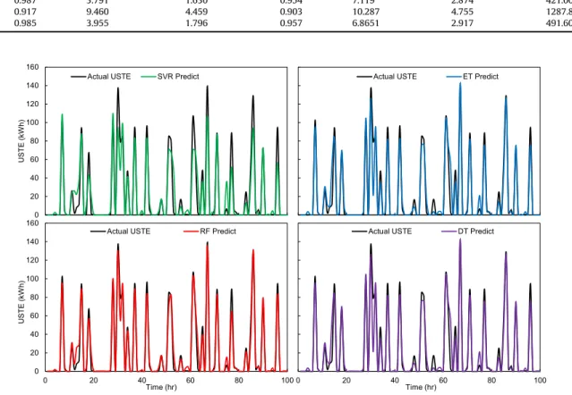
showed that tree-based ensemble methods have nearly compara-ble performance. SVR has the highest training and testing errors, while DT has achieved marginally better performance as compared to SVR.Fig. 7illustrates the plot for hourly USTE values predicted by all studied machine learning models vs measured data. It can be concluded that both ET and RF showed strong non-linear mapping generalisation ability, and can be effective in predicting hourly USTE. It was found that best performing methods, RF and ET, over predicted some of the values. Even though the solar radiation values were higher and it was expected to have higher values of USTE. However, the difference between supply and return tem-perature was small, and therefore the actual value of USTE was lower. In the future work, this problem will need to be tackled, and it is envisaged that considering thermal load on the storage tank as an input variable will further improve models' accuracy. SVR al-gorithm did not capture the peaks values of USTE and therefore produced worse results as compared to other algorithms. RF closely followed the USTE pattern and therefore performed better on the testing dataset. Also, ET algorithm had the lowest training time (421 ms) than RF (491.60 ms) and SVR (1287.80 ms). Among all studied algorithms, DT was found to be the least computationally intensive. However, this comes at the expense of model's accuracy, as DT has a lower training and testing performances as compared to ET and RF.

4.3. Number of training samples

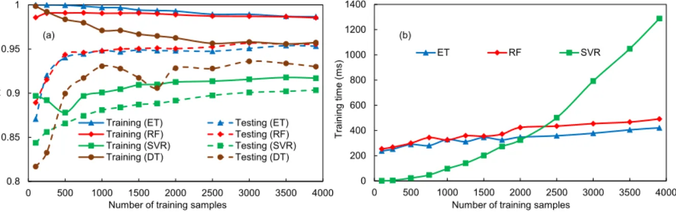
The number of training samples has two impacts on machine learning algorithms; 1) with the increase in the number of training samples, it is expected that the training time and memory usage during the training phase will increase, and 2) it will increase prediction accuracy of the model. It is worth mentioning here that the training time could also depend on many factors, e.g the implementation of an algorithm in the programming library, number of input features used, model complexity, feature extrac-tion, input data representation and sparsity (Ahmad et al., 2017). For tree-based ensemble methods, this would also depend on other factors, e.g. number of trees in the forest, maximum depth of a tree, etc. (Ahmad et al., 2017). To demonstrate the sensitivity of machine learning models to the training dataset size and time required to construct a model, different experiments were performed.Fig. 8(a) shows the effect of the number of training data samples on models' predictive performance. Generally, all developed models react in a gradual way to an increase in the training sample size. For all studied algorithms, it was found that increasing the number of samples increases the models' generalisation ability (i.e., increased performance on the unseen testing dataset). It can be seen inFig. 8

that both RF and ET showed almost same behaviour on training and testing datasets. Their accuracy signiﬁcantly increased between n¼100 and n¼500. SVR showed relatively lower accuracy on both training and testing datasets as compared to ET, RF, and DT. It is also important to mention that for tree-based algorithms; the accuracy on training dataset reduced with an increase in the training dataset. For SVR; initially there was a decrease in the accuracy on training dataset, which started to increase after n¼500.Fig. 8(b) shows the SVR has signiﬁcantly higher training time as compared to RF and ET. Please note that DT training time is considerably small and there-fore we have not considered it in Fig. 8(b). SVR training time increased exponentially with an increase in the training data samples. ET and RF algorithms have comparable training time on lower number of training samples. However, RF has marginally higher training time for n>1500. In this work, we analysed the impact of number of samples on models' performance and training time. However, in future, training time dependency on algorithm's hyper-parameter will be explored.

5. Conclusions

The paper details the feasibility of using machine learning al-gorithms to predict hourly useful solar thermal energy. For this purpose, a solar thermal system installed at Chambery, France was used as a case study. Experiments were performed over the period of April 2017 through January 2018 to gather experimental data for training and testing machine learning models. Different statistical measures were used to appraise the models’ prediction perfor-mance. The capability of decision tree-based ensemble methods for predicting the USTE has been veriﬁed with better accuracy as compared to decision trees and support vector regression. The re-sults also demonstrated that ET and RF algorithms have signiﬁ -cantly lower training time, i.e., 421 ms and 491.60 ms, respectively as compared to 1287.80 ms for SVR.

The developed tree-based ensemble methods improved the prediction results and have RMSE values of 6.87 and 7.12 for RF and ET, respectively. Both of these methods were developed to over-come shortcomings of CART, e.g.ﬁnal tree is not guaranteed to be the optimal tree and generate a stable model. Simple regression trees are not effective for predicting hourly USTE. However, en-sembles of these trees have signiﬁcantly improved models’ per-formance. Tree-based ensemble methods discussed in this paper require fewer tuning parameters and in most cases default hyper-parameters can result in satisfactory performance. The developed models only used weather and time information to predict hourly USTE. To the best of our knowledge, previous works also considered system control variables as inputs to the model. The system

(11)

variables are not available in advance and therefore are not suitable for future predictions (unless separate models are developed for these variables). The developed tree-based ensemble methods can achieve accurate and reliable hourly prediction and could be used for fault detection and diagnosis (e.g., solar collector fault, shaded collector area, value fault, etc.), making informed decisions and operational optimisation of multi-vector energy systems. In future work, another promising emerging technique, deep learning, will need to be investigated for solar thermal collectors. Machine learning models for different types of solar collectors and solar collector based systems will need to be developed to cover a wide range of systems. The performance of models will be enhanced in future by incorporating storage load predictions.

Acknowledgement

The work was carried out in the framework of the Horizon 2020 project (Grant reference e731125) PENTAGON00Unlocking Euro-pean grid local ﬂexibility trough augmented energy conversion capabilities at district-level”. The authors acknowledge theﬁ nan-cial support from the European Commission. The authors also like to thank Michael Descamps (CEA-INES) for providing valuable experimental data. Nomenclature

z

1,

z

1 slack variables

a

i;

a

i Lagrange multipliers kwk2 _{Euclidean norm} kðXi;XjÞ kernel function ε precision parameter/radius C Number of trees/penalty parameter

g

RBF kernel coefﬁcient

M number of trees in a forest x inputs

N number of training samples for SVR Cp speciﬁc heat

Tout outlet temperature of the solar collector

Abbreviations

ANFIS adaptive neuro-fuzzy inference system CART classiﬁcation and regression trees ET extra trees

MAE mean absolute error RBF radial basis function RF random forest

SVR support vector regression WNN wavelet neural network b bias term

nmin number of minimum samples required for splitting a tree node

∅ðxÞ non-linear transformation W weight vector

Ti regression tree

bfC_RF random forest regression predictor K attribute selection parameter N number of training samples y outputs

_

m massﬂow rate

Tin inlet temperature of the solar collector ANN artiﬁcial neural network

DT decision tree

GRNN general regression neural network PV photovoltaic

RES renewable energy resources RMSE root mean square error USTE useful solar thermal energy

References

Ahmad, M.W., Mourshed, M., Mundow, D., Sisinni, M., Rezgui, Y., 2016a. Building energy metering and environmental monitoringe a state-of-the-art review and directions for future research. Energy Build. 120 (Suppl. C), 85e102. ISSN 0378-7788, secondoftwo doi:https://doi.org/10.1016/j.enbuild.2016.03.059. Ahmad, M.W., Mourshed, M., Yuce, B., Rezgui, Y., 2016b. Computational intelligence

techniques for HVAC systems: a review. Building Simulation 9 (4), 359e398. https://doi.org/10.1007/s12273-016-0285-4secondoftwo doi:

Ahmad, M.W., Mourshed, M., Rezgui, Y., 2017. Trees vs Neurons: comparison be-tween random forest and ANN for high-resolution prediction of building energy consumption. Energy Build. 147 (Suppl. C), 77e89.https://doi.org/10.1016/ j.enbuild.2017.04.038. ISSN 0378-7788, secondoftwo doi:

Benedetti, M., Cesarotti, V., Introna, V., Serranti, J., 2016. Energy consumption control automation using Artiﬁcial Neural Networks and adaptive algorithms: proposal of a new methodology and case study. Appl. Energy 165, 60e71. https://doi.org/10.1016/j.apenergy.2015.12.066secondoftwo doi:

Breiman, L., 2001. Random forests. Mach. Learn. 45 (1), 5e32.

Breiman, L., Friedman, J., Stone, C.J., Olshen, R.A., 1984. Classiﬁcation and Regression Trees. CRC press.

Breiman, L., et al., 1996. Heuristics of instability and stabilization in model selection. Ann. Stat. 24 (6), 2350e2383.

Cadenas, E., Rivera, W., 2009. Short term wind speed forecasting in La Venta, Oaxaca, Mexico, using artiﬁcial neural networks. Renew. Energy 34 (1), 274e278.https://doi.org/10.1016/j.renene.2008.03.014secondoftwo doi: Caner, M., Gedik, E., Keçebas¸, A., 2011. Investigation on thermal performance

calculation of two type solar air collectors using artiﬁcial neural network. Expert Syst. Appl. 38 (3), 1668e1674.https://doi.org/10.1016/j.eswa.2010.07.090 secondoftwo doi:

Catal~ao, J. P. d. S., Pousinho, H.M.I., Mendes, V.M.F., 2011. Short-term wind power forecasting in Portugal by neural networks and wavelet transform. Renew. Energy 36 (4), 1245e1251. https://doi.org/10.1016/j.renene.2010.09.016 sec-ondoftwo doi:

Chae, Y.T., Horesh, R., Hwang, Y., Lee, Y.M., 2016. Artiﬁcial neural network model for forecasting sub-hourly electricity usage in commercial buildings. Energy Build. 111, 184e194.https://doi.org/10.1016/j.enbuild.2015.11.045secondoftwo doi: Chang, C.-C., Lin, C.-J., 2011. LIBSVM: a library for support vector machines. ACM

Trans. Intell. Syst. Technol. (TIST) 2 (3), 27.

Deng, H., Fannon, D., Eckelman, M.J., 2018. Predictive modeling for US commercial building energy use: a comparison of existing statistical and machine learning algorithms using CBECS microdata. Energy Build. 163, 34e43.https://doi.org/ 10.1016/j.enbuild.2017.12.031. ISSN 0378-7788, secondoftwo doi:

Dietterich, T.G., 2000. Ensemble methods in machine learning. In: International Workshop on Multiple Classiﬁer Systems, vols. 1e15. Springer.

Dong, B., Cao, C., Lee, S.E., 2005. Applying support vector machines to predict building energy consumption in tropical region. Energy Build. 37 (5), 545e553. https://doi.org/10.1016/j.enbuild.2004.09.009. ISSN 0378-7788, secondoftwo doi:

Dowson, M., Pegg, I., Harrison, D., Dehouche, Z., 2012. Predicted and in situ per-formance of a solar air collector incorporating a translucent granular aerogel cover. Energy Build. 49, 173e187.https://doi.org/10.1016/j.enbuild.2012.02.007 secondoftwo doi:

Dufﬁe, J.A., Beckman, W.A., 2013. Solar Engineering of Thermal Processes. John Wiley&Sons.

Esen, H., Ozgen, F., Esen, M., Sengur, A., 2009. Artiﬁcial neural network and wavelet neural network approaches for modelling of a solar air heater. Expert Syst. Appl. 36 (8), 11240e11248.https://doi.org/10.1016/j.eswa.2009.02.073secondoftwo doi:

Eurostat, 2016. Primary Production of Renewable Energy by Type. URL.http://ec. europa.eu/eurostat/web/energy/data/main-tables.

Fan, C., Xiao, F., Wang, S., 2014. Development of prediction models for next-day building energy consumption and peak power demand using data mining techniques. Appl. Energy 127, 1e10. https://doi.org/10.1016/j.ape-nergy.2014.04.016secondoftwo doi:

Geczy-Víg, P., Farkas, I., 2010. Neural network modelling of thermal stratiﬁcation in a solar DHW storage. Sol. Energy 84 (5), 801e806.https://doi.org/10.1016/ j.solener.2010.02.003secondoftwo doi:

Geurts, P., Ernst, D., Wehenkel, L., 2006. Extremely randomized trees. Mach. Learn. 63 (1), 3e42.https://doi.org/10.1007/s10994-006-6226-1secondoftwo doi: Hansen, L.K., Salamon, P., 1990. Neural network ensembles. IEEE Trans. Pattern Anal.

Mach. Intell. 12 (10), 993e1001.https://doi.org/10.1109/34.58871secondoftwo doi:

John, V., Liu, Z., Guo, C., Mita, S., Kidono, K., 2016. Real-time Lane Estimation Using Deep Features and Extra Trees Regression. Springer International Publishing, Cham, pp. 721e733. https://doi.org/10.1007/978-3-319-29451-3_57 sec-ondoftwo doi:

Kalogirou, S.A., 2004. Solar thermal collectors and applications. Prog. Energy Combust. Sci. 30 (3), 231e295. ISSN 0360-1285, secondoftwo doi.https://doi. org/10.1016/j.pecs.2004.02.001.

(12)

Kalogirou, S., Lalot, S., Florides, G., Desmet, B., 2008. Development of a neural network-based fault diagnostic system for solar thermal applications. Sol. En-ergy 82 (2), 164e172.https://doi.org/10.1016/j.solener.2007.06.010secondoftwo doi:

Kalogirou, S., Mathioulakis, E., Belessiotis, V., 2014. Artiﬁcial neural networks for the performance prediction of large solar systems. Renew. Energy 63, 90e97. https://doi.org/10.1016/j.renene.2013.08.049secondoftwo doi:

Karim, M., Perez, E., Amin, Z.M., 2014. Mathematical modelling of counterﬂow v-grove solar air collector. Renew. Energy 67, 192e201.https://doi.org/10.1016/ j.renene.2013.11.027secondoftwo doi:

Karsli, S., 2007. Performance analysis of new-design solar air collectors for drying applications. Renew. Energy 32 (10), 1645e1660. https://doi.org/10.1016/ j.renene.2006.08.005. ISSN 0960-1481, secondoftwo doi:

Kharb, R.K., Shimi, S., Chatterji, S., Ansari, M.F., 2014. Modeling of solar PV module and maximum power point tracking using ANFIS. Renew. Sustain. Energy Rev. 33, 602e612.https://doi.org/10.1016/j.rser.2014.02.014secondoftwo doi: Kusiak, A., Zheng, H., Song, Z., 2009. Short-term prediction of wind farm power: a

data mining approach. IEEE Trans. Energy Convers. 24 (1), 125e136.https:// doi.org/10.1109/TEC.2008.2006552secondoftwo doi:

Li, Q., Meng, Q., Cai, J., Yoshino, H., Mochida, A., 2009. Applying support vector machine to predict hourly cooling load in the building. Appl. Energy 86 (10), 2249e2256. https://doi.org/10.1016/j.apenergy.2008.11.035. ISSN 0306-2619, secondoftwo doi:

LIN, J.-Y., CHENG, C.-T., CHAU, K.-W., 2006. Using support vector machines for long-term discharge prediction. Hydrol. Sci. J. 51 (4), 599e612. https://doi.org/ 10.1623/hysj.51.4.599secondoftwo doi:

Liu, Z., Li, H., Zhang, X., Jin, G., Cheng, K., 2015. Novel method for measuring the heat collection rate and heat loss coefﬁcient of water-in-glass evacuated tube solar water heaters based on artiﬁcial neural networks and support vector machine. Energies 8 (8), 8814e8834.https://doi.org/10.3390/en8088814 secondoftwo doi:

Lund, H., Werner, S., Wiltshire, R., Svendsen, S., Thorsen, J.E., Hvelplund, F., Mathiesen, B.V., 2014. 4th Generation District Heating (4GDH): integrating smart thermal grids into future sustainable energy systems. Energy 68, 1e11. https://doi.org/10.1016/j.energy.2014.02.089. ISSN 0360-5442, secondoftwo doi:

Mathiesen, B.V., Lund, H., Connolly, D., Wenzel, H., Østergaard, P.A., M€oller, B., Nielsen, S., Ridjan, I., Karnøe, P., Sperling, K., Hvelplund, F.K., 2015. Smart Energy Systems for coherent 100% renewable energy and transport solutions. Appl. Energy 145, 139e154. ISSN 0306-2619, secondoftwo doi:https://doi.org/10. 1016/j.apenergy.2015.01.075.

Motte, F., Notton, G., Cristofari, C., Canaletti, J.-L., 2013. A building integrated solar collector: performances characterization andﬁrst stage of numerical calcula-tion. Renew. Energy 49, 1e5. https://doi.org/10.1016/j.renene.2012.04.049

secondoftwo doi:

B. Neupane, W. L. Woon, Z. Aung, Ensemble prediction model with expert selection for electricity price forecasting, Energies 10 (1).

Notton, G., Motte, F., Cristofari, C., Canaletti, J.-L., 2013. New patented solar thermal concept for high building integration: test and modeling. Energy Procedia 42, 43e52.https://doi.org/10.1016/j.egypro.2013.11.004secondoftwo doi: Pedregosa, F., Varoquaux, G., Gramfort, A., Michel, V., Thirion, B., Grisel, O.,

Blondel, M., Prettenhofer, P., Weiss, R., Dubourg, V., et al., 2011. Scikit-learn: machine learning in Python. J. Mach. Learn. Res. 12 (Oct), 2825e2830. Reynolds, J., Ahmad, M.W., Rezgui, Y., 2018. Holistic modelling techniques for the

operational optimisation of multi-vector energy systems. Energy Build. 169, 397e416.https://doi.org/10.1016/j.enbuild.2018.03.065. ISSN 0378-7788, sec-ondoftwo doi:

Rodriguez-Galiano, V., Sanchez-Castillo, M., Chica-Olmo, M., Chica-Rivas, M., 2015. Machine learning predictive models for mineral prospectivity: an evaluation of neural networks, random forest, regression trees and support vector machines. Ore Geol. Rev. 71 (804e818)https://doi.org/10.1016/j.oregeorev.2015.01.001. ISSN 0169-1368, secondoftwo doi:

J. L. Sawin, F. Sverrisson, K. Seyboth, R. Adib, H. E. Murdock, C. Lins, I. Edwards, M. Hullin, L. H. Nguyen, S. S. Prillianto, et al., reportRenewables 2017 Global Status Report .

S€ozen, A., Menlik, T., Ünvar, S., 2008. Determination of efﬁciency ofﬂat-plate solar collectors using neural network approach. Expert Syst. Appl. 35 (4), 1533e1539. https://doi.org/10.1016/j.eswa.2007.08.080secondoftwo doi:

Vapnik, V., 2013. The Nature of Statistical Learning Theory. Springer Science&

Business Media.

Wang, Z., Wang, Y., Zeng, R., Srinivasan, R.S., Ahrentzen, S., 2018. Random Forest based hourly building energy prediction. Energy Build. 171, 11e25.https:// doi.org/10.1016/j.enbuild.2018.04.008. ISSN 0378-7788, secondoftwo doi: Xu, M., Watanachaturaporn, P., Varshney, P.K., Arora, M.K., 2005. Decision tree

regression for soft classiﬁcation of remote sensing data. Rem. Sens. Environ. 97 (3), 322e336.https://doi.org/10.1016/j.rse.2005.05.008. ISSN 0034-4257, sec-ondoftwo doi:

Yaïci, W., Entchev, E., 2016. Adaptive Neuro-Fuzzy Inference System modelling for performance prediction of solar thermal energy system. Renew. Energy 86, 302e315.https://doi.org/10.1016/j.renene.2015.08.028secondoftwo doi: Yap, W.K., Karri, V., 2015. An off-grid hybrid PV/diesel model as a planning and

design tool, incorporating dynamic and ANN modelling techniques. Renew. Energy 78, 42e50. https://doi.org/10.1016/j.renene.2014.12.065 secondoftwo doi:

Yona, A., Senjyu, T., Saber, A.Y., Funabashi, T., Sekine, H., Kim, C.-H., 2007. Applica-tion of neural network to one-day-ahead 24 hours generating power fore-casting for photovoltaic system. In: Intenational Conference on Intelligent Systems Applications to Power Systems, 2007. ISAP 2007, vols. 1e6. IEEE (r).