Gene Selection and Classification for Cancer Microarray Data Based on Machine Learning and Similarity Measures

Based on Machine Learning and Similarity Measures

(Article begins on next page)

The Harvard community has made this article openly available.

Please share

how this access benefits you. Your story matters.

Citation

Liu, Qingzhong, Andrew H. Sung, Zhongxue Chen, Jianzhong

Liu, Lei Chen, Mengyu Qiao, Zhaohui Wang, Xudong Huang,

and Youping Deng. 2011. Gene selection and classification for

cancer microarray data based on machine learning and similarity

measures. BMC Genomics 12(Suppl. 5): S1.

Published Version

doi:10.1186/1471-2164-12-S5-S1

Accessed

February 19, 2015 9:55:30 AM EST

Citable Link

http://nrs.harvard.edu/urn-3:HUL.InstRepos:10318285

Terms of Use

This article was downloaded from Harvard University's DASH

repository, and is made available under the terms and conditions

applicable to Other Posted Material, as set forth at

http://nrs.harvard.edu/urn-3:HUL.InstRepos:dash.current.terms-of-use#LAA

R E S E A R C H

Open Access

Gene selection and classification for cancer

microarray data based on machine learning and

similarity measures

Qingzhong Liu

, Andrew H Sung

, Zhongxue Chen

, Jianzhong Liu

, Lei Chen

, Mengyu Qiao

, Zhaohui Wang

,

Xudong Huang

, Youping Deng

From

BIOCOMP 2010. The 2010 International Conference on Bioinformatics and Computational Biology

Las Vegas, NV, USA. 12-15 July 2010

Abstract

Background:Microarray data have a high dimension of variables and a small sample size. In microarray data analyses, two important issues are how to choose genes, which provide reliable and good prediction for disease status, and how to determine the final gene set that is best for classification. Associations among genetic markers mean one can exploit information redundancy to potentially reduce classification cost in terms of time and money.

Results:To deal with redundant information and improve classification, we propose a gene selection method, Recursive Feature Addition, which combines supervised learning and statistical similarity measures. To determine the final optimal gene set for prediction and classification, we propose an algorithm, Lagging Prediction Peephole Optimization. By using six benchmark microarray gene expression data sets, we compared Recursive Feature Addition with recently developed gene selection methods: Support Vector Machine Recursive Feature Elimination, Leave-One-Out Calculation Sequential Forward Selection and several others.

Conclusions:On average, with the use of popular learning machines including Nearest Mean Scaled Classifier, Support Vector Machine, Naive Bayes Classifier and Random Forest, Recursive Feature Addition outperformed other methods. Our studies also showed that Lagging Prediction Peephole Optimization is superior to random strategy; Recursive Feature Addition with Lagging Prediction Peephole Optimization obtained better testing accuracies than the gene selection method varSelRF.

Background

Using microarrays techniques, researchers can measure the expression levels for tens of thousands of genes in a single experiment to provide scientists functional rela-tionship information between the cellular and physiolo-gical processes of biolophysiolo-gical organisms and genes at a genome-wide level. The preprocessing procedure for the raw microarray data consists of back-ground correction, normalization, and summarization. After preprocessing,

high level analyses, such as gene selection, classification, or clustering, are executed for profiling gene expression patterns [1]. In the past decade, two main tracks of ana-lyses of microarray data have been to partition genes into closely related groups across time using clustering techniques and to classify patients with different health statuses based on selected gene signatures [2-6]. Various standards related to systems biology are discussed by Brazmaet al. [7]. When sample sizes are substantially smaller than the number of features/genes, statistical modeling and inference issues are challenging, which is known as the“large p small n problem”. Two important questions and challenges for the high dimensional data analyses are how to choose features that provide reliable and good prediction and how to determine the final

* Correspondence: sung@cs.nmt.edu; Youping_Deng@rush.edu

2

Department of Computer Science and Institute of Complex Additive Systems Analysis, New Mexico Institute of Mining and Technology, Socorro, NM 87801, USA

6_{Wuhan University of Science and Technology, Wuhan, Hubei 430081, China}

Full list of author information is available at the end of the article

© 2011 Liu et al. licensee BioMed Central Ltd This is an open access article distributed under the terms of the Creative Commons Attribution License (http://creativecommons.org/licenses/by/2.0), which permits unrestricted use, distribution, and reproduction in any medium, provided the original work is properly cited.

optimal feature set that is best for prediction and classification.

To address the “curse of dimensionality” problem, three strategies have been proposed: filtering, wrapper and embedded methods. Filtering methods select subset features independently from the learning classifiers and do not incorporate learning [8-11]. One of the weak-nesses of filtering methods is that they only consider the individual features in isolation and ignore their possible interactions. Yet, the combination of these features may have a combined effect that does not necessarily follow from the individual performance of features in that group [12]. One of the consequences of filtering meth-ods is that we may end up with many highly correlated features/genes; this highly redundant information will worsen classification and prediction performance. Furthermore, if there is a limit on the number of fea-tures to be chosen, we may not be able to include all informative features.

To avoid weakness in filtering methods, wrapper methods wrap around a particular learning algorithm that can assess the selected feature subsets in terms of estimated classification errors to build the final classifier [13]. Wrapper methods use a learning machine to mea-sure the quality of subsets of features. One recent well-known wrapper method for feature/gene selection is Support Vector Machine Recursive Feature Elimination (SVMRFE), proposed by Guyonet al.[14], which refines the optimum feature set by using Support Vector Machine (SVM). The idea of SVMRFE is that the orien-tation of the separating hyper-plane found by the SVM can be used to select informative features: if the plane is orthogonal to a particular feature dimension, then that feature is informative, and vice versa. In addition to gene selection, SVMRFE has been successfully used in other feature selection and pattern classification situa-tions [15,16].

Wrapper methods can noticeably reduce the number of features and significantly improve classification accu-racy [17,18]. However, wrapper methods have the draw-back of high computational load. With better computational efficiency and similar performance to wrapper methods, embedded methods process feature selection simultaneously with a learning classifier. Exam-ples of embedded methods are LASSO [19,20] and logis-tic regression with the regularized Laplacian prior [21].

Combining the sequential forward selection (SFS) and sequential floating forward selection (SFFS) with LS (Least Squares) Bound measure, Zhou and Mao proposed SFS-LS bound and SFFS-LS bound algorithms for opti-mal gene selection [22]. Tanget al. also proposed two gene selection methods, leave-one-out calculation sequential forward selection (LOOCSFS) and the gradient based leave-one-out gene selection (GLGS) [23].

Diaz-Uriarte and De Andres [24] presented a new method for gene selection that uses random forest [25]. The main advantage of this method is that it returns very small sets of genes that retain high predictive accuracy. The algo-rithms are publicized in the R package of varSelRF. Addi-tionally, Guyon and Elisseeff elaborated a wide range of aspects in feature selection including a better definition of the objective function, feature construction, feature ranking, multivariate feature selection, efficient search methods and feature validity assessment methods [26].

In human genetic research, exploiting information redundancy from highly correlated genes may poten-tially reduce the cost of classification in terms of time and money. To deal with redundancy issues and to improve classification for microarray data, we designed a gene selection method recursive feature addition (RFA) in our previous work [27], however, the optimal feature set associated with the best training was not solved. In this paper, we compare this method to SVMRFE, LOOCSFS, GLGS, SFS-LSbound, SFFS-LSbound and T-test by using six benchmark microarray data sets; meanwhile, we propose an algorithm, Lagging Prediction Peephole Optimization (LPPO), to choose the final optimal feature/gene set. We evaluate LPPO by comparing it with random strategy under the best train-ing condition and valSelRF [24].

Results

Under feature dimensionj, the training accuracy of the ith experiment isr(i, j), and the testing accuracy of the ith experiment iss(i, j),i= 1, 2,..., I; j= 1, 2,..., J; whereI is the number of experiments and J is the number of chosen features. The average testing accuracy of the experiments under the feature dimension j, s(j), j = 1, 2,...,J, is calculated as follows:

s(j) = 1

I

I

i=1s(i,j) (1)

The average testing accuracy, ms_hr(i), of the ith experiment under the condition that the associated/cor-responding training accuracy is the highest, which is defined as follows:

ms hr(i) = mean(s(i,m))|r(i,m)= max(r(i,j)),∀m,j∈ {1, 2, ..J} (2) The average testing accuracyms_hr(i) is the expected value of the random strategy under the best training classification of theith experiment.

The highest testing accuracy, hs_hr(i), of the ith experiment under the condition that the associated/cor-responding training accuracy is the highest, which is defined as follows:

Average testing accuracy

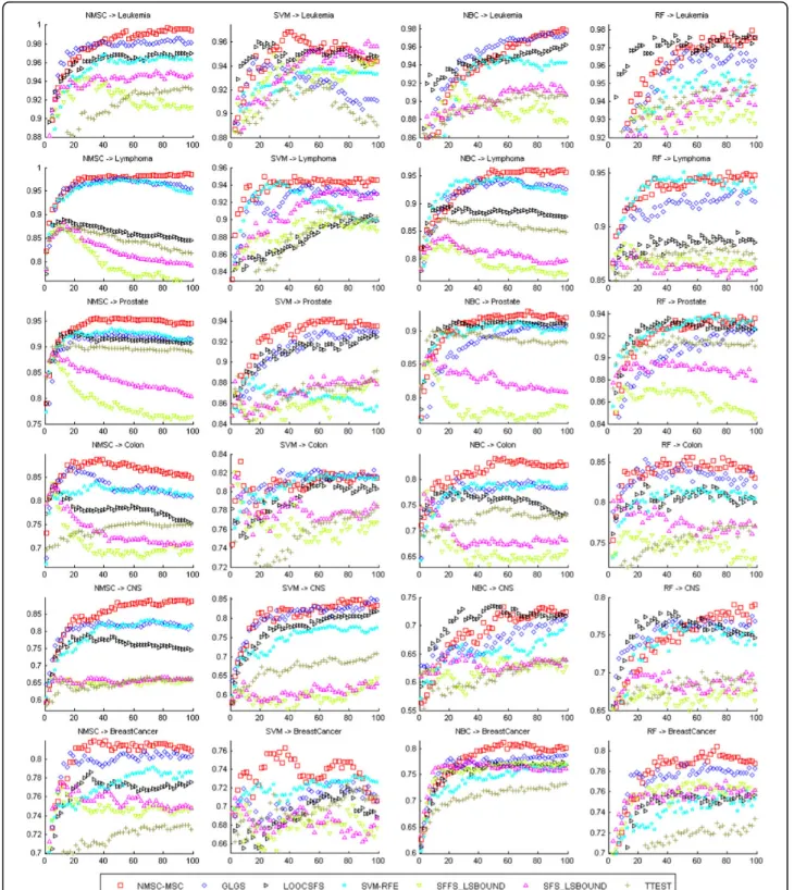
Figure 1 lists the average testing accuracies of the gene selection methods with classifiers NMSC, SVM, NBC, and RF. Again, the performances of NBC-MMC, NMSC-MMC, NBC-MSC, and NMSC-MSC are close to one another; therefore, the average testing accuracies of the gene selection methods NBC-MMC, NMSC-MMC, and NBC-MSC are not listed in the figures. It indicates that the average testing accuracy of NMSC-MSC is the best, followed by GLGS, LOOCSFS, and SVM-RFE. SFS-LS bound, SFFS-SFS-LS bound, and T-TEST did not per-form well. Figure 1 also demonstrates that, spanning several data sets and learning classifiers, the perfor-mance and stabilization of the gene selection method of NMSC-MSC is the best.

Testing results under the best training

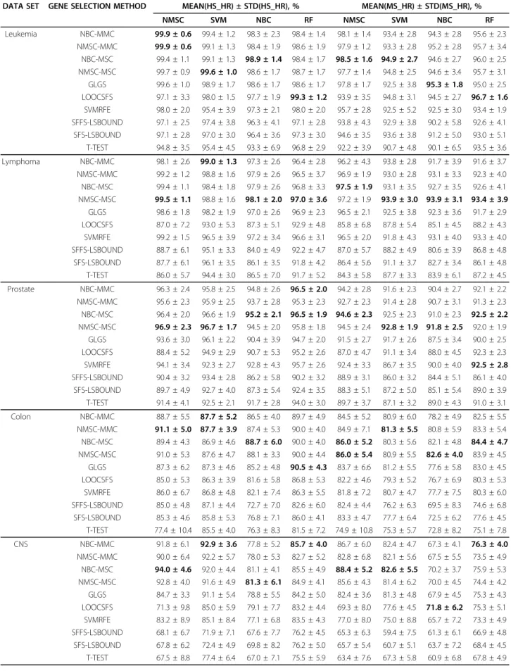
Table 1 provides the mean values and standard errors of the testing accuracies ms_hr(i), (i = 1, 2,..., 20) and the highest testing accuracies hs_hr(i), (i = 1, 2, ..., 20) under the highest training classification, respectively. After applying each classifier to each data set, the high-est mean value of the ten gene selection methods is shaded. In each data set, the highest mean value in the shade is in bold. With the use of the four learning clas-sifiers, under the best training, RFA, GLGS, LOOCSFS, SVMRFE, SFS-LSBOUND, SFFS-LSBOUND, and T-test respectively achieve the highest testing accuracies (HS_HR), 99.9%, 99.6%, 99.3%, 98.0%, 97.4%, 97.3%, and 96.8% for the leukemia data set; 99.5%, 98.6%, 93.0%, 99.2%, 95.1%, 96.1%, and 94.4% for lymphoma; 96.9%, 96.1%, 95.2%, 95.7%, 93.4%, 92.7%, and 94.0% for pros-tate; 91.1%, 90.5%, 86.8%, 86.8%, 87.1%, 86.0%, and 85.5% for colon; 94.0%, 91.1%, 85.0%, 85.1%, 76.2%, 76.2%, and 77.4% for CNS; and 85.9%, 83.7%, 80.3%, 80.4%, 81.5%, 81.3%, and 77.6% for the breast cancer data set. In applying the ten gene selection methods to the six benchmark data sets, all the highest testing accuracies are obtained from the gene set chosen by RFA.

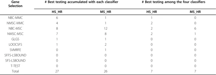
Table 2 lists the number of occurrences for each gene selection method that achieved the best testing accuracy. Table 2 shows that 61 out of 67 highest mean values were obtained by MMC- or MSC-based methods; GLGS, LOOCSFS, and SVMRFE obtained the best twice, three times, and once, respectively; LSBOUND and T-TEST never got the best value. Results indicate that RFA outperforms other gene selection methods.

On the other side, to see whether the new methods are superior to others, regression models were built based on average testing accuracy (ms_hr) and highest testing accuracy (hs_hr), respectively, with data set (six benchmark microarray data set), gene selection method (four new methods and six other methods) and classifier

(four classification methods) as independent variables. After adjusting data set effect and classifier effect, the main effects for the new feature selection methods (NBC-MMC, MMC, NBC-MSC, and NMSC-MSC) and others (GLGS, LOOCSFS, SVMRFE, SFS-LSBOUND, SFFS-SFS-LSBOUND, and T-test) are 91.86%, 91.67%, 92.47%, 92.27%, 90.65%, 86.96%, 88.89%, 84.70%, 85.38%, and 83.93% for the highest testing accuracy, and 86.38%, 86.15%, 87.30%, 86.97%, 85.48%, 82.76%, 83.96%, 79.45%, 80.58%, and 79.36% for the average testing accu-racy, respectively. Table 3 gives the p-values of testing superiority of each new method to other six methods, which are calculated based on one-tailed t-test from the output of the regression models. From the p-values, the performances of our new methods are statistically signif-icantly better than all other methods (most p-values are <0.0001) except for GLGS. From Table 3 MSC-based methods (NBC-MSC, NMSC-MSC) are significantly bet-ter than GLGS based on both highest testing accuracy and average testing accuracy at a significance level of 0.05. Although the p-values for NBC-MMC and NMSC-MMC to GLGS are not small enough due to the small sample size (only six testing data sets) and therefore lower power, we would expect that the differences will be detected at lower significance levels if more data sets are used. To see whether the four new gene methods perform differently, we also test each pair of the four methods and calculate the p-values based on two-tailed t-test from the output of the regression models. All the p-values are bigger than 0.2, so the four new methods perform equally well.

Comparison of LPPO and random strategy

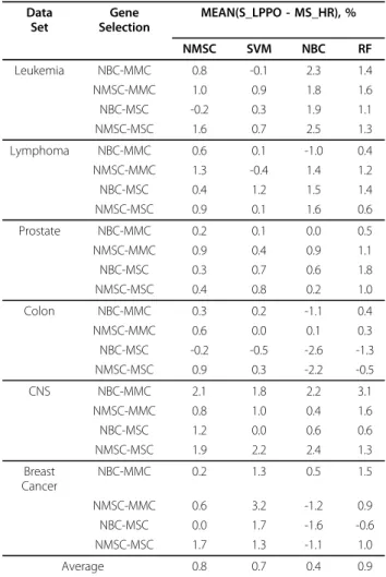
Table 4 lists the mean values of the differences between the testing values (denoted as S_LPPO) by applying NMSC, SVM, NBC, and RF to LPPO and ms_hr. This table shows that, on average, LPPO is superior to the random strategy under the best training accuracies. In summary, spanning the six benchmark data sets, in comparison with ms_hr, LPPO improves the testing accuracy by 0.8% for NMSC, 0.7% for SVM, 0.4% for NBC, and 0.9% for RF on average.

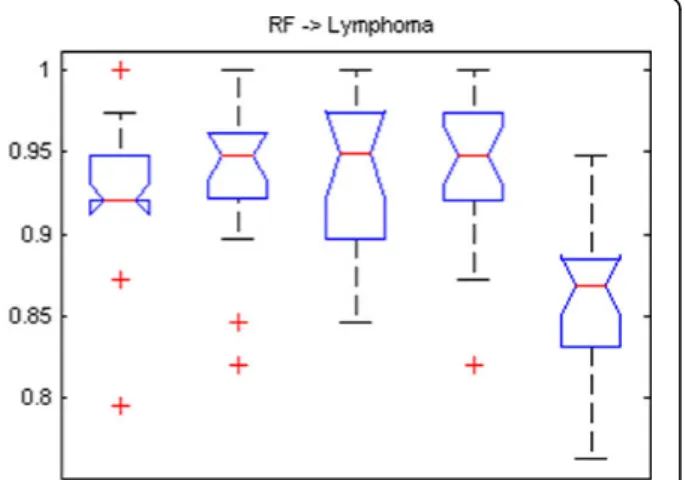
Comparison of LPPO and varSelRF

Figure 2 gives the boxplots of the testing values with the use of learning classifier random forest for the feature sets from LPPO with RFA and varSelRF. The gene selec-tion methods are MMC, NMSC-MMC, NBC-MSC, NMSC-NBC-MSC, and varSelRF from left to right in each subfigure. Figure 2 indicates that the testing accuracies by applying random forest to the feature sets of LPPO with RFA are better than those of varSelRF. In comparison with varSelRF, LPPO with RFA increases the average testing accuracy by about 5% for the

Figure 1The average testing accuracies of different gene selection methods for six benchmark data sets by using the classifiers (NBC, NMSC, SVM, RF). X-axis and y-axis give the feature dimension and testing accuracy values, respectively.

Table 1 Mean values and standard errors of hs_hr and ms_hr.

DATA SET GENE SELECTION METHOD MEAN(HS_HR) ± STD(HS_HR), % MEAN(MS_HR) ± STD(MS_HR), %

NMSC SVM NBC RF NMSC SVM NBC RF Leukemia NBC-MMC 99.9 ± 0.6 99.4 ± 1.2 98.3 ± 2.3 98.4 ± 1.4 98.1 ± 1.4 93.4 ± 2.8 94.3 ± 2.8 95.6 ± 2.3 NMSC-MMC 99.9 ± 0.6 99.1 ± 1.3 98.4 ± 1.9 98.6 ± 1.9 97.9 ± 1.2 93.3 ± 2.8 95.2 ± 2.8 95.7 ± 3.4 NBC-MSC 99.4 ± 1.1 99.1 ± 1.3 98.9 ± 1.4 98.4 ± 1.7 98.5 ± 1.6 94.9 ± 2.7 94.6 ± 2.7 96.0 ± 2.5 NMSC-MSC 99.7 ± 0.9 99.6 ± 1.0 98.6 ± 1.7 98.7 ± 1.7 97.7 ± 1.4 94.8 ± 2.5 94.6 ± 3.4 95.7 ± 3.1 GLGS 99.6 ± 1.0 98.9 ± 1.7 98.6 ± 1.7 98.6 ± 1.7 97.8 ± 1.7 92.5 ± 3.8 95.3 ± 1.8 95.0 ± 2.5 LOOCSFS 97.1 ± 3.3 98.0 ± 1.5 97.7 ± 1.9 99.3 ± 1.2 93.9 ± 3.5 94.8 ± 3.1 94.5 ± 2.7 96.7 ± 1.6 SVMRFE 98.0 ± 2.0 95.4 ± 3.9 97.3 ± 2.1 98.0 ± 2.0 95.7 ± 2.8 92.5 ± 5.2 92.5 ± 3.0 93.4 ± 1.9 SFFS-LSBOUND 97.1 ± 2.5 97.4 ± 3.8 96.3 ± 4.1 97.1 ± 2.8 93.8 ± 4.3 92.9 ± 3.8 90.2 ± 5.8 92.6 ± 4.1 SFS-LSBOUND 97.1 ± 2.8 97.0 ± 3.0 96.4 ± 3.6 97.3 ± 3.0 94.6 ± 3.5 93.6 ± 3.8 91.2 ± 5.0 93.0 ± 5.1 T-TEST 94.8 ± 3.5 95.4 ± 4.5 93.3 ± 6.9 96.8 ± 2.9 92.2 ± 3.9 90.7 ± 4.8 90.1 ± 6.5 93.5 ± 3.6 Lymphoma NBC-MMC 98.1 ± 2.6 99.0 ± 1.3 97.3 ± 2.6 96.4 ± 2.8 96.2 ± 4.3 93.8 ± 2.8 91.7 ± 3.9 91.6 ± 3.7 NMSC-MMC 99.2 ± 1.2 98.8 ± 1.6 97.9 ± 2.6 96.5 ± 3.7 96.9 ± 1.9 93.0 ± 2.8 93.1 ± 3.3 92.3 ± 4.0 NBC-MSC 99.4 ± 1.1 98.4 ± 1.8 97.9 ± 2.6 96.8 ± 3.3 97.5 ± 1.9 93.1 ± 3.5 92.7 ± 3.5 92.6 ± 4.1 NMSC-MSC 99.5 ± 1.1 98.8 ± 1.6 98.1 ± 2.0 97.0 ± 3.6 97.2 ± 1.9 93.9 ± 3.0 93.9 ± 3.1 93.4 ± 3.9 GLGS 98.6 ± 1.8 98.2 ± 1.9 97.0 ± 2.6 96.9 ± 2.3 96.5 ± 2.1 92.5 ± 3.8 92.3 ± 3.6 91.7 ± 2.9 LOOCSFS 87.0 ± 7.2 93.0 ± 5.3 87.3 ± 5.1 92.9 ± 4.8 85.8 ± 6.8 87.8 ± 5.4 85.1 ± 4.5 88.2 ± 4.3 SVMRFE 99.2 ± 1.5 96.5 ± 3.9 97.2 ± 3.4 96.6 ± 3.1 96.5 ± 2.0 91.8 ± 4.3 93.1 ± 4.0 93.3 ± 4.0 SFFS-LSBOUND 88.7 ± 6.1 95.1 ± 3.3 84.0 ± 4.9 92.2 ± 4.7 87.0 ± 5.7 88.2 ± 4.9 80.6 ± 3.9 86.8 ± 4.8 SFS-LSBOUND 87.7 ± 6.1 96.1 ± 3.5 86.1 ± 3.5 91.8 ± 4.2 86.4 ± 5.6 91.1 ± 3.7 82.7 ± 3.4 86.1 ± 4.8 T-TEST 86.0 ± 5.7 94.4 ± 3.0 86.5 ± 7.0 91.7 ± 5.2 84.3 ± 5.8 87.7 ± 3.3 83.9 ± 6.1 87.2 ± 4.5 Prostate NBC-MMC 96.3 ± 2.4 95.8 ± 2.5 94.8 ± 2.6 96.5 ± 2.0 94.2 ± 2.8 91.6 ± 2.3 90.4 ± 2.7 92.1 ± 2.2 NMSC-MMC 95.6 ± 2.3 95.9 ± 2.5 93.7 ± 2.8 95.3 ± 2.3 92.7 ± 2.3 91.4 ± 2.8 90.7 ± 3.1 91.3 ± 2.3 NBC-MSC 96.4 ± 2.0 96.6 ± 1.9 95.2 ± 2.1 96.5 ± 1.9 94.6 ± 2.3 92.5 ± 2.3 91.0 ± 2.3 92.5 ± 2.2 NMSC-MSC 96.9 ± 2.3 96.7 ± 1.7 94.5 ± 2.0 95.8 ± 1.8 94.5 ± 2.4 92.8 ± 1.9 91.8 ± 2.5 92.0 ± 1.9 GLGS 93.6 ± 3.0 96.1 ± 2.2 90.4 ± 3.9 94.7 ± 2.0 91.5 ± 2.7 91.7 ± 2.6 87.5 ± 3.4 90.0 ± 2.5 LOOCSFS 88.4 ± 5.2 94.9 ± 2.9 90.7 ± 5.3 95.2 ± 2.6 87.0 ± 4.7 91.1 ± 3.4 88.0 ± 4.5 92.3 ± 2.3 SVMRFE 94.1 ± 3.4 92.3 ± 2.7 92.8 ± 4.3 95.7 ± 2.6 92.4 ± 3.3 86.7 ± 3.5 90.0 ± 4.0 92.5 ± 2.8 SFFS-LSBOUND 90.4 ± 3.2 93.4 ± 2.8 86.2 ± 5.8 90.2 ± 3.2 88.9 ± 3.1 86.0 ± 3.2 84.4 ± 5.1 86.1 ± 4.0 SFS-LSBOUND 89.7 ± 4.9 92.7 ± 4.0 87.3 ± 5.4 92.4 ± 3.5 88.3 ± 5.1 87.2 ± 5.0 85.1 ± 5.4 89.0 ± 3.9 T-TEST 91.4 ± 4.1 92.5 ± 2.1 91.7 ± 2.8 94.0 ± 3.0 89.7 ± 3.7 87.1 ± 3.2 89.0 ± 4.3 91.0 ± 3.1 Colon NBC-MMC 88.7 ± 5.5 87.7 ± 5.2 86.5 ± 4.0 89.7 ± 4.9 84.5 ± 5.2 80.9 ± 6.0 78.2 ± 4.9 82.5 ± 5.5 NMSC-MMC 91.1 ± 5.0 87.7 ± 3.9 87.4 ± 5.3 90.0 ± 4.0 84.9 ± 7.1 81.3 ± 5.5 80.8 ± 5.9 83.3 ± 5.4 NBC-MSC 89.4 ± 4.3 86.9 ± 4.6 88.7 ± 6.0 90.0 ± 4.0 86.0 ± 5.2 80.3 ± 5.6 82.1 ± 4.8 84.4 ± 4.7 NMSC-MSC 91.0 ± 5.3 87.6 ± 4.7 88.1 ± 3.3 90.0 ± 4.4 86.0 ± 5.4 80.9 ± 5.5 82.6 ± 4.0 83.9 ± 4.5 GLGS 87.3 ± 6.2 87.3 ± 4.6 85.2 ± 4.8 90.5 ± 4.3 83.7 ± 6.6 81.2 ± 5.5 77.6 ± 5.8 83.0 ± 4.5 LOOCSFS 85.0 ± 5.3 86.3 ± 3.9 81.6 ± 5.8 86.8 ± 5.3 82.2 ± 4.6 79.3 ± 5.2 76.7 ± 6.9 80.3 ± 5.3 SVMRFE 86.0 ± 6.7 86.8 ± 4.8 82.1 ± 7.4 86.3 ± 5.5 81.8 ± 7.2 80.7 ± 4.7 77.7 ± 7.5 80.3 ± 6.0 SFFS-LSBOUND 85.0 ± 4.8 87.1 ± 4.4 72.7 ± 7.0 82.6 ± 6.0 82.4 ± 4.4 76.2 ± 6.3 69.5 ± 8.3 74.6 ± 6.8 SFS-LSBOUND 85.3 ± 4.6 85.8 ± 5.3 76.8 ± 7.1 86.0 ± 4.1 83.3 ± 4.7 77.7 ± 6.4 72.5 ± 6.2 77.6 ± 4.5 T-TEST 77.4 ± 10.4 85.5 ± 4.0 76.3 ± 8.3 81.5 ± 7.2 74.9 ± 10.8 75.3 ± 5.7 72.8 ± 8.2 75.1 ± 7.8 CNS NBC-MMC 91.8 ± 6.1 92.9 ± 3.6 77.8 ± 5.2 85.7 ± 4.0 86.7 ± 6.0 82.4 ± 4.7 67.3 ± 4.1 76.3 ± 4.0 NMSC-MMC 90.0 ± 6.4 92.2 ± 5.7 78.0 ± 5.3 82.7 ± 5.2 82.8 ± 6.8 82.1 ± 5.6 67.5 ± 5.5 73.5 ± 4.9 NBC-MSC 94.0 ± 4.6 92.0 ± 4.4 81.1 ± 4.1 85.5 ± 4.9 88.4 ± 5.2 82.6 ± 5.5 70.2 ± 3.7 75.9 ± 5.3 NMSC-MSC 92.8 ± 4.0 91.6 ± 4.9 81.3 ± 6.1 84.9 ± 4.1 85.6 ± 4.3 81.4 ± 6.2 70.0 ± 4.5 74.4 ± 4.2 GLGS 84.7 ± 3.3 91.1 ± 5.4 78.8 ± 5.5 84.2 ± 5.0 82.4 ± 3.6 81.3 ± 4.8 67.9 ± 4.5 75.3 ± 4.3 LOOCSFS 71.3 ± 9.8 85.0 ± 5.9 79.1 ± 7.7 83.2 ± 4.4 69.3 ± 8.0 77.6 ± 4.5 71.8 ± 6.2 75.3 ± 5.1 SVMRFE 83.2 ± 8.9 85.1 ± 8.4 77.1 ± 6.8 83.5 ± 4.3 77.0 ± 8.0 75.0 ± 8.8 65.7 ± 7.2 73.3 ± 4.9 SFFS-LSBOUND 68.1 ± 6.7 71.9 ± 7.1 67.6 ± 7.7 76.2 ± 4.5 65.3 ± 6.3 59.4 ± 7.5 61.3 ± 6.1 66.9 ± 4.8 SFS-LSBOUND 67.8 ± 6.2 72.4 ± 4.9 69.8 ± 8.2 76.2 ± 5.0 65.7 ± 5.4 60.7 ± 5.1 63.7 ± 7.2 68.4 ± 4.5 T-TEST 67.5 ± 8.8 77.4 ± 6.4 67.0 ± 7.1 75.5 ± 5.9 63.4 ± 7.6 67.3 ± 5.8 60.9 ± 6.8 67.8 ± 4.9

leukemia data set, 9% for lymphoma, 3% for colon and prostate, 10% for CNS, and 14% for the breast cancer data set.

Computational efficiency

In microarray data analysis, generally, the number of features in the final feature set is far smaller than the total variables. Suppose the number of total variables is n, the number of features of the final feature set is m (m <<n). In forward feature selection, with the use of some learning classifier, the computational time isF(s, d) for as×dfeature matrix, heresis the number of data samples (s << n) andd is the feature dimensionality at each sample. Without losing the generality, ifd1<d2,F(s, d1) <F(s, d2). The computational cost of our feature selection algorithm is analyzed as follows.

Let T1denote the total computational time for super-vised learning T1= n∗F(s, 1) +(n−1)∗F(s, 2) + . . . + (n−m+ 1)∗F(s,m) ≤n+ (n−1) + ... + (n−m+ 1)∗F(s,m) =m∗(2∗n−m+ 1) 2 ∗F(s,m) (4)

Let T2 denote the computational time for similarity calculation among the candidates and chosen genes, the calculation time between two single- variant vectors with s samples is C(s), then

T2≤(n−1)∗C(s) + 2∗(n−2)∗C(s) + ... +m∗(n−m)∗C(s) =C(s)∗ 1 2nm(m+ 1)− m i=1 i2 (5)

Due to the fact of m << n and s << n with microarray data, the computational cost of our feature selection is obtained by

T=T1+T2∼O(n) (6)

Conclusions

Our study shows that our gene selection method Recur-sive Feature Addition (RFA) obtained the best classifica-tion performance in the comparison. RFA utilizes supervised learning to obtain the best classification, and indentifies the subsequent gene recursively based on the similarity measures between the chosen gene set and the candidates to minimize the redundancy of the genes

Table 2 The number of occurrences of the best testing in Table 1

Gene Selection

# Best testing accumulated with each classifier # Best testing among the four classifiers

HS_HR MS_HR HS_HR MS_HR NBC-MMC 6 1 1 0 NMSC-MMC 4 1 2 0 NBC-MSC 8 12 2 6 NMSC-MSC 7 8 2 1 GLGS 1 1 0 0 LOOCSFS 1 2 0 0 SVMRFE 0 1 0 0 SFFS-LSBOUND 0 0 0 0 SFS-LSBOUND 0 0 0 0 T-TEST 0 0 0 0 Total 27 26 7 7

Table 1 Mean values and standard errors of hs_hr and ms_hr.(Continued)

Breast NBC-MMC 82.5 ± 6.0 82.9 ± 3.5 84.1 ± 3.0 84.1 ± 3.6 81.3 ± 5.7 73.2 ± 3.8 78.4 ± 3.4 78.4 ± 3.8 NMSC-MMC 83.9 ± 4.6 82.0 ± 3.3 82.4 ± 4.3 83.7 ± 4.7 80.4 ± 4.0 72.0 ± 3.8 78.4 ± 4.3 77.0 ± 4.3 NBC-MSC 83.4 ± 5.8 83.5 ± 3.8 85.8 ± 3.1 85.9 ± 4.7 81.5 ± 5.3 74.9 ± 3.3 79.1 ± 3.0 79.4 ± 4.1 NMSC-MSC 82.8 ± 4.4 82.4 ± 3.8 84.1 ± 4.0 83.9 ± 4.0 79.6 ± 4.0 73.7 ± 3.9 79.2 ± 3.8 77.7 ± 4.0 GLGS 80.8 ± 3.7 79.3 ± 4.5 81.4 ± 4.1 83.7 ± 4.6 79.2 ± 3.9 70.7 ± 4.6 77.8 ± 3.7 77.0 ± 4.2 LOOCSFS 71.7 ± 6.5 77.3 ± 5.2 78.0 ± 5.8 80.3 ± 3.8 70.4 ± 6.5 69.2 ± 4.7 74.7 ± 5.1 74.3 ± 4.2 SVMRFE 74.3 ± 7.1 78.3 ± 5.2 77.2 ± 5.3 80.4 ± 4.1 73.2 ± 6.6 72.1 ± 5.8 73.9 ± 4.5 73.9 ± 3.7 SFFS-LSBOUND 76.2 ± 5.2 78.9 ± 2.8 76.9 ± 7.3 81.5 ± 5.3 75.0 ± 5.3 67.8 ± 3.3 75.2 ± 6.8 75.6 ± 4.9 SFS-LSBOUND 77.5 ± 5.6 78.9 ± 4.2 79.8 ± 5.2 81.3 ± 5.2 75.8 ± 5.5 68.0 ± 4.7 76.9 ± 6.3 75.4 ± 5.2 T-TEST 71.1 ± 5.3 77.6 ± 5.2 72.6 ± 6.3 76.3 ± 5.7 69.3 ± 5.3 69.9 ± 3.6 70.5 ± 5.8 71.1 ± 5.8 In each data set, the highest mean value is highlighted in bold

within the selected subset; hence it obtains more infor-mative and differently expressed genes. Based on RFA, we also propose an algorithm, Lagging Prediction Peep-hole Optimization (LPPO), to determine the optimal feature set. Using six popular benchmark data sets, we compared RFA with other gene selection methods. Our studies showed that RFA outperformed other methods with the use of the four popular classifiers: NMSC, NBC, SVM, and random forest. Results also showed that, on average, LPPO is superior to a random strategy

under the best training and that it outperformed the random forest based gene selection method varSelRF.

Methods

Supervised recursive learning

Our method of RFA uses supervised learning to achieve the highest level of training accuracy and statistical simi-larity measures to choose the next variable with the least dependence on or correlation to the already identified variables as follows:

1. Insignificant genes are removed according to their statistical insignificance. Specifically, a gene with a high p-value is usually not differently expressed and therefore has little contribution in distinguishing normal tissues from tumor tissues or in classifying different types of tissues. To reduce the computational load, those genes should be removed. The filtered gene data is then nor-malized. Here we use the standard normalization method, MANORM, which is available from MATLAB bioinformatics toolbox.

2. Each individual gene is selected by supervised learn-ing. A gene with highest classification accuracy is cho-sen as the most important feature and the first element of the feature set. If multiple genes achieve the same highest classification accuracy, the one with the lowest p-value measured by test-statistics (e.g., score test), is the target of the first element. At this point the chosen feature set, G1, contains just one element, g1, corre-sponding to the feature dimension one.

3. The (N+1)stdimension feature set,GN+1= {g1,g2, ..., gN,gN+1} is obtained by addinggN+1to the Nth dimen-sion feature set,GN = {g1, g2, ...,gN}. The choice ofgN+1 is described as follows:

Add each gene gi (gi ∉ GN) into GN and obtain the classification accuracy of the feature setGN∪{gi}. The gi (gi ∉ GN) associated with the group, GN ∪{gi} that obtains the highest classification accuracy, is the candi-date forgN+1(not yetgN+1). Considering the large num-ber of variables, it is highly possible that multiple features correspond to the same highest classification accuracy. These multiple candidates are placed into the set C, but only one candidate from Cwill be identified asgN+1. How to make the selection is described next. Table 4 Comparison of LPPO and Random Strategy

Data Set Gene Selection MEAN(S_LPPO - MS_HR), % NMSC SVM NBC RF Leukemia NBC-MMC 0.8 -0.1 2.3 1.4 NMSC-MMC 1.0 0.9 1.8 1.6 NBC-MSC -0.2 0.3 1.9 1.1 NMSC-MSC 1.6 0.7 2.5 1.3 Lymphoma NBC-MMC 0.6 0.1 -1.0 0.4 NMSC-MMC 1.3 -0.4 1.4 1.2 NBC-MSC 0.4 1.2 1.5 1.4 NMSC-MSC 0.9 0.1 1.6 0.6 Prostate NBC-MMC 0.2 0.1 0.0 0.5 NMSC-MMC 0.9 0.4 0.9 1.1 NBC-MSC 0.3 0.7 0.6 1.8 NMSC-MSC 0.4 0.8 0.2 1.0 Colon NBC-MMC 0.3 0.2 -1.1 0.4 NMSC-MMC 0.6 0.0 0.1 0.3 NBC-MSC -0.2 -0.5 -2.6 -1.3 NMSC-MSC 0.9 0.3 -2.2 -0.5 CNS NBC-MMC 2.1 1.8 2.2 3.1 NMSC-MMC 0.8 1.0 0.4 1.6 NBC-MSC 1.2 0.0 0.6 0.6 NMSC-MSC 1.9 2.2 2.4 1.3 Breast Cancer NBC-MMC 0.2 1.3 0.5 1.5 NMSC-MMC 0.6 3.2 -1.2 0.9 NBC-MSC 0.0 1.7 -1.6 -0.6 NMSC-MSC 1.7 1.3 -1.1 1.0 Average 0.8 0.7 0.4 0.9

Table 3 P-values from testing superiority of new methods to others

Method NBC-MMC NMSC-MMC NBC-MSC NMSC-MSC HS_HR MS_HR HS_HR MS_HR HS_HR MS_HR HS_HR MS_HR GLGS 0.092 0.15 0.13 0.22 0.023 0.0212 0.038 0.048 LOOCSFS <0.0001 <0.0001 <0.0001 0.0001 <0.0001 <0.0001 <0.0001 <0.0001 SVMRFE <0.0001 <0.0001 <0.0001 0.0077 <0.0001 0.0001 <0.0001 0.0004 SFFS-LSBOUND <0.0001 <0.0001 <0.0001 <0.0001 <0.0001 <0.0001 <0.0001 <0.0001 SFS-LSBOUND <0.0001 <0.0001 <0.0001 <0.0001 <0.0001 <0.0001 <0.0001 <0.0001 T-TEST <0.0001 <0.0001 <0.0001 <0.0001 <0.0001 <0.0001 <0.0001 <0.0001

Figure 2Boxplots of testing accuracies of the LPPO with four gene selection methods using two different classifiers (NBC, NMSC) compared to varSelRF for six data sets. RF is the final classifier. All six data sets demonstrate that varSelRF accuracies are lower than our proposed feature selection and optimization algorithm with the same RF classifier.

Candidate feature addition

To find the most informative (or least redundant) next featuregN+1, two formulas may be designed by measur-ing the statistical similarity between the chosen feature set and each candidate. Here we use, say, Pearson’s cor-relation coefficient [28] between chosen features gn (gn

ÎGN, n =1, 2,..., N) and candidategc (gcÎC) to mea-sure the similarity.

In the first formula, the sum of the square of the cor-relation, SC, is calculated to measure the similarity and is defined as follows: SCgc = N n=1 cor2gc, gn n= 1, 2 ...N (7) Where,gc ÎC, gnÎ GN.

Then selection ofgN+1 can be based on the Minimum Sum of the square of the Correlation (MSC), that is,

gN+1← {gc|SC(gc) = min(SC).gc∈C} (8) In the second formula, the maximum value of the square of the correlation, MC, is calculated:

MC(gc) = max(cor2(gc,gn)), n= 1, 2, ...,N (9) Where,gc ÎC, gnÎ GN.

The selection of gN+1 follows the criterion that the MC value is the minimum, which we call Minimum of Maximum value of the square of the Correlation (MMC).

gN+1← {gc|MC(gc) = min(MC).gc∈C} (10) In the methods mentioned above, a feature is recur-sively added to the chosen feature set based on super-vised learning and the similarity measures. With the use of a classifier XXX, we call the first gene selection method XXX-MSC and the second one XXX-MMC. For example, if the classifier is Naive Bayes Classifier (NBC), we call the two strategies NBC-MSC and NBC-MMC, respectively.

Lagging Prediction Peephole Optimization (LPPO)

We want to find a combination of features (genes) that yields the best performance on breaking down solvents. Normally, with the recursive addition for the next fea-ture, the training accuracy will increase and reach a peak classification performance at some point, and then may maintain it with subsequent feature additions; but after that the training accuracy may decrease. Generally speaking, all strategies for determining the final feature set should be based on the best training classification. In high-volume data analysis, it is common that the best training accuracy corresponds to different feature sets; that is, multiple feature sets achieve the same highest

training accuracy. However, although all these feature sets are associated with the same highest training accu-racy, the testing accuracy of these feature sets may be different. Among these highest training feature sets, the one having the best testing accuracy is called the opti-mal feature set, which is highly complicated to charac-terize when a sample size is small. Either applying different gene methods to the same training samples, or applying the same gene selection method to different training samples, or applying different learning classifiers to the same training samples, will produce a different optimization of the feature set. Pochet et al.[29] pre-sented a method of determining the optimal number of genes by means of a cross-validation procedure; the drawback of this method is that it actually utilizes whole data information, including training samples and testing samples.

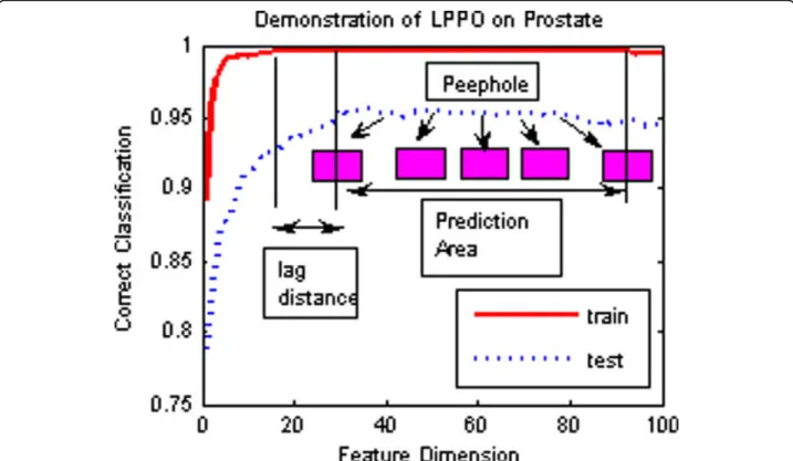
How do we choose the optimal feature set? If there are multiple best training classifications, a random choice, called random strategy, works for best training classification. In the recursive addition of the features, for training samples, a classification model is one of the best methods. But for testing samples, at this point, the classification model may not be optimal because of the difference between the training samples and the testing samples; the optimal classification model will lag in appearance (see Figure 1). Based on this observation, we propose the following algorithm for optimization.

Under feature dimensionj, the training accuracy of theithexperiment is r(i, j). If the feature set Gk, corre-sponding to feature dimension k, has the best training accuracy in the trainings from the feature setG1 to GD, corresponding to the feature dimensions from 1 to D, letHR denote the set that contains all the combinations of Gk, corresponding to all the feature set having the highest classification accuracy under feature dimension 1 to D.

HR={Gk|r(i,k) = max(r(i,•)), 1≤k≤D} (11) In general, the best classification model for testing samples will lag in appearance behind the initial best training model. We will exclude the elements of HR that correspond to the initial best training. The remain-ing elements in HRconstitute the candidate set HRC for optimization.

Each element in HRC is associated with the best training accuracy. We set a peephole for each element and choose the element associated with the optimal peephole. The details are described as follows:

a. For each elementGkÎHRC, the peephole over Gk with length of 2l+1 covers the feature sets Gk-l, Gk-l+1, ..., Gk , ..., Gk+l-1, Gk+l, corresponding to the training accuracyr(i, k-l),r(i, k-l+1), ...,r(i, k), ...,r(i, k+l-1), r(i, k

+l). The mean training value of the peephole is denoted by mp_r(i, k).

mp r(i,k) = (1/(2l+ 1))m=k+l

m=k−lr(i,m) (12) The peephole with the best classification of mp_r is then chosen as the optimal one.

b. If there are multiple optimal peepholes, then we apply random forest to these peepholes and check the mean values of the Out-of-Bag (OOB) error rates [24,25,30]. The feature setsGk-l,Gk-l+1, ..., Gk,, ..., Gk+l-1, Gk+lcorrespond to the OOB errors, oob_e(i,k-l), oob_e (i,k-l+1), ..., oob_e(i,k), ..., oob_e(i,k+l-1), oob_e(i,k+l). The mean value of the OOB errors is denoted by mp_oob_e(i,k)

mp oob e(i,k) = (1/(2l+ 1))m=k+l

m=k−loob e(i,m) (13) The peephole with minimum mp_oob_e is the optimal one.

c. If there are multiple peepholes corresponding to the best mp_r and minimum mp_oob_e, then setl+1 ®l, and repeat ‘a’to‘c’, until a unique optimal peephole is determined.

d. The feature set located at the center of the final optimal peephole is chosen as the final optimal feature set.

This optimization of RFA is called Lagging Prediction Peephole Optimization (LPPO). Figure 3 briefly outlines the LPPO on the prostate data set, which was studied by Singhet al. [31].

Data sets

The following six benchmark microarray data sets have been extensively studied and used in our experiments to compare the performances of our methods with others. Data sources that are not specified are available at: http://www.broad.mit.edu/cgi-bin/cancer/datasets.cgi.

1) The LEUKEMIA data set consists of two types of acute leukemia: 48 acute lymphoblastic leukemia (ALL) samples and 25 acute myeloblastic leukemia (AML) samples with over 7129 probes from 6817 human genes. It was studied by Golubet al.[32].

2) The LYMPHOMA data set consists of 58 diffuse large B-cell lymphoma (DLBCL) samples and 19 follicu-lar lymphoma (FL) samples. It was studied by Shipp et al. [33]. The data file, lymphoma_8_lbc_fscc2_rn.res, and the class label file, lymphoma_8_lbc_fscc2.cls were used in our experiments for identifying DLBCL and FL.

3) The PROSTATE data set used by Singhet al.[31] contains 52 prostate tumor samples and 50 non-tumor prostate samples.

4) The COLON cancer data set used by Alon et al. [34] contains 62 samples collected from colon-cancer

patients. Among them, 40 tumor biopsies are from tumors, and 22 normal biopsies are from healthy parts of the colons of the same patients. Based on the confi-dence in the measured expression levels, 2000 genes were selected. The data source is available at: http:// microarray.princeton.edu/oncology/affydata/index.html.

5) The Central Nervous System (CNS) embryonal tumor data set that was originally studied by Pomeroy et al.[35] contains 60 patient samples. Among them, 21 are survivors who are alive after treatment, and 39 are failures who succumbed to their diseases. There are 7129 genes.

6) The Breast cancer data set studied by Van et al. [36] contains 97 patient samples, 46 of which are relapse patients who had developed distance metastases within 5 years, and 51 patients who are non-relapsed who remained healthy for at least 5 years from the distance after their initial diagnosis. This data source is available at: http://www.rii.com/publications/2002/vantveer.htm.

Experiments

Our experiments are designed as follows:

1. The data sets are first divided randomly into train-ing samples and testtrain-ing samples. The ratio of traintrain-ing samples to testing samples is approximately 1:1 in each class.

2. Recursive feature additions with Naive Bayes Classi-fier (NBC) and Nearest Mean Scaled ClassiClassi-fier (NMSC) for gene selection (NBC-MSC, NBC-MMC, NMSC-MSC, and NMSC-MMC) were applied to the training samples for gene selection. Different feature sets of the gene expression data are produced under feature dimen-sions 1 to 100. We compared the above proposed meth-ods to several recently developed and published gene selection methods: LOOCSFS, GLGS, SVMRFE, SFFS-LS bound, SFS-SFFS-LS bound, and also T-TEST.

3. To compare different gene selection methods, the learning classifiers including NBC, NMSC, SVM [37,38], and Random Forest are applied to the testing samples.

4. The experiments were performed in 20 runs, and the average testing accuracies were compared to evalu-ate performance.

Acknowledgements

The authors are grateful to Matteo Masotti, E Ke Tang, and Xin Zhou for offering their codes of RfeRank, GLGS, LOOCSFS, SFS-LSbound, and SFFS-LSbound, to Ramon Diaz-Uriarte for the help with the use of varSelRF R package. Partial support for this study from the Institute for Complex Additive Systems Analysis, a division of New Mexico Tech, and from Sam Houston State University, is greatly acknowledged.

Author details

1_{Department of Computer Science, Sam Houston State University, Huntsville,}

TX 77341, USA.2Department of Computer Science and Institute of Complex Additive Systems Analysis, New Mexico Institute of Mining and Technology, Socorro, NM 87801, USA.3Biostatistics Epidemiology Research Design Core,

Center for Clinical and Translational Sciences, The University of Texas Health Science Center at Houston, Houston, TX 77030, USA.4_{The Chem21 Group,}

Inc, 1780 Wilson Drive, Lake Forest, IL 60045, USA.5Mathematics and Computer Science, Dept. of Mathematics & Computer Science, South Dakota School of Mines & Technology, Rapid City, SD 57701-3995.6Wuhan University of Science and Technology, Wuhan, Hubei 430081, China.

7

Conjugate and Medicinal Chemistry Laboratory, Division of Nuclear Medicine and Molecular Imaging, Department of Radiology, Brigham and Women’s Hospital and Harvard Medical School, Boston, MA 02115, USA.

8_{Cancer Bioinformatics, Rush University Cancer Center, and Department of}

Internal Medicine, Rush University Medical Center, Chicago, IL 60612, USA.

Authors_’contributions

QL designed the algorithms, performed the study, and wrote the draft; AHS supervised the study and revised the draft; ZC helped designing the algorithms and experiments, provided the statistical analysis, and co-drafted the manuscript; LC, JL, MQ, YP, ZW and HX participated in algorithm design, programming, and helped editing the draft; and YP coordinated the project and assisted the draft and data analyses

Competing interests

The authors do not claim any confliction of interests.

Published: 23 December 2011

References

1. Chen Z, McGee M, Liu Q, Scheuermann RH:A distribution free summarization method for Affymetrix GeneChip Arrays.Bioinformatics

2007,23(3):321-327.

2. Quackenbush J:Computational analysis of microarray data.Nat Rev Genet

2001,2(6):418-427.

3. Hand DJ, Heard NA:Finding groups in gene expression data.J Biomed Biotechnol2005, ,2:215-225.

4. Segal E, Friedman N, Kaminski N, Regev A, Koller D:From signatures to models: understanding cancer using microarrays.Nat Genet2005,

37(Suppl):S38-45.

5. Torrente A, Kapushesky M, Brazma A:A new algorithm for comparing and visualizing relationships between hierarchical and flat gene expression data clusterings.Bioinformatics2005,21(21):3993-3999.

6. Qin Z:Clustering microarray gene expression data using weighted Chinese restaurant process.Bioinformatics2006,22(16):1988-1997. 7. Brazma A, Krestyaninova M, Sarkans U:Standards for system biology.Nat

Rev Genet2006,7:593-605.

8. Newton MA, Kendziorski CM, Richmond CS, Blattner FR, Tsui KW:On differential variability of expression ratios: improving statistical inference about gene expression changes from microarray data.J Comput Biol

2001,8(1):37-52.

9. Long A, Mangalam H, Chan B, Tolleri L, Hatfield G, Baldi P:Improved statistical inference from DNA microarray data using analysis of variance and a Bayesian statistical framework.J Biol Chem276(23):19937-19944. 10. Bo T, Jonassen I:New feature subset selection procedures for

classification of expression profiles.Genome Biol2002,3(4):research0017. 11. Yu J, Chen X-W:Bayesian neural network approaches to ovarian cancer

identification from high-resolution mass spectrometry data.

Bioinformatics2005,21(suppl 1):i487-i494.

12. Pavlidis P, Noble WS:Analysis of strain and regional variation in gene expression in mouse brain.Genome Biol2001,2(10):0042.1-0042.15. 13. Inza I, Sierra B, Blanco R, Larranaga P:Gene selection by sequential search

wrapper approaches in microarray cancer class prediction.Journal of Intelligent and Fuzzy Systems2002,12(1):25-33.

14. Guyon I, Weston J, Barnhill S, Vapnik VN:Gene selection for cancer classification using support vector machines.Machine Learning2002,

46(19):389-422.

15. Liu Q, Sung AH, Chen Z, Xu J:Feature mining and pattern classification for steganalysis of LSB matching steganography in grayscale images.

Pattern Recognition2008,41(1):56-66.

16. Liu Q, Sung AH, Qiao M, Chen Z, Ribeiro B:An improved approach to steganalysis of JPEG images.Information Sciences2010,180(9):1643-1655. 17. Monari G, Dreyfus G:Withdrawing an example from the training set: an analytic estimation of its effect on a nonlinear parameterized model.

18. Rivals I, Personnaz L:MLPs (Mono-Layer Polynomials and Multi-Layer Perceptrons) for nonlinear modeling.Journal of Machine Learning Research

2003,3:1383-1398.

19. Tibshirani R:Regression shrinkage and selection via the lasso.J Royal Statist Soc B1996,58(1):267-288.

20. Tibshirani R:The lasso method for variable selection in the Cox model.

Stat Med1997,16(4):385-395.

21. Krishnapuram B, Carin L, Figueiredo M, Hartemink A:Sparse multinomial logistic regression: fast algorithms, and generalization bounds.IEEE Trans Pattern Anal Mach Intell2005,27(6):957-968.

22. Zhou X, Mao K-Z:LS bound based gene selection for DNA microarray data.Bioinformatics2005,21(8):1559-1564.

23. Tang E-K, Suganthan PN, Yao X:Gene selection algorithms for microarray data based on least square support vector machine.BMC Bioinformatics

2006,7:95.

24. Diaz-Uriarte R, de Andres SA:Gene selection and classification of microarray data using random forest.BMC Bioinformatics2006,7:3. 25. Breiman L:Random forests.Machine Learning2001,45(1):5-32. 26. Guyon I, Elisseeff A:An introduction to variable and feature selection.

Journal of Machine Learning Research2003,3:1157-1182.

27. Liu Q, Sung AH, Chen Z, Liu J, Huang X, Deng Y:Feature selection and classification of MAQC-II breast cancer and multiple myeloma microarray gene expression data.PLoS One2009,4(12):e8250.

28. Tan P, Steinbach M, Kumar V:Introduction to Data MiningAddison-Wesley; 2005, 76-79.

29. Pochet N, De Smet F, Suykens J, De Moor B:Systematic benchmarking of microarray data classification: assessing the role of non-linearity and dimensionality reduction.Bioinformatics2004,20(17):3185-3195. 30. Liaw A, Wiener M:Classification and regression by random forest.R News

2(3):18-22.

31. Singh D,et al:Gene expression correlates of clinical prostate cancer behavior.Cancer Cell2002,1(2):227-235.

32. Golub T,et al:Molecular classification of cancer: class discovery and class prediction by gene expression.Science1999,286(5439):531-537. 33. Shipp M,et al:Diffuse large B-cell lymphoma outcome prediction by

gene expression profiling and supervised machine learning.Nat Med

2002,8(1):68-74.

34. Alon U,et al:Broad patterns of gene expression revealed by clustering analysis of tumor and normal colon tissues probed by oligonucleotide arrays.Proc Natl Acad Sci USA1999,96(12):6745-6750.

35. Pomeroy SL,et al:Prediction of central nervous system embryonal tumor outcome based on gene expression.Nature2002,415:436-442. 36. Van LJ,et al:Gene expression profiling predicts clinical outcome of

breast cancer.Nature2002,415:530-536.

37. Vapnik V:Statistical Learning TheoryJohn Wiley; 1998, ISBN-10: 0471030031. 38. Heijden F, Duin R, Ridder D, Tax D:Classification, Parameter Estimation and

State EstimationJohn Wiley; 2004, ISBN-10: 0470090138.

doi:10.1186/1471-2164-12-S5-S1

Cite this article as:Liuet al.:Gene selection and classification for cancer microarray data based on machine learning and similarity measures.

BMC Genomics201112(Suppl 5):S1.

Submit your next manuscript to BioMed Central and take full advantage of:

• Convenient online submission • Thorough peer review

• No space constraints or color figure charges • Immediate publication on acceptance

• Inclusion in PubMed, CAS, Scopus and Google Scholar • Research which is freely available for redistribution

Submit your manuscript at www.biomedcentral.com/submit