Improving a Particle Swarm Optimization-based Clustering Method

(1)

University of New Orleans University of New Orleans

ScholarWorks@UNO

University of New Orleans Theses and

Dissertations Dissertations and Theses

Spring 5-19-2017

Improving a Particle Swarm Optimization-based Clustering

Method

Sharif Shahadat

University of New Orleans, [email protected]

Follow this and additional works at: https://scholarworks.uno.edu/td

Part of the Other Computer Engineering Commons, and the Other Electrical and Computer Engineering Commons

Recommended Citation Recommended Citation

Shahadat, Sharif, "Improving a Particle Swarm Optimization-based Clustering Method" (2017). University of New Orleans Theses and Dissertations. 2357.

https://scholarworks.uno.edu/td/2357

This Thesis is protected by copyright and/or related rights. It has been brought to you by ScholarWorks@UNO with permission from the rights-holder(s). You are free to use this Thesis in any way that is permitted by the copyright and related rights legislation that applies to your use. For other uses you need to obtain permission from the rights-holder(s) directly, unless additional rights are indicated by a Creative Commons license in the record and/or on the work itself.

(2)

Improving a Particle Swarm Optimization-based Clustering Method

A thesis

Submitted to the Graduate Faculty of the University of New Orleans

in partial fulfillment of the requirements of the degree of

Master of Science in Engineering Electrical By Sharif Shahadat

(3)

Dedication

I am grateful to the Almighty creator for the infinite blessings in my life, which led to the completion of my Master’s thesis. I dedicate this work to my loving parents and my beloved brother, whose prayers and guidance helped me get through this journey. It was due their constant support that made me reach the destination for this journey.

(4)

Acknowledgements

I would like to express heartfelt gratitude to my academic and research advisor, Dr. Dimitrios Charalampidis, for his guidance and constant support that provided the base for this work. I am indebted to him for his patience to go through my thesis repeatedly. His encouraging words gave me confidence when I was struggling through my time in the Master’s Program. The depth of knowledge and his ever-welcoming character have been a great inspiration throughout this journey.

I would like to thank Dr. Vesselin Jilkov, and Dr. Ebrahim Amiri, for accepting the request to serve as members in my thesis committee. Their sincere advices help shape the thesis in the best way possible. I would also like to thank my friends and colleagues, especially Monir Hossain and Sumaiya Iqbal for their invaluable support throughout my studies.

I would like to thank my parents and my brother for their guidance throughout my life. Words are not capable of conveying my feelings towards them.

Finally, I would like to express my deepest gratitude to the University of New Orleans for providing the necessary tools and environment for this work. I recognize that this research would not have been possible without the resources made available by the University.

(5)

List of Tables

3.1 Datasets used for evaluation . . . 26

3.2 Results for Ruspini dataset for the ADPSO algorithm . . . 28

3.3 Results for Ruspini dataset for the DCPSO algorithm . . . 28

3.4 Results for Artificial dataset for the ADCPSO algorithm . . . 28

3.5 Results for Artificial dataset for the DCPSO algorithm . . . 28

3.6 Results for Iris dataset for the ADCPSO algorithm . . . 28

3.7 Results for Iris dataset for the DCPSO algorithm . . . 29

3.8 Results for Automotive dataset for the ADCPSO algorithm. . . 29

3.9 Results for Automotive dataset for the DCPSO algorithm . . . 29

3.10 Results for Sonar dataset for the ADCPSO algorithm . . . 29

3.11 Results for Sonar dataset for the DCPSO algorithm . . . 29

3.12 ADCPSO run time . . . 30

3.13 DCPSO run time . . . 30

3.14 ADCPSO average number of iterations for convergence . . . 30

3.15 ADCPSO average number of iterations for convergence . . . 30

3.16 Improvement achieved by ADCPSO against DCPSO (%) . . . 30

3.17 Best cost achieved by Improved ADCPSO . . . 31

3.18 Execution time for IADCPSO . . . 32

(8)

List of Figures

1.1 Complexity of clustering . . . 3 1.2 Taxonomy of clustering methods . . . 4 1.3 Partitions returned by k-means for non-spherical data . . . 6 3.1 (a) Sample positions of global best and particle, (b) Particle movement

(9)

Abstract

This thesis discusses clustering related works with emphasis on Particle Swarm Optimization (PSO) principles. Specifically, we review in detail the PSO clustering algorithm proposed by Van Der Merwe & Engelbrecht, the particle swarm clustering (PSC) algorithm proposed by Cohen & de Castro, Szabo’s modified PSC (mPSC), and Georgieva & Engelbrecht’s Cooperative-Multi-Population PSO (CMPSO). In this thesis, an improvement over Van Der Merwe & Engelbrecht’s PSO clustering has been proposed and tested for standard datasets. The improvements observed in those experiments vary from slight to moderate, both in terms of minimizing the cost function, and in terms of run time.

(10)

Chapter 1

Introduction

1.1 Motivation

Large datasets are getting more common in the recent years. As a result, it is becoming exceedingly difficult for human analysts to interpret the patterns in large datasets. Cluster analysis or data clustering come to rescue in this regard by offering a large number of vital techniques for the field of pattern recognition. The objective of data clustering is to divide a large amount of data into groups (clusters) based on certain similarity criteria. Clustering finds applications in many fields, including data mining, decision making, bioinformatics, machine learning, object recognition, signal processing, and image segmentation [1–3]. This thesis introduces a novel data clustering algorithm based on Particle Swarm Optimization (PSO).

1.2 Background

Everitt (1974) collected the following two definitions of a cluster [4]:

(11)

“Clusters may be described as connected regions of a multi-dimensional space containing a relatively high density of points, separated from other such regions by a region containing a relatively low density of points.”

Clustering can help discover inherent structures in unlabeled data. Clustering algorithms attempt to group data and reveal these structures by optimizing a certain objective function. Nevertheless, a global optimal solution to a problem might not be always found. Moreover, because of the unsupervised nature of clustering algorithms, it is not always guaranteed that the choice of the objective function is appropriate for the problem at hand. For dimensions higher than three, the solutions found from clustering may often be far away from the optimal solution.

1.3 Complexity of Clustering Problem

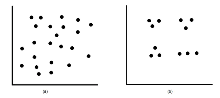
Although for simple scenarios, the process of clustering might appear to be fairly straight-forward, for more general cases, it can be a significantly complex process. Figure 1.1(a) presents an example in which it is difficult to determine appropriate clusters as well as the number of clusters which may suitably reveal the data structure. On the other hand, in figure 1.1(b), it is apparent that four clusters are present. The data-driven nature of various applications increases difficulty in designing a universal algorithm that can accurately and efficiently discover the clusters in the provided data. Also, another factor is the unsupervised nature of the data sets. These kinds of problems encouraged the creation of various types of clustering algorithms such as evolutionary and metaheuristics algorithms. An Evolutionary Algorithm (EA) is a population-based algorithm which is inspired by natural evolution or

(12)

Figure 1.1: Complexity of clustering

the collective behavior of natural self-organizing system (e.g. ant colony, bee colony, bird flocking, fish schooling etc.). Specifically, EAs, when used for clustering, have been shown to provide near-optimal solutions for unsupervised data sets. A large number of algorithms have been created using EAs to solve clustering problems [5–7].

1.4 Clustering Algorithms

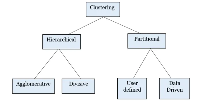
According to [1], there are two main approaches to clustering: partitional clustering and hierarchical clustering. Partitional clustering [8] produces various partitions and keeps eval-uating those partitions using a certain condition (for example, the minimum sum of squares). Hierarchical clustering [9] creates a hierarchy of clusters based on a given dataset using spe-cific criteria. For example, if vehicles represent a class, public transportation vehicles would

(13)

Hierarchical clustering, on the other hand, does not assume the number of clusters before-hand and can be applied to any dataset. However, hierarchical clustering algorithms do not perform well for larger datasets because due to the amount of time and memory complexity requirements. Although various clustering algorithms exist, the selection of an appropriate

Figure 1.2: Taxonomy of clustering methods

algorithm depends on the particular problem.

1.4.1

k

-means

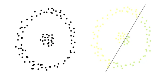
The k-means algorithm is the common choice for clustering large datasets, owing to its low complexity and high execution speed. The main objective of k-means is to associate every data point in the dataset to a prototype point (centroid). Essentially, the prototype point acts as a representative of its cluster. Although, the algorithm is simple and efficient, the drawback of k-means is that it does not work well with non-convex datasets. Furthermore,

(14)

the number of clusters, k, has to be specified before execution of the algorithm. The choice ofk usually has a deep impact on the performance of the algorithm. Thek-means algorithm consists of the following steps:

1. Initialize the number of centroids, k, randomly. In some versions of the algorithm the initial centroids are chosen from the dataset

2. Determine the distance between each data point and each one of the k centroids 3. Assign each point to the cluster whose centroid is the closest one

4. Update the positions of centroids towards the center of gravity of their respective clusters

5. Repeat steps 2, 3 and 4 until the centroid positions change less than a user-defined threshold

The objective function for the k-means algorithm is the following:

J = k ∑ j=1 n ∑ i=1 ��x(_ij)−cj��2 (1.1)

In equation 1.1, k is the number of clusters, n is number of data points, and the term ||x(_ij)−cj||2 represents the distance of the i-th data point, which has been assigned to the

j-th cluster, from the j-th centroid.

(15)

clustering using k-means is shown in figure 1.2.

Figure 1.3: Partitions returned by k-means for non-spherical data

The k-means++ algorithm proposed by Arthur and Vassilvitskii [10] starts by picking the k centers one at a time. After that, choosing each point at random with probability proportional to its squared distance from the already chosen centers.

1.4.3

Swarm Intelligence

The collective behavior of ants, bees, fishes, birds and other species, or what is usually called Swarm Intelligence (SI), has been proven a fascinating topic for researchers for quite some time. Usually, SI shows a structured order which is integrated into the system of species. The way the swarms move also appears to possess some characteristics of a single entity [11]. The swarm’s behavior may consist of the following properties:

(16)

3. Collision Avoidance: Swarm members attempt to avoid collision with other nearby swarm members.

4. Velocity Matching: Swarm members attempt to match the velocity of other nearby members.

Algorithms such as Particle Swarm Optimization (PSO) and Ant Colony Optimization (ACO) have been developed in the literature [12, 13] based on the swarm intelligence of bird flocks and ant colonies.

1.4.3.1 Particle Swarm Optimization

Particle Swarm Optimization (PSO) is an iterative computational method based on SI for optimization of nonlinear functions. The original algorithm was proposed by Kennedy and Eberhart (1995) [12]. PSO mimics the bird flocking behavior to find an optimal solution to a certain optimization problem. The algorithm is initialized with a defined number of particles which represent a set of possible solutions for the problem at hand. Each particle has a random velocity and each moves within the solution space in each iteration. The algorithm considers each particle’s personal best position and global best position after every iteration, in order to determine the particle’s velocity. After the initial proposal of PSO, various types of improved variants emerged, focusing on different applications. PSO has also been modified for the purpose of clustering data, and has showed some promising results compared to other algorithms [14–17]

(17)

1.4.3.2 Ant Colony Optimization

Similarly to PSO, Ant Colony Optimization (ACO) is also an iterative computational method for optimization of nonlinear functions, which was proposed by Marco Dorigo (1992) [13]. It is based upon the behavior of ants for seeking a source of food from their colony. Ants leave a trail of pheromone on their way back to the colony after finding food. The ants get attracted to the pheromone and follow the trail in the hope of finding the food source. However, the pheromone trail evaporates quickly, so that the shortest path to the food source gets the highest utilization. This behavior of ants has been put into use as the ACO algorithm for finding the optimal path in a graph space. The concept of ACO has also been used for generating clustering algorithms, some of which have been proved to be working well with different data sets [18–20]

1.4.4

Evolutionary Algorithms

Taking inspiration from nature, EAs use the following general steps to find out the solution to an optimization problem [21, 22]

1. Generate a random initial population

2. Evaluate all individuals from the population

3. Choose the best individuals from the population to generate the next generation 4. Create the next generation

(18)

The basic idea can be described in short as “survival of the fittest”. The most popular types of EAs are Genetic Algorithm and Differential Evolution.

1.4.4.1 Genetic Algorithm

Genetic Algorithm (GA) is one of the popular EAs which relies upon nature inspired op-erations such as selection, crossover, and mutation [23]. Roulette wheel selection [ref] is the widely used selection method which gives every chromosome a space in an imaginary roulette wheel according to their fitness score. It ensures the chromosomes with higher fitness scores are more likely to be selected. Crossover generates children from parent chromosomes, where each child takes one section of each parent’s chromosome. Finally, after selection and crossover, mutation applies a small random change in the new generation of chromosomes, which effectively creates a diversity among the population. The steps followed to generate solutions to an optimization problem using GA can be summarized as follows:

1. Generate initial population

2. Rank and evaluate individual fitness

3. Apply genetic operators such as crossover, mutation or selection on the chromosomes 4. Create population for next generation

5. Repeat steps 2-4 until the best possible solution or a group of solutions, in the case of multi-objective problems, is chosen

(19)

used for data clustering and have showed promising results [27–30].

1.5 Summary

Clustering is the process of grouping data or observations into a number of meaningful groups subject to further processing. In this chapter, the general concepts of various clustering algorithms and have been discussed, and some of the fundamental issues have been presented. Although the Thesis mainly concentrates on PSO andk-means, some additional algorithms which have been used in data clustering have been presented for information purposes. Each clustering model comes with its own advantages and disadvantages. In particular, the algorithms discussed in this chapter, such as PSO and k-means, fall into the class of partitional clustering algorithms. Partitional algorithms are generally more lightweight which make them easily applicable to larger datasets. Some drawbacks of partitional algorithms are the following:

1. They are limited to forming clusters around prototypes

2. The appropriate number of prototypes is subjective and, for some algorithms, has to be inferred using the appropriate cluster validation index

3. Solutions are subject to sub-optimality as they are dependent on the initial positions of the prototypes

(20)

1.6 Organization of Thesis

This thesis consists of four chapters which are organized as follows:

• Chapter 1 introduces reader to the concepts of data clustering and discusses the various algorithms available to do clustering.

• Chapter 2 introduces PSO and summarizes previous work that used PSO for data clustering.

• Chapter 3 explains the proposed improvements and details the performance compar-ison of the algorithm presented by Van Der Merwe and Engelbrecht [17].

• Chapter 4 summarizes the findings of this thesis, discusses its contributions and limitations. Future work has also been discussed in this chapter.

This thesis also contains following two appendices:

• Appendix A provides the MATLAB codes used to generate the results.

• Appendix B provides the acronyms used throughout the thesis, as well as their defi-nitions.

(21)

Chapter 2

Data Clustering and Particle Swarm

Optimization

2.1 Particle Swarm Optimization

Prior to discussing the details of PSO, a few terms are introduced in order to explain the inner working mechanism of the algorithm.

• Objective function: An function, f(x), that is to be optimized with respect toxwithin certain constraints.

• Search Space: A single or multi-dimensional space in which solutions are found based on the objective function, and the constraints.

• Particle: A member of the swarm, associated with a position vector, a velocity vector and a personal best vector.

• Swarm: A set of particles.

• Position: The location of a particle x within the search space, which represents a possible solution to the problem at hand. The position is updated using the following

(22)

equation,

x(t+ 1) =x(t) +v(t+ 1) (2.1)

where,v is the velocity vector, and t is the iteration number.

• Velocity: The speed with which a particle moves within the search space. The veloc-ity, v, specifies the particle’s course of movement. The velocity is updated using the following equation,

Vi(t+ 1) =ω∗Vi(t) +ϕ1∗(Xpbest(t)−Xi(t)) +ϕ2 ∗(Xgbest(t)−Xi(t)) (2.2)

Where,

ω is the inertia weight

ϕ1 & ϕ2 is the accelerating factor

(Xpbest(t)−Xi(t))is the cognitive term

(Xgbest(t)−Xi(t)) is the social term

• Personal Best: The position, pbest, at which a particle achieved the best (maximum or

minimum) objective function till a particular iteration. Each particle has a memory of its own personal best.

• Global Best: The best position vector,g, out of all personal bests in the whole swarm. The pseudocode of the PSO algorithm is presented next:

(23)

Algorithm 1 Basic PSO 1: for each particle do

Randomly Initialize particle and velocity 2: end for

3: while maximum iterations or minimum error criteria is not attained do

4: for each particle do

5: Find the particle with the best fitness p in the swarm 6: Calculate particle velocity according to the equation 2.2 7: Apply the velocity limit

8: Update particle position according to the equation 2.1 9: Apply the position limit

10: Update velocity and position 11: end for

12: end while

13: return p

The objective of PSO is to improve the position vectors and find a global best g where g =argmin(f(x)).

2.2 PSO and Data Clustering

An early PSO-based clustering algorithm was proposed by Van Der Merwe and Engelbrecht in 2003 [17]. In this algorithm, a data vector,y, is represented as anM-dimensional column vector. Thei-th particle is represented by a group of column vectors,xi ={pi1, pi2, ..., pinc}, where pin, n = 1,2, …, nc, is a potential centroid vector, and nc denotes the number of

centroids. The swarm’s initial position can be either determined by k-means or can be chosen randomly.

In [17], k-means was used to initialize the particles. After initialization, the particles obtained from k-means where added to a population of particles obtained randomly. Then, the algorithm applies generic PSO to find out which particle has the best distances from the

(24)

data points.

They evaluated PSO and the Hybrid clustering algorithm during the experiments. The algorithms were compared against K-means on six classification problems in [17]. Their clustering results were compared using three quality measures namely quantization error, intra-cluster distances and inter-cluster distances. The classification problems were composed by two bi-dimensional artificial and four well-known datasets.

The results of this experiments showed that the algorithms of [17], in general, are better than k-Means. Both proposed algorithms converge to lower quantization error in the first artificial problem. The Hybrid clustering algorithm has the smallest quantization error for all proposed datasets. Also, the Hybrid algorithm presents the smallest Inter-cluster Distances. The pseudocode of the standard PSO data clustering algorithm presented in [17] is pre-sented below:

Algorithm 2 Standard Data Clustering PSO 1: for each particle do

3: while maximum iterations/minimum error is not attaineddo

5: for each data pointdo

6: Calculate distance between all data and centroids 7: Assign each data point to the closest centroid 8: end for

9: Update global and local best positions 10: end for

12: Update velocity and position 13: end for

14: end while 15: return p

(25)

2.3 Particle Swarm Clustering

Cohen and de Castro proposed an improved way of clustering using PSO, and they named it Particle Swarm Clustering (PSC) [16]. The algorithm is evaluated with benchmark datasets and results are compared with that of standard unsupervised clustering algorithms. In PSC, PSO is modified to work with clustering and hence differs from PSO in a sense that unlike PSO, where each particle in the space leads to a potential solution and finally encodes the whole solution, PSC considers each particle as representation of clusters and thus encodes part of the solution. The performance evaluation measure in PSC differs from the fitness quality function used in the general PSO. Rather it initializes particles and then move these particles into such regions which shall represent natural clusters. Equation(2.3) represents a modified form of PSO and is the math equation used in PSC.

Vi(t+ 1) =ω∗Vi(t) +ϕ1∗(Xpbest(t)−Xi(t)) +ϕ2∗(Xgbest(t)−Xi(t)) +ϕ3∗(yj−xi(t)) (2.3)

where,

vi(t)is Particle’s previous position

pi(t) -xi(t)is the cognitive term

gj(t) - xi(t)is the social term

yj(t) - xi(t) is the self-organizing term

The particle swarm clustering algorithm has five main input parameters which are given in the following pseudo code. These are 1) the dataset which is going to be clustered, 2)

(26)

maximum number of iterations, 3) number of particles, 4) maximum velocity, and 5) initial value of the learning parameter.

1: procedure PSC 2: for each particle do

4: while maximum iterations or minimum error criteria is not attained do

6: Find the particle with the best fitness p in the swarm 7: end for

8: end while

9: return p

10: end procedure

Initially, the parameters of velocity and particles (cluster’s centroids) are randomly cho-sen, with maximum bound on the velocity values already defined. Then the distances between nearest data items are calculated and data items with minimum distance are grouped to-gether to form clusters. After each iteration, the velocity, distance and centroids of clusters are updated until convergence.

The authors evaluated the algorithm using the Ruspini dataset which has 75 components in a two-dimensional space. The dataset was first normalized into the range of [0,1]. Then, the parameters were initialized and the PSC algorithm run for the specified number of iterations, which clustered the whole dataset correctly into four groups. It was shown that there were 20, 23, 17 and 15 data items into four clusters, respectively. The number of iterations were 150, and the maximum velocity was set to 0.001. The number of iterations, the maximum velocity, and the number of particles affected the overall performance of the

(27)

29 data items, and the clustering performance is compared with k-means clustering. It was shown that PSC clusters the data more efficiently and addresses the problem of stagnation which other algorithms had.

Another concern that PSC handled is that data is sparse, and we often encounter cases where data items do not belong to any cluster. To handle this problem, PSC moves such data items in the direction of the cluster with the maximum number of data items. Apart from the number of iterations and maximum velocity parameters, the social and cognitive terms also affected clustering. So, instead of randomly initializing these terms, values were changed in a fixed interval as follows:

ϕ1, ϕ2 ∈[0.1 2.05] and ϕ3 ∈ [0.005 1]

To determine the effect of varying the above parameters in their specified range, all the other parameters are kept constant as given below:

• Number of particles were fixed to 8

• Maximum velocity was initialized to 0.01 • Number of iterations were initialized to 200 • Inertia weight ω= 0.95

• social ϕ1 and cognitive ϕ2 terms were fixed to 0

• Self-organizing terms ϕ3 = 0.005

After running PSC, it was observed that many of the particle got stuck to their positions and become stationary, which affected the clustering performance. On the other hand, when

(28)

the social and cognitive terms were also introduced in the PSC algorithm, clustering was improved. Thus, it can be concluded that only introducing the self-organizing term and fixing social and cognitive terms to 0 leads to poor clustering results whereas introducing all of the three terms results in better clustering performance. This indicates that the social and cognitive terms contribute significantly in the clustering process. It was also concluded that the fixed initialization of all terms leads to poor clustering as opposed to random initialization.

2.4 Cooperative-Multipopulation Data Clustering PSO

Population-based data clustering algorithms employed in dynamic environments, lose the diversity of the population and the outdated memory of the individuals. Georgieva and Engelbrecht in [31] proposed a new particle swarm optimization alternative for clustering in dynamic environments, named cooperative-multipopulation data clustering PSO.

Most of the dynamic population-based clustering algorithms are variations or improve-ments of the static population-based algorithm of [17]. The new clustering algorithm of [31], cooperative-multipopulation data clustering PSO, is actually a combination of two algorithm named Multi-swarm Data Clustering PSO [32] and Cooperative Data Clustering PSO [33].

From the Multi-swarm Data Clustering PSO [32], the new algorithm takes the repulsion and anti-convergence methods. The repulsion method is the re-initialization of a swarm

(29)

proposed in [34], where a proportion of the population is placed in new random positions of the search space.

As for the Cooperative Data Clustering PSO [33], this new dynamic population-based algorithm takes each swarm that optimizes only one centroid. The other algorithms [32], [34] and [17] optimizes all centroid in each swarm. In order to be able to optimize all centroids, [33] proposed a context particle. The context particle is based on the best solutions of each swarm. Because of this context particle, the Cooperative Data Clustering PSO [33] is more viable than Multi-swarm Data Clustering PSO [32].

The cooperative-multipopulation data clustering PSO presented by [31] combines Coop-erative Data Clustering PSO [33] (because of it’s quality) and Multi-swarm Data Clustering PSO [33] (because of it’s robustness). Furthermore, in order to avoid inaccurate representa-tions of the solution, in [31] added an additional swarm, named the “explorer swarm”. The additional swarm substitutes a swarm that will be reinitialized. During this re-initialization, the re-initialized swarm becomes “explorer swarm” and the previous “explorer swarm” takes the place of the re-initialized swarm in the clustering solution. This additional swarm guar-antee that the solution is given by algorithm’s exploration and is not random (given by re-initialization).

The algorithm of the cooperative-multipopulation data clustering PSO is performed using the following steps:

1. Initialize the particles of the k+ 1 swarms (one additional as ”explorer swarm”). 2. Initialize the context particle.

(30)

fitness value is calculated putting the new particle in the context particle. Also, update the swarm best particle if some of the updated particles are better.

4. Update the context particle.

5. Update the position of all particles with the new context particle using standard PSO’s update equations.

6. Verify if two swarms are too close with a minimal inter-cluster distance. Re-initialize one of them in this case and change it by the “explorer swarm”.

7. Verify if a swarm converges too much with a minimal intra-cluster distance. Re-initialize this swarm in this case and change it by the “explorer swarm”.

8. Go to the step 3 until the stopping condition is not reached (max iteration steps). At the end, the resulting context particle is the output of this algorithm.

Then, in [31] an elitist version of their cooperative-multipopulation data clustering PSO algorithm was also proposed. The elitist version only changes the context particle to include new best solutions (not downgrade with re-initialization).

The dataset used for the experimental setup were auto-generated temporal clustering datasets with 8 clusters. Each cluster was changed in a dynamic way, moving patterns from one cluster to another at each interval of change. The algorithms were evaluated on a combination of change frequency between 1 and 5, severities in the same range and dimensions with 3, 8 and 15.

(31)

algorithm ran for 1000 iterations with 50 particles of swarm size. During the re-initialization, only 10% of the swarm was re-initialized.

The authors compared six data clustering PSO algorithms, the standard [17], the stan-dard with re-initialization, Multi-swarm Data Clustering PSO [32], Cooperative Data Clus-tering PSO [33], cooperative-multipopulation data clusClus-tering PSO and it’s elitist version.

Between six population-based clustering algorithms evaluated on pattern migration datasets, according to the Ray-Turi measure, the elitist cooperative-multipopulation data clustering PSO gave the most optimal solution. However, this algorithm didn’t perform well with the increase of dimension. The cooperative-multipopulation algorithm didn’t present good re-sults considering Ray-Turi and intra-cluster distance measures. But, the elitist version gave better results because it controls the effects of re-initialization on the context particle in a better way.

(32)

Chapter 3

Associative Data Clustering PSO

3.1 Improving Swarm Association

An issue with the basic data clustering PSO-based algorithm presented in [17] is the associ-ation problem that arises when calculating the square of the Euclidean distance,Ji, between

the centroid vectors within theith _particle,_x

i, and those within the global best particle,gbest.

More specifically, each particle should be represented as a set of centroids, in the sense that the order of centroid vectors within the particle should be of no importance. However, for the purpose of implementingJi, centroid vectors may be ordered. In [17], there is no indication

that a solution to the association problem has been considered. The square distance, Ji, is

calculated using the following equation:

Ji = nc

∑

j=1

||xj_i−g_bestj ||2 (3.1)

where nc is the number of centroids, and xji and g j

best represent the jth centroid within the

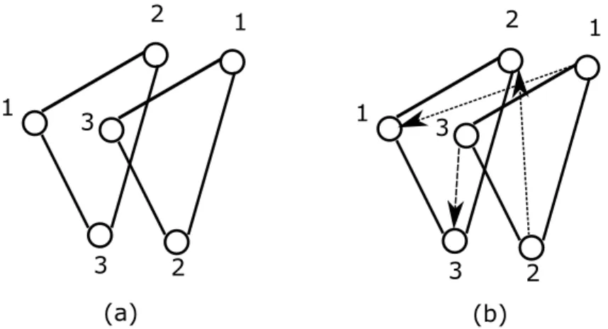
particle and the global best particle, respectively. An example illustrating the aforementioned association problem is shown in Figure 3.1.

(33)

1 2 ₁ 2 3 3 1 2 ₁ 2 3 3 (a) (b)

Figure 3.1: (a) Sample positions of global best and particle, (b) Particle movement towards global best

centroids are associated with the same particle. The numbers indicate the order of the centroid vector within the particle. In the case that a proper centroid association is not used, it is apparent that the particle will have to undergo a relatively large change in order to match the global best particle. This motion is indicated by the arrows in Figure 3.1(b). Nevertheless, the positions of the centroids within the two particles are in fact close to each other if an appropriate centroid associate association technique is implemented.

3.1.1

Data Clustering PSO with Association

In order to mitigate the association issue, a modification to [17] has been proposed. The overall modified algorithm is presented in Algorithm 3. In particular, the modified step is also described in more detail in Algorithm 4. Based on this modification, the global best solution corresponding to theith _{particle is represented as}_g_ˆj

best,i. Therefore, the equation for

calculating the square Euclidean distance becomes as follows:

ˆ Ji =

nc

∑

(34)

The algorithm for ADCPSO is shown in Algorithm 3 and the inner algorithm of the modified portion of DCPSO has been shown in Algorithm 4.

Algorithm 3 Associative Data Clustering PSO 1: for each particle do

3: while maximum iterations/minimum error is not attaineddo 4: for each particle do

5: for each data pointdo

6: Calculate distance between all data and centroids 7: Assign each data point to the closest centroid 8: end for

9: Update global and local best positions 10: end for

12: Determine distances between global best centroids 13: and specific particle’s centroids

14: Rearrange global best, gbest, centroids

15: according to the distances between centroids 16: Update velocity and position

17: end for

18: end while 19: return p

Algorithm 4 Association Fix for Data Clustering PSO 1: nc centroids

3: Initialize allnc labels to 0

4: foreach centroid in the particle do

5: if label is 0 then

6: foreach centroid in global best do

7: measure distance between particle centroid and global best centroid

8: end for

9: end if

10: append global best centroid with smallest distance to new global best 11: Set label to 1 for the chosen global best centroid

12: end for

(35)

3.1.2

Experimental Setup

A computer with Intel© Core i5-3230M with MATLAB R2016b has been used to simulate all experiments presented in the next section. Several standard datasets have been used in the experiments to evaluate the performance clustering algorithms. The details for the datasets used are mentioned in table 3.1. All of the datasets, except for the artificial dataset, are publicly available at UCI Machine Learning Repository [35].

Table 3.1: Datasets used for evaluation

Dataset Objects Attributes

Ruspini 75 2

Artificial 200 2

Iris 150 4

Automotive 240 8

Sonar 208 60

The following were the parameters for the programs in MATLAB:

• Maximum Clusters: 3 • Particles: 20, 40, 60 • Inertia: 0.99 • Maximum Iterations: 500 • Program Evaluation: 500 • Accelerating factors: 0.5 • Dimensions: 2, 4, 8, 60

(36)

3.1.3

Results and Comparison

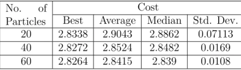
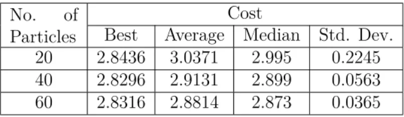
Tables 3.2-11 report the values of the best, average, median, and standard deviation of the global best cost found using 20, 40, and 60 particles, considering 500 runs of the algorithms. A total of five different datasets were used. In general, it can be observed that ADCPSO has achieved a lower cost against the DCPSO. Also, the standard deviation of the ADCPSO was lower than that of DCPSO, which indicates that the performance of DCPSO was more sensitive to particle initialization. Another important point is that the improvement of ADCPSO with respect to DCPSO increases as the dataset dimension increases. Table 3.16 reports the overall percentage improvement of ADCPSO against the DCPSO.

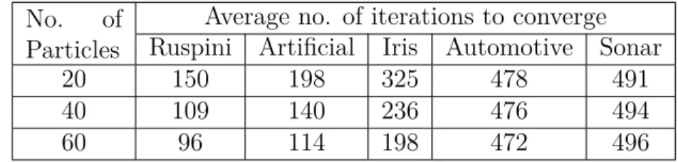
Table 3.12-15 presents the average execution time and number of iteration to converge required per run. It is apparent that ADCPSO has a disadvantage compared to DCPSO. Although the number of iterations required by ADCPSO in order to converge is in general smaller compared to DCPSO, its overall execution time is higher. The reason is that indi-vidual iterations of ASCPSO are more expensive computationally compared to DCPSO. For this reason, we have proposed another improved version of ADCPSO, namely IADCPSO. In particular, IADCPSO exhibits improved execution times, which comes at the expense of additional memory storage requirements. The extra memory storage is simply equal to the one required for storing the personal bests. The IADCPSO algorithm is described in section 3.2.

(37)

Table 3.2: Results for Ruspini dataset for the ADPSO algorithm No. of

Particles

Cost

Best Average Median Std. Dev. 20 2.9782 3.0978 2.9843 0.1691 40 2.9781 3.0811 2.9806 0.1315 60 2.9781 3.084 2.9804 0.1323

Table 3.3: Results for Ruspini dataset for the DCPSO algorithm No. of

Particles

Cost

Table 3.4: Results for Artificial dataset for the ADCPSO algorithm No. of

Particles

Cost

Table 3.5: Results for Artificial dataset for the DCPSO algorithm No. of

Particles

Cost

Table 3.6: Results for Iris dataset for the ADCPSO algorithm No. of

Particles

Cost

(38)

Table 3.7: Results for Iris dataset for the DCPSO algorithm No. of

Particles

Cost

Table 3.8: Results for Automotive dataset for the ADCPSO algorithm No. of

Particles

Cost

Table 3.9: Results for Automotive dataset for the DCPSO algorithm No. of

Particles

Cost

Table 3.10: Results for Sonar dataset for the ADCPSO algorithm No. of

Particles

Cost

Table 3.11: Results for Sonar dataset for the DCPSO algorithm No. of

Particles

Cost

Best Average Median Std. Dev. 20 383.6466 404.0151 403.3845 9.5313 40 373.7812 386.0607 385.2033 6.0774

(39)

Table 3.12: ADCPSO run time No. of

Particles

Average time of each iteration (seconds) Ruspini Artificial Iris Automotive Sonar

20 0.266 0.304 0.495 0.696 1.525

40 0.448 0.484 0.781 0.448 3.109

60 0.586 0.643 1.015 1.999 4.685

Table 3.13: DCPSO run time No. of

Particles

20 0.194 0.227 0.335 0.462 1.317

40 0.301 0.360 0.630 0.255 2.570

60 0.406 0.492 0.864 1.348 3.848

Table 3.14: ADCPSO average number of iterations for convergence No. of

Particles

Average no. of iterations to converge Ruspini Artificial Iris Automotive Sonar

20 150 198 325 478 491

40 109 140 236 476 494

60 96 114 198 472 496

Table 3.15: ADCPSO average number of iterations for convergence No. of

Particles

20 193 269 392 481 490

40 131 193 360 485 495

60 112 168 321 485 497

Table 3.16: Improvement achieved by ADCPSO against DCPSO (%) No. of

Particles

Best Cost Improvement (%)

Ruspini Artificial Iris Automotive Sonar

20 0 0 0.34 1.1 1.95

40 0 0 0.08 0.45 1.61

(40)

3.2 Improved ADCPSO (IADCPSO)

3.2.1

Reducing Execution Time

The drawback of ADCPSO is that the program runs take longer than DCPSO due to its higher computational complexity. To remedy this issue, an additional modification to the algorithm has been proposed, so that the association part of the algorithm runs only when there is a change in the global best solution. In order to achieve this objective, all of the updated global best vectors, gˆj_best,i are stored as separate variables. Therefore, there will be one global vector stored per particle. The additional memory requirements equal the memory needed to store the personal best vectors for all particles. Essentially, there is a trade off between memory and execution time.

3.2.2

Results and Comparison

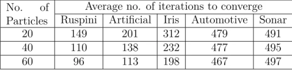
Tables 3.17-19 represent the best cost achieved by IADCPSO, the average time for each iter-ation, and the average number of iterations needed for convergence. The results demonstrate that IADCPSO exhibits almost the same cost as ADCPSO, while reducing the execution time close to that of the DCPSO algorithm.

Table 3.17: Best cost achieved by Improved ADCPSO No. of

Particles

Best Cost Improvement

Ruspini Artificial Iris Automotive Sonar 20 2.978 7.7115 2.832 15.683 373.925 40 2.978 7.7114 2.828 15.592 370.53

(41)

Table 3.18: Execution time for IADCPSO No. of

Particles

20 0.161 0.207 0.304 0.497 1.38

40 0.265 0.324 0.506 0.99 2.73

60 0.364 0.427 0.682 1.455 4.25

Table 3.19: IADCPSO average number of iterations needed for convergence No. of

Particles

20 149 201 312 479 491

40 110 138 232 477 495

(42)

Chapter 4

Conclusions and Future Work

4.1 Primary Findings

This research aimed to improve a PSO based data clustering algorithm. One major issue with several existing PSO-based clustering algorithms was identified. The issue was the association of particle centroids with the centroids of the global best particle when computing the cognitive term. We have proposed a modification to the PSO clustering algorithm in [17]. We performed comparisons between the proposed ADCPSO and the existing DCPSO. In summary, ADCPSO showed slight to moderate improvement, in terms of the cost, for datasets with dimensions higher than 3. Also, the proposed algorithm converged faster than the original DCPSO, in terms of the number of iterations. The only drawback was that the execution time per iteration was higher for ACPSO. This was due to the fact that individual iterations required additional computations for performing centroid associations between particles and the global best vector. This concern was also mitigated in this thesis in an second modified algorithm, namely IADCPSO.

(43)

4.2 Recommendations for Future Work

As this thesis focused on the use of PSO to cluster datasets, various future work can be done based on this research:

• Applying the association operation between the particles and their personal best, in addition to the association operation between the particles and the global best, • Studying the scalability of the algorithms,

• Comparing the performance of IADCPSO with additional existing PSO-based cluster-ing algorithms,

• Implementing advanced PSO-based dimensional clustering algorithms, similar to the one proposed in [36]

(44)

Bibliography

[1] A. K. Jain, M. N. Murty, and P. J. Flynn, “Data clustering: a review,”ACM computing surveys (CSUR), vol. 31, no. 3, pp. 264–323, 1999.

[2] P. Dayan, M. Sahani, and G. Deback, “Unsupervised learning,” The MIT encyclopedia of the cognitive sciences, 1999.

[3] A. K. Jain, “Data clustering: 50 years beyond k-means,” Pattern recognition letters, vol. 31, no. 8, pp. 651–666, 2010.

[4] A. K. Jain and R. C. Dubes, Algorithms for clustering data. Prentice-Hall, Inc., 1988.

[5] M. J. Abul Hasan and S. Ramakrishnan, “A survey: hybrid evolutionary algorithms for cluster analysis,” Artificial Intelligence Review, vol. 36, no. 3, pp. 179–204, 2011. [6] A. A. Freitas, “A survey of evolutionary algorithms for data mining and knowledge

discovery,” inAdvances in evolutionary computing, pp. 819–845, Springer, 2003.

[7] E. R. Hruschka, R. J. Campello, A. A. Freitas, et al., “A survey of evolutionary algo-rithms for clustering,” IEEE Transactions on Systems, Man, and Cybernetics, Part C (Applications and Reviews), vol. 39, no. 2, pp. 133–155, 2009.

(45)

[9] A. D. Gordon, “Hierarchical classification,” inClustering and classification, pp. 65–121, World Scientific, 1996.

[10] D. Arthur and S. Vassilvitskii, “k-means++: The advantages of careful seeding,” in Proceedings of the eighteenth annual ACM-SIAM symposium on Discrete algorithms, pp. 1027–1035, Society for Industrial and Applied Mathematics, 2007.

[11] I. D. Couzin, J. Krause, R. James, G. D. Ruxton, and N. R. Franks, “Collective memory and spatial sorting in animal groups,” Journal of theoretical biology, vol. 218, no. 1, pp. 1–11, 2002.

[12] J. Kennedy and R. Eberhart, “Particle swarm optimization,” in Proc. Conf. IEEE Int Neural Networks, vol. 4, pp. 1942–1948 vol.4, 1995.

[13] M. Dorigo, “Optimization, learning and natural algorithms,”Ph. D. Thesis, Politecnico di Milano, Italy, 1992.

[14] A. Szabo, L. N. de Castro, and M. R. Delgado, “The proposal of a fuzzy clustering algorithm based on particle swarm,” in Nature and Biologically Inspired Computing (NaBIC), 2011 Third World Congress on, pp. 459–465, IEEE, 2011.

[15] A. Szabo, A. K. F. Prior, and L. N. de Castro, “The proposal of a velocity memoryless clustering swarm,” inEvolutionary Computation (CEC), 2010 IEEE Congress on, pp. 1– 5, IEEE, 2010.

[16] S. C. Cohen and L. N. de Castro, “Data clustering with particle swarms,” inEvolutionary Computation, 2006. CEC 2006. IEEE Congress on, pp. 1792–1798, IEEE, 2006.

(46)

[17] D. Van der Merwe and A. P. Engelbrecht, “Data clustering using particle swarm opti-mization,” inEvolutionary Computation, 2003. CEC’03. The 2003 Congress on, vol. 1, pp. 215–220, IEEE, 2003.

[18] R. S. Parpinelli, H. S. Lopes, and A. A. Freitas, “Data mining with an ant colony optimization algorithm,”IEEE Transactions on evolutionary computation, vol. 6, no. 4, pp. 321–332, 2002.

[19] P. Shelokar, V. K. Jayaraman, and B. D. Kulkarni, “An ant colony approach for clus-tering,” Analytica Chimica Acta, vol. 509, no. 2, pp. 187–195, 2004.

[20] P. Rocca, L. Manica, and A. Massa, “An improved excitation matching method based on an ant colony optimization for suboptimal-free clustering in sum-difference compromise synthesis,” IEEE Transactions on Antennas and Propagation, vol. 57, no. 8, pp. 2297– 2306, 2009.

[21] K.-C. Wong, “Evolutionary algorithms: Concepts, designs, and applications in bioinfor-matics: Evolutionary algorithms for bioinformatics,” arXiv preprint arXiv:1508.00468, 2015.

[22] F. Streichert, “Introduction to evolutionary algorithms,” paper to be presented Apr, vol. 4, 2002.

(47)

[25] S. Iqbal and M. T. Hoque, “A homologous gene replacement based genetic algorithm,” inProceedings of the 2016 on Genetic and Evolutionary Computation Conference Com-panion, pp. 91–92, ACM, 2016.

[26] S. Iqbal and M. T. Hoque, “An adaptive and memory-assisted local crossover in genetic algorithm,” tech. rep., University of New Orleans, 2017.

[27] L. A. N. Lorena and J. C. Furtado, “Constructive genetic algorithm for clustering prob-lems,” Evolutionary Computation, vol. 9, no. 3, pp. 309–327, 2001.

[28] C. Ding, Y. Cheng, and M. He, “Two-level genetic algorithm for clustered traveling salesman problem with application in large-scale tsps,” Tsinghua Science & Technology, vol. 12, no. 4, pp. 459–465, 2007.

[29] A. Mukhopadhyay, U. Maulik, and S. Bandyopadhyay, “Multiobjective genetic algorithm-based fuzzy clustering of categorical attributes,”IEEE Transactions on Evo-lutionary Computation, vol. 13, no. 5, pp. 991–1005, 2009.

[30] C.-H. Cheng, W.-K. Lee, and K.-F. Wong, “A genetic algorithm-based clustering ap-proach for database partitioning,” IEEE Transactions on Systems, Man, and Cybernet-ics, Part C (Applications and Reviews), vol. 32, no. 3, pp. 215–230, 2002.

[31] K. Georgieva and A. P. Engelbrecht, “A cooperative multi-population approach to clus-tering temporal data,” in Evolutionary Computation (CEC), 2013 IEEE Congress on, pp. 1983–1991, IEEE, 2013.

(48)

[33] F. Van den Bergh and A. P. Engelbrecht, “A cooperative approach to particle swarm optimization,” IEEE transactions on evolutionary computation, vol. 8, no. 3, pp. 225– 239, 2004.

[34] R. C. Eberhart and Y. Shi, “Tracking and optimizing dynamic systems with particle swarms,” in Evolutionary Computation, 2001. Proceedings of the 2001 Congress on, vol. 1, pp. 94–100, IEEE, 2001.

[35] M. Lichman, “UCI machine learning repository,” 2013.

[36] S. Kiranyaz, T. Ince, A. Yildirim, and M. Gabbouj, “Fractional particle swarm opti-mization in multidimensional search space,”IEEE Transactions on Systems, Man, and Cybernetics, Part B (Cybernetics), vol. 40, no. 2, pp. 298–319, 2010.

(49)

Appendix A

MATLAB Codes

A.1 Data Clustering PSO

1 % %%%%%%%%%%%%%%%%%%%%%%%%%%%%%%%%%%%%%%%%%%%%%%%%%%%%%%%%%%%%%%%%%%%%%%%%% 2 % %%%%%%%% Van Der Merwe & Engelbrecht 's PSO clustering %%%%%%%%%%%%%%%%%%% 3 % %%%%%%%%%%%%%%%%%%%%%%%%%%%%%%%%%%%%%%%%%%%%%%%%%%%%%%%%%%%%%%%%%%%%%%%%% 4

5 for p =1:500 6

7 data_set = textread ('data_set_sonar.txt '); % Import Dataset 8 dataset_subset =0; 9 n_dimensions =60; 10 max_iter =500; 11 vmax =0 .01; 12 w=0 .99; 13 global Y 14 15 phi1 =0 .5; % 1.1; 16 phi2 =0 .5; % 0.8; 17 phi3 =0 .005; % 0.3;

(50)

18 phi4 =0 .06;

19 %Y=rand( length (Y) ,2); 20 N=max(size( data_set )); 21 Y= zeros (N, n_dimensions ); 22 for i=1: n_dimensions

23 Y(:,i)= data_set (:,i)/max( data_set (:,i));

24 end 25 n_centroids =3; 26 n_particles =60; 27 28 tic 29 v=cell( n_particles ,1); 30

31 for i=1: n_particles

32 v{i}= vmax *(2* rand( n_centroids , n_dimensions ) -1);

33 end

34

35 x=cell( n_particles ,1); 36 for i=1: n_particles 37 for j=1: n_centroids

38 r=ceil(rand (1 ,1) *( length (Y) -1) +1); 39 x{i}(j ,:)=Y(r ,:);

40 end

(51)

45 personal_bests = x; 46 global_best_cost =1 e99;

47 global_best = inf( n_centroids , n_dimensions ); 48

49 prev_global_best_cost =inf; 50 iter =0;

51 run_flag =1;

52 while (iter < max_iter && run_flag ==1) 53 run_flag =0;

54 for iter_inner =1:50 55 iter=iter +1;

56 % Particle loop

58 % Centroid loop

59 for j=1: n_centroids

60 Distance {i}(j ,:) =( sum (( repmat (x{i}(j ,:) ,[N ... 1]) -Y).^2 ,2)). ';

61 end

62 end

64 [ minimum_dist_temp , closest_centroid_temp ]= ... min( Distance {i} ,[] ,1);

65 minimum_dist (i ,:)= minimum_dist_temp ;

66 closest_centroid (i ,:)= closest_centroid_temp ;

67 end

(52)

70 prev_global_best_cost = global_best_cost ; 71 for i=1: n_particles

72 if total_minimum (i) < personal_best_cost (i) 73 personal_best_cost (i)= total_minimum (i); 74 personal_bests {i} = x{i};

75 end

76 if total_minimum (i) < global_best_cost 77 global_best_cost = total_minimum (i); 78 global_best = x{i}; 79 end 80 81 end 82 83

84 for i=1: n_particles 85

86 v{i} = v{i} ...

87 + phi1 *( personal_bests {i} - x{i}) + ... phi2 *( global_best - x{i});

88 x{i} = x{i}+w*v{i}; 89

90

91 end

(53)

96 c_iter =iter; 97 run_flag =1; 98 end 99 end 100 end 101 end

A.2 Data Clustering PSO with

k

-means

1 % %%%%%%%%%%%%%%%%%%%%%%%%%%%%%%%%%%%%%%%%%%%%%%%%%%%%%%%%%%%%%%%%%%%%%%%%% 2 % %%%%% Van Der Merwe & ’Engelbrechts PSO clustering with k- means %%%%%%%% 3 % %%%%%%%%%%%%%%%%%%%%%%%%%%%%%%%%%%%%%%%%%%%%%%%%%%%%%%%%%%%%%%%%%%%%%%%%% 4

5 for p =1:500 6

7 data_set = textread ('data_set_sonar.txt '); % Ruspini Dataset 8 dataset_subset =0; 9 n_dimensions =60; 10 max_iter =500; 11 vmax =0 .01; 12 w=0 .99; 13 global Y 14 15 phi1 =0 .5; % 1.1;

(54)

17 phi3 =0 .005; % 0.3; 18 phi4 =0 .06;

19 N=max(size( data_set )); 20 Y= zeros (N, n_dimensions ); 21 for i=1: n_dimensions

23 end 24 n_centroids =3; 25 n_particles =60; 26 27 tic 28 v=cell( n_particles ,1); 29

32 end

33

39 end

(55)

44 personal_bests = x; 45 global_best_cost =1 e99;

50 run_flag =1;

55 % Particle loop

57 % Centroid loop

60 end

61 end

66 end

(56)

74 end

75 if total_minimum (i) < global_best_cost 76 global_best_cost = total_minimum (i); 77 global_best = x{i};

78 end

79

80 end

81

84 v{i} = v{i} ...

85 + phi1 *( personal_bests {i} - x{i}) + ... phi2 *( global_best - x{i});

86 x{i} = x{i}+w*v{i};

87 end

88 w=w*0 .99; 89

90 if (abs( global_best_cost - prev_global_best_cost ) >0.001) 91

(57)

95 end

96 end

97 time=toc; 98 for i=1:3

99 [indices , global_best , SumD] = kmeans (Y,3,'start ',global_best ); 100 global_best_cost_kmeans =sum(SumD);

101 end

102 end

A.3 Associative DCPSO

1 % %%%%%%%%%%%%%%%%%%%%%%%%%%%%%%%%%%%%%%%%%%%%%%%%%%%%%%%%%%%%%%%%%%%%%%%%% 2 % %%%%%%%%%%%%%%%%%%%%%%%%%%%%% ADCPSO %%%%%%%%%%%%%%%%%%%%%%%%%%%%%%%% 3 % %%%%%%%%%%%%%%%%%%%%%%%%%%%%%%%%%%%%%%%%%%%%%%%%%%%%%%%%%%%%%%%%%%%%%%%%% 4 for p =1:500

5

6 data_set = textread ('data_set_sonar.txt '); 7 dataset_subset =0; 8 n_dimensions =60; 9 max_iter =500; 10 vmax =0 .01; 11 w=0 .99; 12 global Y 13

(58)

15 phi2 =0 .5; % 0.8; 16 phi3 =0 .005; % 0.3; 17 phi4 =0 .06;

18 N=max(size( data_set )); 19 Y= zeros (N, n_dimensions ); 20 for i=1: n_dimensions

22 end 23 24 n_centroids =3; 25 n_particles =60; 26 27 tic 28 v=cell( n_particles ,1); 29

32 end

33

(59)

42 motion_iter =[];

43 personal_best_cost = linspace (1e99 ,1e99 , n_particles ); 44 personal_bests = x;

45 global_best_cost =1 e99;

50 run_flag =1;

55 % Particle loop

57 % Centroid loop

60 end

61 end

(60)

67 total_minimum =sum( minimum_dist ,2); 68

74 end

75 if total_minimum (i) < global_best_cost 76 global_best_cost = total_minimum (i); 77 global_best = x{i}; 78 end 79 80 end 81 gtemp = global_best *0; 82

85 label = zeros (1, n_centroids ); 86 for j=1: n_centroids

87 d1=inf;

88 for c=1: n_centroids 89 if (label (c)==0)

90 d=sum ((x{i}(j ,:) -global_best (c ,:)).^2);

(61)

94 end

95 end

96 end

97 gtemp (j ,:)= global_best (ctemp ,:); 98 label (:, ctemp )=1;

99 end

100

101

102 v{i} = v{i} ...

103 + phi1 *( personal_bests {i} - x{i}) + phi2 *( gtemp - ... x{i});

104 x{i} = x{i}+w*v{i};

105 end

106 w=w*0 .99; 107

108 if (abs( global_best_cost - prev_global_best_cost ) >0.001) 109 110 c_iter =iter; 111 run_flag =1; 112 end 113 end 114 end 115 time=toc; 116 end

(62)

A.4 ADCPSO with

k

-means

1 % %%%%%%%%%%%%%%%%%%%%%%%%%%%%%%%%%%%%%%%%%%%%%%%%%%%%%%%%%%%%%%%%%%%%%%%%% 2 % %%%%%%%%%%%%%%%%%%%%%%% ADCPSO with k-means %%%%%%%%%%%%%%%%%%%%%%%%%% 3 % %%%%%%%%%%%%%%%%%%%%%%%%%%%%%%%%%%%%%%%%%%%%%%%%%%%%%%%%%%%%%%%%%%%%%%%%% 4 for p =1:500

5

6 data_set = textread ('data_set_sonar.txt '); 7 dataset_subset =0; 8 n_dimensions =60; 9 max_iter =500; 10 vmax =0 .01; 11 w=0 .99; 12 global Y 13 14 phi1 =0 .5; % 1.1; 15 phi2 =0 .5; % 0.8; 16 phi3 =0 .005; % 0.3; 17 phi4 =0 .06; 18 N=max(size( data_set )); 19 Y= zeros (N, n_dimensions ); 20 for i=1: n_dimensions

(63)

24 n_particles =60; 25

26 tic

27 v=cell( n_particles ,1); 28

31 end

32

38 end

39 end

40

41 motion_iter =[];

49 run_flag =1;

(64)

51 run_flag =0;

54 % Particle loop

56 % Centroid loop

59 end

60 end

65 end

(65)

76 global_best = x{i}; 77 end 78 79 end 80 gtemp = global_best *0; 81

86 d1=inf;

87 for c=1: n_centroids 88 if (label (c)==0)

90 if (d<d1) 91 ctemp =c; 92 d1=d; 93 end 94 end 95 end

96 gtemp (j ,:)= global_best (ctemp ,:); 97 98 label (:, ctemp )=1; 99 end 100 101 v{i} = v{i} ...

(66)

103 + phi1 *( personal_bests {i} - x{i}) + phi2 *( gtemp - ... x{i}); 104 x{i} = x{i}+w*v{i}; 105 106 107 end 108 w=w*0 .99; 109

110 if (abs( global_best_cost - prev_global_best_cost ) >0.001) 111 112 c_iter =iter; 113 run_flag =1; 114 end 115 end 116 end 117 time=toc; 118 for i=1:3

119 [¬, global_best , SumD] = kmeans (Y,3,'start ',global_best ); 120 global_best_cost_kmeans =sum(SumD);

121 end

122 end

(67)

2 % %%%%%%%%%%%%%%%%%%%%%% Improved ADCPSO %%%%%%%%%%%%%%%%%%%%%%%%%%%%%% 3 % %%%%%%%%%%%%%%%%%%%%%%%%%%%%%%%%%%%%%%%%%%%%%%%%%%%%%%%%%%%%%%%%%%%%%%%%% 4

5 for p =1:500 6

7 data_set = textread ('data_set_sonar.txt '); 8 dataset_subset =0; 9 n_dimensions =60; 10 max_iter =500; 11 vmax =0 .01; 12 w=0 .99; 13 global Y 14 15 phi1 =0 .5; % 1.1; 16 phi2 =0 .5; % 0.8; 17 phi3 =0 .005; % 0.3; 18 phi4 =0 .06; 19 N=max(size( data_set )); 20 Y= zeros (N, n_dimensions ); 21 for i=1: n_dimensions

23 end 24 25 n_centroids =3; 26 n_particles =60; 27 tic

(68)

29 v=cell( n_particles ,1); 30

33 end

34

40 end

41 end

42

43 motion_iter =[];

47 global_best = inf( n_centroids , n_dimensions ); 48 global_bests = x;

49

52 run_flag =1;

(69)

56 iter=iter +1;

57 % Particle loop

59 % Centroid loop

62 end

63 end

68 end

71 best_updated =0;

77 end

78 if total_minimum (i) < global_best_cost 79 global_best_cost = total_minimum (i);

(70)

81 best_updated =1; 82 end 83 84 end 85 gtemp = global_best *0; 86

87 for i=1: n_particles 88 if best_updated ==1

91 d1=inf;

92 for c=1: n_centroids 93 if ( label (c)==0)

95 if (d<d1) 96 ctemp =c; 97 d1=d; 98 end 99 end 100 end

101 gtemp (j ,:)= global_best (ctemp ,:); 102 label (:, ctemp )=1;

103 end

104 global_bests {i}= gtemp ;

(71)

108 + phi1 *( personal_bests {i} - x{i}) + ... phi2 *( global_bests {i} - x{i});

109 x{i} = x{i}+w*v{i};

110 end

111 w=w*0 .99; 112

113 if (abs( global_best_cost - prev_global_best_cost ) >0.001) 114 115 c_iter =iter; 116 run_flag =1; 117 end 118 end 119 end 120 time=toc; 121 end

A.6 Particle Swarm Clustering

1 %% Initialization

2 data_set = textread ('data_set_sonar.txt '); 3 max_it =150;

4 vmax =0 .01; 5 n_part =3; 6 w=0 .95;

(72)

8 global Y 9 10 phi1 =0; % 1.1; 11 phi2 =0; % 0.8; 12 phi3 =0 .005; % 0.3; 13 phi4 =0 .06; 14

15 Y = [ data_set (: ,1)/max( data_set (: ,1)) ... data_set (: ,2)/max( data_set (: ,2))];

16 N=max(size( data_set ));

17 x=rand( n_cluster_per_particle *n_part ,2); % usually every particle ...

xi initialized at random

18 c = reshape (x,1, []); 19

20 v=vmax *(2* rand( n_part * n_cluster_per_particle ,2) -1); % at random , vi ...

in [-vmax ,vmax]

21 distYX = linspace (1e99 ,1e99 , n_part ); 22 pI =[0 0];

23 pG =[0 0];

24 win_counter = zeros (max(size(x)) ,1);

25 t=1;

26

27 while t < max_it

28 win_counter = zeros ( n_part * n_cluster_per_particle ,1);

(73)

32 end

33 distMatrix (:,i)= distYX ;

34 for k=1: n_cluster_per_particle

35 particle = mat2cel

Improving a Particle Swarm Optimization-based Clustering Method

ScholarWorks@UNO

Dedication

Contents

List of Tables vi

3 Associative Data Clustering PSO 23

List of Tables

List of Figures

Introduction

1.3 Complexity of Clustering Problem

-means

Swarm Intelligence

1.4.3.1 Particle Swarm Optimization

Evolutionary Algorithms

1.4.4.1 Genetic Algorithm

1.5 Summary

1.6 Organization of Thesis

Chapter 2

2.2 PSO and Data Clustering

2.3 Particle Swarm Clustering

2.4 Cooperative-Multipopulation Data Clustering PSO

Chapter 3

Data Clustering PSO with Association

Experimental Setup

Dataset Objects Attributes

Results and Comparison

3.2 Improved ADCPSO (IADCPSO)

Results and Comparison

Chapter 4

Bibliography

Appendix A

A.2 Data Clustering PSO with

A.3 Associative DCPSO

A.4 ADCPSO with

A.6 Particle Swarm Clustering