Training Algorithms for Multilingual Latent Dirichlet Allocation

(1)

Instructor

Training Algorithms for Multilingual Latent Dirichlet

Alloca-tion

Haibo Jin

Helsinki May 12, 2016

UNIVERSITY OF HELSINKI Department of Computer Science

(2)

Faculty of Science Department of Computer Science Haibo Jin

Training Algorithms for Multilingual Latent Dirichlet Allocation Computer Science

May 12, 2016 50 pages + 0 appendices

Multilingual Latent Dirichlet Allocation, Training, Gibbs Sampling, Variational Inference

Multilingual Latent Dirichlet Allocation (MLDA) is an extension of Latent Dirichlet Allocation (LDA) in a multilingual setting, which aims to discover aligned latent topic structures of a par-allel corpus. Although the two popular training algorithms of LDA, collapsed Gibbs sampling and variational inference, can be naturally adopted to MLDA, the two algorithms both become time-inecient with MLDA due to its special structure. To address this problem, we propose an approximate training framework of MLDA, which works with both collapsed Gibbs sampling and variational inference. Through the experiments, we show that the proposed training framework is able to reduce the training time of MLDA considerably, especially when there are many languages. We also summarize the scenarios where the approximate framework gives comparable model accu-racy to that of the standard framework. Finally, we discuss several possible explorations as a future plan.

ACM Computing Classication System (CCS):

Computing methodologies - Machine learning - Machine learning approaches - Learning in proba-bilistic graphical models - Bayesian network models

Applied computing - Document management and text processing - Document capture - Document analysis

Tekijä Författare Author Työn nimi Arbetets titel Title

Oppiaine Läroämne Subject

Työn laji Arbetets art Level Aika Datum Month and year Sivumäärä Sidoantal Number of pages Tiivistelmä Referat Abstract

Avainsanat Nyckelord Keywords

Säilytyspaikka Förvaringsställe Where deposited Muita tietoja övriga uppgifter Additional information

(3)

1 Introduction

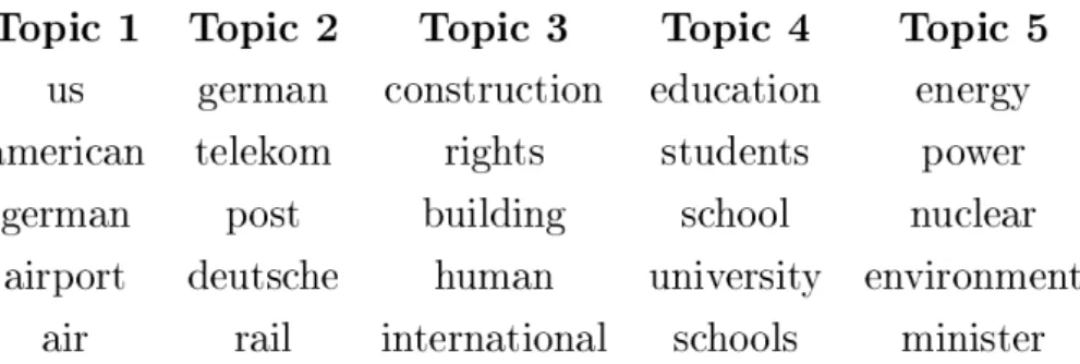
Topic models are a type of statistical model for uncovering the hidden topic structure in a collection of documents [Ble12]. By analyzing patterns of word co-occurrence, topic models discover a semantically meaningful structure from an unstructured document collection for further organization and exploration. Since topic modeling does not require extra labels of the data, it can be easily applied to a large collection of data which is quite common in the information age. Probabilistic latent seman-tic indexing (PLSI) is an early and classic topic model proposed in 1999 [Hof99]. Later, a Bayesian extension of PLSI was proposed known as Latent Dirichlet Alloca-tion (LDA) [BNJ03], which soon became prevalent in both industry and academia because it generalizes better to unseen data. When applying LDA to text data, our main target is to estimate two sets of parameters: (1) topic distributions of documents, which measure the similarities between documents; (2) word distribu-tions of topics, which represent the topic structure learned from the data. Figure 1 shows ve topics of a LDA model trained on De-News data, each of which lists top 5 words with the highest probability. It is not dicult for us to infer the con-tent of each topic based on its top words, which veries the eectiveness of LDA. Currently, LDA is a cornerstone of many topic model extensions, such as temporal LDA [WAB12, DBJ12], correlated topic models [BlL06], regularized topic models [PSC10, NBB11] and supervised topic models [BlM07].

The world is becoming more and more closely connected with the development of the Internet. Consequently, the ability of accessing documents in dierent languages has been in an increasing demand by the Internet users. Multilingual LDA (MLDA) models are proposed to address the topic modeling problem in a multilingual set-ting, which are usually variants of LDA. There are two types of MLDA, the ones that assume parallelism of the training corpus [NSH09, MWN09, DeM09] and the ones that do not [BoB09, JaD10]. In this thesis, we focus on MLDA with parallel data because it does not require extra linguistic resources, such as translators or multilingual dictionaries. Moreover, the popularity of Wikipedia makes it easy to get parallel corpora in various languages. In the rest of the thesis, we will refer to MLDA with parallel data as simply MLDA.

Parallel corpora can be further classied into two types: sentence-aligned parallel corpora and document-aligned parallel corpora (also known as comparable parallel corpora). A sentence-aligned parallel corpus contains direct translations of each document in several languages, while a document-aligned corpus contains

(6)

topic-Figure 1: Five selected topics of a LDA model trained on De-News data, each of which lists top 5 words with the highest probability.

aligned documents in several languages instead of direct translations. Due to the parallelism assumption of MLDA, a sentence-aligned parallel corpus is more ideal than a document-aligned corpus because the former guarantees each document tuple in dierent languages has the same topic distribution. However, to create such ne corpus is time-consuming and labor-intensive. Moreover, the size of sentence-aligned corpus is usually small, which may aect the generalization of an MLDA model. Alternatively, document-aligned parallel corpora are abundant and easy to access, such as Wikipedia. A drawback of such corpora is that it does not strictly follow the parallelism assumption, which may aect the performance of MLDA to some extent.

Gibbs sampling and variational inference are two popular algorithms for training LDA [Hei04, BlL09], and they can be adopted to MLDA naturally [NSH09, VDT, DeM09]. However, due to the special structure of MLDA, both algorithms become bulky and inecient. More specically, the training time of MLDA increases lin-early with the number of languages under the standard framework, which can be unbearable when the data is big or there are many languages.

To address the problem mentioned above, we propose an approximate training framework of MLDA. The proposed framework aims to reduce the training time of MLDA by approximating the topic distributions of documents with only the data from one language. By doing this, documents in dierent languages can be trained separately rather than jointly. When the training of the rst language is nished, the documents of the remaining languages only need to estimate the word distributions of the corresponding languages so that the training time is reduced. We validate the performance of the proposed MLDA training framework with both Gibbs sampling and variational inference, where the experimental data covers the two types of par-allel corpora, two pairs of languages and dierent sizes of data (see more details in

(7)

Section 5.2).

The rest of the thesis is organized as follows. Section 2 introduces some background information on LDA and its training algorithms. Section 3 presents MLDA model as well as its training algorithms. Section 4 describes the proposed approximate training framework of MLDA and its adoption with Gibbs sampling and variational inference. The experimental settings and results analysis are presented in Section 5. Section 6 draws a conclusion of the thesis.

2 Background Knowledge

In this chapter, we will rst introduce the categorical and Dirichlet distributions as a preliminary. After that, we introduce LDA model, which is built upon the two distributions. Then we present two training algorithms of LDA, namely Gibbs sam-pling and variational inference. We also give running examples of the two training algorithms, respectively. At last, we briey discuss the similarities and dierences between Gibbs sampling and variational inference.

2.1 Categorical and Dirichlet Distributions

Categorical distribution and Dirichlet distribution are two distributions used in LDA. In this subsection, we will briey introduce the properties of the two dis-tributions so that some of the calculations can be simplied later.

The categorical distribution describes the probability of a random event that hasK

possible outcomes. Its probability mass function is

p(z =i|θ) = θi, (1)

where z is a categorical random variable, and θ is a K-dimensional parameter.

The Dirichlet distribution is the conjugate prior of the categorical distribution, which guarantees that the posterior distribution has the same form as the prior. Its prob-ability density function is

p(θ|α) = Γ( PK i=1αi) QK i=1Γ(αi) K Y i=1 θαi_i −1, (2)

(8)

where θ is a Dirichlet random variable, and α is a K-dimensional parameter.

The expectation of the Dirichlet distribution oni-th dimension can be calculated as

follows E[θi|α] = αi PK i=1αi . (3)

Assuming that n outcomes of θ are observed and denoted by z, we can derive the

posterior of θ as follows p(θ|z, α)∝p(θ, z|α) =p(θ|α) n Y j=1 p(zj|θ) = Γ( PK i=1αi) QK i=1Γ(αi) K Y i=1 θ_iαi−1 n Y j=1 θzj = Γ( PK i=1αi) QK i=1Γ(αi) K Y i=1 θ_iαi−1+ni, (4)

where ni is the number of zj = i. We see that the posterior has the same form as the Dirichlet, so we can get its expectation on i-th dimension using Formula 3:

E[θi|z, α] =

αi+ni

PK

i=1αi+n

. (5)

We will also need the log expectation of the Dirichlet on i-th dimension, which can

be calculated as the following equation:

E[logθi|α] = Ψ(αi)−Ψ( K

X

i=1

αi), (6)

where Ψ(·) is known as digamma function.

2.2 Latent Dirichlet Allocation (LDA)

LDA is a probabilistic generative model, which aims to nd the latent structure of a given data in an unsupervised way. Although LDA has been largely used on text

(9)

data, it can also be used on various other data sources, such as image data [WBF09] and genome data [PLM10].

In terms of text modeling, LDA assumes that each document has a distribution over topics, where each topic is a distribution over all the words. After training with a given text data, LDA estimates the topic distribution of each document as well as the word distribution of each topic. These discovered topic distributions help us explore the homogeneity and heterogeneity of a given set of documents on a thematic level. On the other hand, the estimated topic structure (i.e. word distributions) tells us the meaning of each topic in an easily comprehensible manner.

As a generative model, LDA can be described as a generative process, which gives an intuitive description of the connection between the model and the data. We describe the generative process of LDA as follows:

for all topics k ∈[1, K] do

Draw βk∼DirV(η); // Dir denotes Dirichlet distribution end

for all documents d∈[1, D] do

Draw θd∼DirK(α);

for all words n∈[1, Nd] do

Draw zd,n∼Cat(θd); // Cat denotes categorical distribution Draw wd,n ∼Cat(βzd,n);

end end

Algorithm 1: Generative process of LDA.

From the generative process, we can see that each word distribution βk is a random variable that follows a V-dimensional Dirichlet distribution, where V is the size of

the vocabulary. Similarly, each topic distribution θd is a K-dimensional Dirichlet random variable, where K is the number of topics. We usually call βk and θd parameters because they are the unknown variables that we are interested in. In Bayesian statistics, parameters are further parameterized by hyperparameters so that full Bayesian inference is possible. In this case, βk and θd are parameterized by η and α, respectively. As the parameters of Dirichlet distributions, η and α

are supposed to be vectors. Since we use symmetric Dirichlet here so that all the dimensions of its parameter are equal, η and α will be scalars in this thesis. The

(10)

the topic distribution θd of its corresponding document. After the latent topic is decided, the wordwd,nis then drawn as a categorical random variable parameterized by the word distribution of its latent topic. In the following text, we use a single letter to denote the collection of the same type variables. For example, θ denotes

all the topic distributions, while θd denotes the one of the d-th document.

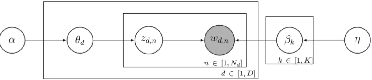
LDA can also be seen as a directed graphical model, which is a special case of graphical models. Graphical models simplify inference computations by assuming conditional independence between random variables. A graphical model representa-tion of LDA is shown in Figure 2.

α θd zd,n wd,n βk η

n ∈ [1, Nd] d∈ [1, D]

k ∈ [1, K]

Figure 2: Graphical model of LDA. The unshaded nodes are hidden random vari-ables, while the shaded one is an observed random variable. The directed edges illustrate the dependencies between random variables. The boxes denote replica-tions of the random variables. θd is a random variable of topic distribution for document d, parameterized by α. βk is a random variable of word distribution for topick, parameterized byη. wd,n is an observed variable that denotes then-th word of document d, whilezd,n is its latent topic which is unobserved.

In contrast to the frequentist, Bayesian statistics treats parameters as random vari-ables. Thus, Bayesian methds maintain a probability distribution of all the hidden variables (including parameters) by constantly incorporating observations into the model. When no observation is observed, the distribution of the parameters is called the prior, which is set manually. After incorporating observations, the distri-bution becomes the posteriorp(z|x, α), wherez denotes hidden variables, xdenotes

observed variables, and α is hyperparameters. So training an LDA model is to

compute its posterior distribution with a given data and hyperparameters:

(11)

We see that the denominator in Formula 7 is actually the integral of the numerator, and this posterior has been shown to be intractable to compute because of the in-tegral [BNJ03]. Consequently, we will need approximate algorithms to compute the posterior. Gibbs sampling and variational inference are two widely used approxi-mate algorithms of LDA. Since computing the posterior is the key of LDA, we will introduce the two algorithms as well as their advantages and disadvantages in the rest of the chapter.

2.3 Gibbs Sampling

2.3.1 Overview

Gibbs sampling is a Markov Chain Monte Carlo (MCMC) technique, which attempts to approximate the target distribution by collecting samples from it [ReH09]. More specically, an MCMC technique draws samples sequentially by constructing a rst-order Markov Chain of samples. The main dierence between dierent MCMC techniques is the choice of transition probabilities from one sample to another. As for Gibbs sampling, it draws the next sample by successively updating the state of each dimension of the current sample. In other words, we update one dimension of the current sample by xing its other dimensions, which can be done by sampling from the conditional distribution of the current dimension given the other dimensions. 2.3.2 Gibbs Sampling for LDA

From the description of Section 2.3.1, we get an idea that the most essential part of deriving a Gibbs sampler for a specic model is to derive its conditional distributions of hidden variables. As the conditional distributions are proportional to the joint distribution, we rst write down the joint distribution of LDA:

(12)

p(zd,n=k|z¬(d,n), θ, β, w, α, η) = p(zd,n =k|θd, wd,n, β, α, η)

∝p(zd,n=k|θd)p(wd,n|βk)

=θd,kβk,wd,n,

(9)

wherez¬(d,n)denotes all the latent topics except forzd,n, and the rule applies to other

variables similarly. By using the conditional independence of graphical models, we can see that the derivation is largely simplied.

The conditional distribution of a topic distribution can be derived using Formula 4:

p(θd|z, θ¬d, w, β, α, η) =p(θd|zd, α)

=Dir(α+nd),

(10)

where nd is a K-dimensional count of hidden topic assignments. The conditional of the word distribution is analogous

p(βk|z, θ, w, β¬k, α, η) = p(βk|z, w, η)

=Dir(η+mk),

(11)

where mk is a V-dimensional count of word occurrences in topic k.

Collapsed Gibbs sampling is a better Gibbs sampling algorithm that integrates out all the hidden variables except for z [Gri02, GrS04]. By doing this, the sampling

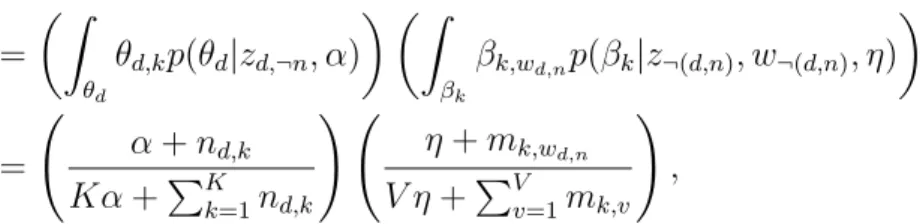
space becomes smaller, thus the sampler converges faster. Using collapsed Gibbs sampling, we only need to derive the conditional distribution of zd,n by integrating out the parameters θ and β:

(13)

= Z θd θd,kp(θd|zd,¬n, α) Z βk βk,wd,np(βk|z¬(d,n), w¬(d,n), η) = α+nd,k Kα+PK k=1nd,k ! η+mk,wd,n V η+PV v=1mk,v ! ,

where z¬(d,n) denotes all the latent topics except for zd,n, and zd,¬n denotes all the latent topics in document d except for zd,n. The rule also applies to w analogously.

Note that the counts nd,k and mk,v have excluded zd,n and wd,n.

The collapsed Gibbs sampler can be initialized by randomly assigning topics to each

zd,n. After certain iterations of sampling, the sampler converges, and the last sample

is used to estimate the expectation of the posterior distribution of parametersθand β as follows: ¯ θd,k = α+nd,k Kα+PK k=1nd,k , (13) and ¯ βk,v = η+mk,v V η+PV v=1mk,v . (14)

Algorithm 2 gives the collapsed Gibbs sampling algorithm for LDA. 2.3.3 A Running Example

We give a simple example to illustrate how LDA discovers topic structures in a given data set with collapsed Gibbs sampling. This toy data contains three documents, denoted as d1, d2 and d3. Document d1 has three dierent words

{education, student, school}, where each word is repeated 10times. Similarly,

doc-ument d2 has three words {energy, power, nuclear}, and document d3 has words

{construction, building, worker}, both with 10repetitions.

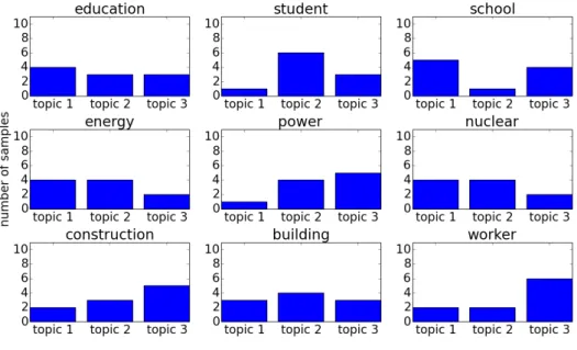
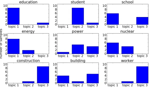
Before training, each word in each document will be assigned a topic randomly. Figure 3 shows the statistics of the initial topic assignments. There are nine bar graphs for nine dierent words, and the words in the same row are from the same document. We can see that most words do not have strong bias towards a specic topic because the topic assignments are random.

(14)

Data: D documents

Result: expected topic distributions _θ¯_{and expected word distributions} _β¯

initialize the topic of each word with random assignment; while not reach iteration number ITER_NUM1 do

for all words n∈[1, Nd] do for all topics k∈[1, K] do

calculate unnormalized probability of topic k using Formula 12;

end

normalize the above topic distribution;

sample a topic from the topic distribution and assign it to the current word;

end end end

calculate _θ¯_{with statistics from the latest topic assignment using Formula 13;}

calculate _β¯ _{with statistics from the latest topic assignment using Formula 14;}

Algorithm 2: Collapsed Gibbs sampling for LDA.

Figure 3: Statistics of topic assignments before training with collapsed Gibbs sam-pling.

(15)

Figure 4 shows the statistics of topic assignments after one training iteration with collapsed Gibbs sampling. Some words start to bias a specic topic, which will lead to more biased topic distributions later. Intuitively, this kind of convergence is based on word co-occurrence. When two words co-occur in the same document, they are cosidered to be similar in terms of topics.

Figure 4: Statistics of topic assignments after one training iteration with collapsed Gibbs sampling.

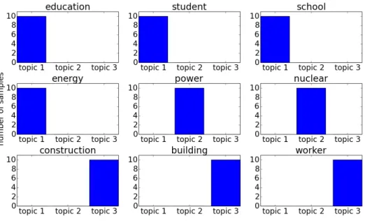
Figures 5-7 show the topic statistics after 8, 10 and 12 training iterations,

respec-tively. From Figure 7, we can see that the assigned topics are biased in a regular way, which indicates that the algorithm has converged. The words from d1, d2 and

d3 are assigned to topic 1, 2 and 3, respectively. Then, we use these topic samples

to estimate expected topic distributions _θ¯_{and expected word distributions} _β¯_with

Formulas 13 and 14. Tables 1 and 2 show the estimated _θ¯ _and _β¯ _{with collapsed}

(16)

Figure 5: Statistics of topic assignments after eight training iterations with collapsed Gibbs sampling.

Figure 6: Statistics of topic assignments after 10 training iterations with collapsed

(17)

Figure 7: Statistics of topic assignments after 12 training iterations with collapsed

Gibbs sampling. The algorithm has converged.

Topic1 Topic2 Topic3 Doc1 0.996 0.002 0.002 Doc2 0.002 0.996 0.002 Doc3 0.002 0.002 0.996

Table 1: Expected topic distributions _θ¯_{estimated with collapsed Gibbs sampling.}

Each row is a normalized probability distribution that sums to one.

2.4 Variational Inference

2.4.1 Overview

Unlike Gibbs sampling, variational inference transforms an inference problem into an optimization problem [Bea04]. To be more specic, variational inference uses a simpler distribution of the hidden variables q(z|ν) to approximate the true but

intractable posterior distribution p(z|x, α). The parameters ν is usually called

vari-ational parameters. By optimizing the varivari-ational parameters, varivari-ational inference nds the best combination that gives the closest approximate distribution to the true posterior.

(18)

Topic1 Topic2 Topic3 education 0.327 0.003 0.003 student 0.327 0.003 0.003 school 0.327 0.003 0.003 energy 0.003 0.327 0.003 power 0.003 0.327 0.003 nuclear 0.003 0.327 0.003 construction 0.003 0.003 0.327 building 0.003 0.003 0.327 worker 0.003 0.003 0.327

Table 2: Expected word distributions _β¯ _{estimated with collapsed Gibbs sampling.}

Each column is a normalized probability distribution that sums to one.

Kullback-Leibler(KL) divergence is often used to measure the closeness of two dis-tributions. Its denition on q(z|ν) and p(z|x, α)is

KL(q(z|ν)||p(z|x, α)) =Eq log q(z|ν) p(z|x, α) . (15)

So the optimization problem of variational inference is to minimize the KL divergence by optimizing ν. Unfortunately, we cannot optimize the KL divergence directly

because we do not know p(z|x, α). Thanks to Jensen's inequality, it can be shown

that the log probability of the observed variables is actually bounded:

The last term is usually called evidence lower bound (ELBO) because it is a lower bound of logp(x|α), which is known as evidence. By further expanding Formula 15,

(19)

KL(q(z|ν)||p(z|x, α)) =Eq log q(z|ν) p(z|x, α) =Eq[logq(z|ν)]−Eq[logp(z|x, α)]

(17)

So the KL divergence is actually the sum of the negative ELBO and the evidence. Because the evidence does not depend onq(z|ν), maximizing the ELBO is equivalent

to minimizing the KL divergence. Intuitively, when the ELBO nds its maximum, which is equal to logp(x|α), the KL divergence becomes zero, and it indicates that

we have found the true posterior. However, we are usually not able to nd the true posterior because the approximate posterior is a simplied posterior that ignores certain properties.

Before we actually optimize the ELBO, we need to decide which family of distri-butions q(z|ν) is in so that it will be easy to compute its expectations. Mean-eld

variational distributions are frequently used in this case [BNJ03, BlL09] because they are exible and they have no extra assumptions oven hidden variables except for their independence. That is to say, the hidden variables become independent from each other:

q(z|ν) =

m

Y

j=1

q(zj|νj), (18)

where m denotes the number of hidden variables.

With the independence assumption, we can simplify the ELBO as follows:

In this thesis, we will use coordinate ascent algorithm to optimize the ELBO, how-ever, there are many other more advanced optimization techniques, such as natural

(20)

gradient [HRK10, KRH09] and conjugate gradient [HRL12]. Coordinate ascent op-timizes one variational parameter at a time by xing the others. By doing this, it optimizes each variational parameter iteratively until it converges to a local opti-mum. To apply coordinate ascent, we need to calculate the subpart of the ELBO that is related to the current variable we are optimizing. By seeing the current variable as the last variable in the chain rule in Formula 19, we get:

ELBOj =E[logp(zj|z¬j, x, α)]−Ej[logq(zj|νj)] +const

= Z q(zj|νj)E¬j[logp(zj|z¬j, x, α)]dzj− Z q(zj|νj)logq(zj|νj)dzj. (20)

By taking the derivative of ELBOj with respect to q(zj|νj), and making it zero, we get the update equation of the variational parameterνj:

q∗(zj|νj)∝exp{E¬j[logp(zj|z¬j, x, α)]}. (21) If the conditional probability in Formula 21 is in the exponential family, the update equation can be further simplied [Bea04, XJR03, BlJ05]:

ν_j∗ =E[η(z¬j, x, α)], (22)

where η(z¬j, x, α) denotes the natural parameter of the conditional probability in the exponential family distributions.

2.4.2 Variational Inference for LDA

Applying the mean-eld theory to LDA gives us a variational distribution of LDA:

q(β, θ, z|ν) = K Y k=1 q(βk|λk) D Y d=1 q(θd|γd) Nd Y n=1 q(zn|φd,n) ! , (23)

where λ, γ and φ are variational parameters of β, θ and z, respectively. We will

then derive the update equations for the three variational parameters.

As for βk, its conditional distribution (Formula 11) is just Dirichlet distribution,

which is in the exponential family. We then substitute Formula 11 into Formula 22 to get the update equation ofλk,v:

(21)

λk,v=η+ D X d=1 Nd X n=1 1(wd,n=v)φn,k. (24) Similarly, we can substitude Formula 10 into Formula 22 to get the update ofγd,k:

γd,k=α+ Nd

X

n=1

φd,n,k. (25)

Because the conditional distribution of zd,n (Formula 9) is not in the exponential family, we substitute Formula 9 into Formula 21 to get the update ofφd,n,k:

φd,n,k ∝exp{Eγd[logθd] +Eλk[logβk,wd,n]}. (26) The log expectation of Dirichlet can be computed as digamma functions (see Formula 6), so the more detailed update is:

φd,n,k ∝exp{Ψ(γd,k)−Ψ( K X j=1 γd,j) + Ψ(λk,wd,n)−Ψ( V X v=1 λk,v)} ∝exp{Ψ(γd,k) + Ψ(λk,wd,n)−Ψ( V X v=1 λk,v)}. (27)

Because variational inference is sensitive to the initialization, we use an empirical technique to initialize λ [BlL09]. In addition to the initialization λk,v = η, we add extra counts. For each λk, we randomly select a seed document from the training

data, and add the word counts of the document toλk. As forγ, we simply initialize

it as γd,k =α+Nd/K.

After the variational inference has converged, we estimate the expectation of the posterior distribution of the parametersθ and β as follows:

¯ θd,k= γd,k PK k=1γd,k , (28) and ¯ βk,v = λk,v PV v=1λk,v . (29)

(22)

Data: D documents

initialize λ and γ;

while the ELBO not converged do for all documents d∈[1, D] do

for all words n∈[1, Nd] do for all topics k∈[1, K] do

update φd,n,k using Formula 27; end

normalize φd,n;

for all topics k∈[1, K] do

update γd,k using Formula 25; update λk,v using Formula 24; end

end end end

calculate _θ¯_{with the latest variational parameter} _γ _{using Formula 28;}

calculate _β¯ _{with the latest variational parameter} _λ _{using Formula 29;}

Algorithm 3: Variational inference for LDA. 2.4.3 A Running Example

We use the same toy data as in Section 2.3.3 to give a running example of LDA with variational inference. Recall that for each topic k, we randomly select a seed

document to initialize the value of λk. In this specic run, the seed documents for λ1, λ2 and λ3 are d3, d2 and d3, respectively.

Figure 8 shows the expected topic assignments φ after one training iteration with

variational inference. Some words become biased quickly because of the initialization with seed documents.

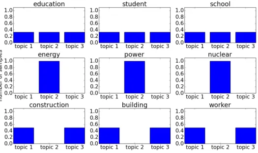
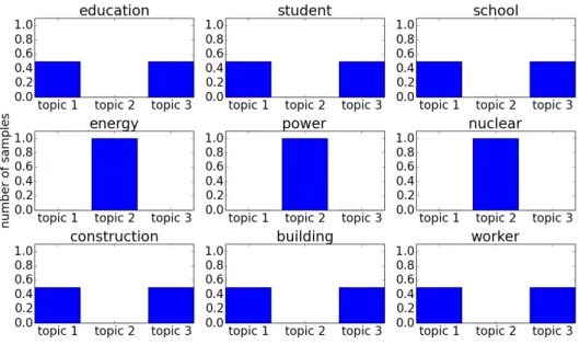
Figures 9 and 10 show the expected topic assignments after two and ve training iterations with variational inference, respectively. Figure 10 has actually converged, although the topic assignments are not good enough. This indicates that the solution from variational inference is an approximate to the true value. However, if the seed documents become d1, d2 and d3 for λ1, λ2 and λ3, the expected topic assignments

(23)

Figure 8: Expected topic assignmentsφ after one training iteration with variational

inference.

after convergence will be just as good as that of collapsed Gibbs sampling. So initialization is important to the performance of variational inference.

Figure 9: Expected topic assignmentsφafter two training iterations with variational

(24)

Figure 10: Expected topic assignments φ after ve training iterations with

varia-tional inference. The algorithm has converged.

After convergence, we use the latest variational parameters γ and λ to estimate

expected topic distributions _θ¯ _{and word distributions} _β¯ _{with Formula 28 and 29.}

Tables 3 and 4 show the values of the estimated _θ¯_and _β¯_.

Topic1 Topic2 Topic3 Doc1 0.498 0.004 0.498 Doc2 0.003 0.994 0.003 Doc3 0.498 0.004 0.498

Table 3: Expected topic distributions _θ¯_{estimated with variational inference. Each}

row is a normalized probability distribution that sums to one.

2.5 Gibbs Sampling vs Variational Inference

By observing that the update equation of variational inference (Formula 21) is also based on full conditional distributions of the hidden variables, we see a close con-nection between variational inference and Gibbs sampling. The dierence between the two is that Gibbs sampling is a sampling-based algorithm, while variational in-ference is a deterministic algorithm based on optimization. In general, variational

(25)

Topic1 Topic2 Topic3 education 0.165 0.003 0.165 student 0.165 0.003 0.165 school 0.165 0.003 0.165 energy 0.003 0.327 0.003 power 0.003 0.327 0.003 nuclear 0.003 0.327 0.003 construction 0.165 0.003 0.165 building 0.165 0.003 0.165 worker 0.165 0.003 0.165

Table 4: Expected word distributions _β¯ _{estimated with variational inference. Each}

column is a normalized probability distribution that sums to one.

inference converges faster but the result is biased. On the contrary, Gibbs sampling usually converges slower but the result is unbiased.

In terms of LDA, we can use collapsed Gibbs sampling instead of the standard one, which gives a faster and unbiased result. It has been shown that collapsed Gibbs sampling gives a comparable computational eciency to variational inference and it has a better model accuracy [AWS09]. Despite the inferior performance on LDA, variational inference possesses the potential scalability to large data, which we will discuss in Section 5.6.

3 Multilingual LDA (MLDA)

3.1 Model Description

Through the Internet, the world is closely connected, and all the digital documents should be easily accessible to each user. However, in the context of multilingual topic modeling, standard topic models become inappropriate. To address this prob-lem, a multilingual extension of LDA has been proposed due to the eectiveness and prevalence of LDA. We call this extension MLDA, which usually falls into two categories: (1) MLDA with parallel corpus [NSH09, MWN09, DeM09]; (2) MLDA without parallel corpus [BoB09, JaD10]. We focus on the former one in this thesis because it does not require extra linguistic resources, thus it is more concise and lighter. However, if necessary, extra lexicon can also be merged into the model to

(26)

improve the performance [VDM13].

MLDA is built upon LDA, with only a little modication: it assumes a parallel cor-pus in L languages, where each group of a language is modeled as an LDA model.

Additionally, the topic distribution of each document is shared across dierent lan-guages, while the topic structures (i.e. word distributions) of dierent languages are independent of each other. Due to this simple yet essential assumption, the words in dierent languages with similar topics are aligned so that the topic structures of dierent languages are aligned. When there are new documents in dierent lan-guages to be inferred, they can be transformed into the same latent semantic vector space for comparison.

We describe the generative process of MLDA as follows: for all languages l∈[1, L]do

for all topics k ∈[1, K] do

Draw β_k(l)∼DirV(l)(η(l));

end end

Draw θd∼DirK(α);

for all languages l∈[1, L]do

for all words n∈[1, N_d(l)] do

Draw z_d,n(l) ∼Cat(θd); Draw w_d,n(l) ∼Cat(β(l) z(_d,nl)); end end end

Algorithm 4: Generative process of MLDA.

The graphical model of MLDA is also similar to LDA, shown in Figure 11. It can be roughly seen as a combination of L LDA models, where L is the number

of languages. An essential component that links these single LDA models is the topic distribution variable θd, which is shared across languages. For convenience

and simplicity, we assume η(l) ₌ _η _{for all the languages in the rest of the thesis}

so that the hyperparameters are still scalars. The training of MLDA can also be accomplished by either Gibbs sampling or variational inference. We will give more

(27)

details of the two algorithms with MLDA in the rest of the chapter. α θd z_d,n(2) w(2)_d,n β_k(2) η(2) z_d,n(1) w(1)_d,n β_k(1) η(1) z_d,n(L) w_d,n(L) β_k(L) η(L) .. . .. . .. . n∈ [1, N_d(1)] l= 1 n∈ [1, N_d(2)] l= 2 n ∈ [1, N_d(L)] l=L k ∈ [1, K] k ∈ [1, K] k ∈ [1, K] m ∈ [1, M]

Figure 11: Graphical model of MLDA. The unshaded nodes are hidden random variables, while the shaded one is an observed random variable. The directed edges illustrate the dependencies between random variables. The boxes denote replications of the random variables. θd is a random variable of topic distribution for document

d, shared across languages. αis the hyperparameter of θd. For each language, there

is a random variableβ_k(l)that denotes word distribution for topick, wherek ∈[1, K].

η(l) is the hyperparameter of β_k(l). For the same document, each language also has

its own observed word variablewd,n and the corresponding latent topic zd,n.

3.2 Gibbs Sampling for MLDA

We derive the collapsed Gibbs sampler of MLDA as follows:

p(z_d,n(l) =k|z_¬¬₍(_d,nl) ₎, w, α, η) ∝p(z_d,n(l) =k, w(_d,nl)|z_¬¬₍(l_d,n) ₎, w_¬¬(₍l_d,n) ₎, α, η) ∝ Z βk Z θd p(θd, β (l) k , z (l) d,n=k, w (l) d,n|z ¬(l) ¬(d,n), w ¬(l) ¬(d,n), α, η) (30)

(28)

= βk θd p(z_d,n(l) =k, w_d,n(l)|θd, βk)p(θd|z ¬(l) d,¬n, α)p(β (l) k |z (l) ¬(d,n), w (l) ¬(d,n), η) = Z βk Z θd θd,kβ (l) k,wd,np(θd|z ¬(l) d,¬n, α)p(β (l) k |z (l) ¬(d,n), w (l) ¬(d,n), η) = Z θd θd,kp(θd|z ¬(l) d,¬n, α) Z βk β_k,wd,n(l) p(β_k(l)|z_¬(l₍)_d,n₎, w_¬(l₍)_d,n₎, η) = α+ PL l=1n (l) d,k Kα+PL l=1 PK k=1n (l) d,k ! η+m(_k,wl) d,n V η+PV v=1m (l) k,v ! ,

where z_¬¬₍(_d,nl) ₎ denotes all the topic assignments in all the languages except for z_d,n(l),

andz_d,¬(_¬l)_n denotes all the topic assignments of documentdin all the languages except

for z_d,n(l). The counts here n(_d,kl) and m_k,v(l) have also excluded z_d,n(l) and w_d,n(l).

After the sampler converges, the expectation of the posterior distribution of param-eters θ and β can be calculated as follows:

¯ θd,k = α+PL l=1n (l) d,k Kα+PL l=1 PK k=1n (l) d,k , (31) and ¯ β_k,v(l) = η+m (l) k,wd,n V η+PV v=1m (l) k,v . (32)

Algorithm 5 gives the collapsed Gibbs sampling algorithm for MLDA.

3.3 Variational Inference for MLDA

It is also straightforward to extend variational inference from LDA to MLDA. We rst give the update equation of λ(k,v:l)

λ(_k,vl) =η+ D X d=1 Nd X n=1 1(w(_d,nl) =v)φ(_n,kl). (33)

Similarly, the update equation of γd,k is:

γd,k =α+ L X l=1 Nd X n=1 φ(_d,n,kl) . (34)

(29)

Data: D documents in Llanguages

initialize the topic of each word with random assignment; while not reach iteration number ITER_NUM1 do

end

normalize the topic distribution;

end end end end

calculate _β¯ _{with statistics from the latest topic assignment using Formula 32;}

Algorithm 5: Collapsed Gibbs sampling for MLDA.

φ(_d,n,kl) ∝exp{Eγ_d[logθd] +E_λ(l)

k

[logβ(l)

k,w(_d,nl)]}. (35) By substituting digamma functions into Formula 35, we further get:

φ(_d,n,kl) ∝exp{Ψ(γd,k)−Ψ( K X j=1 γd,j) + Ψ(λ (l) k,wd,n)−Ψ( V X v=1 λ(_k,vl))} ∝exp{Ψ(γd,k) + Ψ(λ (l) k,wd,n)−Ψ( V X v=1 λ(_k,vl))}. (36)

The initialization here is analogous to that of LDA. Note that the selected seed document of eachλk is now shared across languages so that they have similar initial topic structures. After the variational inference has converged, we estimate the expectation of the posterior distribution of the parameters θ and β as follows:

(30)

¯ θd,k= γd,k PK k=1γd,k , (37) and ¯ β_k,v(l) = λ (l) k,v PV v=1λ (l) k,v . (38)

Algorithm 6 gives the variational inference algorithm for MLDA. Data: D documents in Llanguages

while the ELBO not converged do for all languages l∈[1, L]do

update φ(_d,n,kl) using Formula 36;

end

normalize φ(_d,nl);

update γd,k using Formula 34; update λ(_k,vl) using Formula 33;

end end end end end

(31)

4 Proposed Approximate Training Framework

In this section, we propose an approximate training framework for MLDA. The new framework aims to reduce the training time of MLDA by estimating parameters of dierent languages separately and approximating the topic distributions with latent topics from only one language. The framework works with both Gibbs sampling and variational inference.

4.1 Framework Description

Nowadays, with fast growing data, computational eciency becomes an essential criterion for an algorithm in addition to accuracy. In other words, an optimal objective of an algorithm is to nd the best trade-o between eciency and accuracy. In this context, an algorithm that gives the best accuracy with a poor eciency still has room for improvement. The current training framework of MLDA is a framework with such potential ineciency. For both Gibbs sampling and variational inference, the training time of MLDA is L times as long as that of LDA because there are L copies of each document in dierent languages in MLDA. Such a long training

time is unbearable in practice, especially when the data is large or there are many languages. We argue that the topic distributions θ can be approximated by using

latent topic variables from one language rather than all the languages. By doing this, it is possible to train documents in dierent languages separately. Since θ can

be estimated with documents from just one language, the restL−1sets of parallel

documents can just x the known θ and use it directly. Notice that theseL−1sets

of parallel documents will need much fewer training iterations to converge because

β is the only parameter to estimate whileθis known. This is similar to the inference

stage whereβ is known but θ is to be estimated.

4.2 Approximate Gibbs Sampling for MLDA

Under the new framework, collapsed Gibbs sampler will rst estimate the shared parameter θ and a private parameter β of a language. For convenience, we denote

the rst trained language as language 1 and the rest as languages 2 to L. More

specically, we rst do collapsed Gibbs sampling for the documents in language 1

(32)

p(z(1)_d,n=k|z¬_¬₍(1)_d,n₎, w, α, η) = α+L·n (1) d,k Kα+PK k=1L·n (1) d,k ! η+m(1)_k,wd,n V η+PV v=1m (1) k,v ! , (39)

where the counts n(1)_d,k and m(1)_k,v have excluded z_d,n(1) and w(1)_d,n. Note that in Formula

39, we add a multiplier L for each statistics n(1)_d,k to make its scale consistent with

the original sampler.

Then, _θ¯_and _β¯(1) _{can be estimated using the following formula after it converges:}

¯ θd,k = α+L·n(1)_d,k Kα+PK k=1L·n (1) d,k , (40) and ¯ β_k,v(1) = η+m (1) k,wd,n V η+PV v=1m (1) k,v . (41)

When doing sampling for language 1, we know little about the topic distrbutions, so we initialize the topic of each word randomly. Now that we getθ after training

lan-guage 1, we can do better than random initialization on lanlan-guages2toL. However,

it is still not possible to know which word is correlated to which topic in languages

2 toL because they have dierent vocabularies from language1. Alternatively, we

can initialize the topic of each word in a document as the one with the largest topic probability in this document. More specically, we initialize each topic as follows:

z(_d,nl) = arg max

k∈[1,K]

θd,k, (42)

where l ranges from 2 to L. We call this empirical technique Greedy Initialization

(GI).

We then do collapsed Gibbs sampling for languages 2 to L using the following

formula: p(z(_d,nl) =k|z¬_¬₍(_d,nl) ₎, w, α, η) = α+L·n (1) d,k Kα+PK k=1L·n (1) d,k ! η+m(_k,wd,nl) V η+PV v=1m (l) k,v ! . (43)

(33)

Finally, we estimate _β¯(2) _to_β_¯(L) _{as follows:} ¯ β_k,v(l) = η+m (l) k,wd,n V η+PV v=1m (l) k,v . (44)

Algorithm 7 gives the approximate collapsed Gibbs sampling algorithm for MLDA.

4.3 Approximate Variational Inference for MLDA

Following the same approximate framework as in Section 4.2, we will rst train on language 1 using variational inference. We give the update equation of λ(1)_k,v as

follows: λ(1)_k,v=η+ D X d=1 Nd X n=1 1(w(1)_d,n=v)φ(1)_n,k. (45)

Then, we update the shared variational parameterγd,k:

γd,k =α+L· Nd

X

n=1

φ(1)_d,n,k, (46)

where Lis a multiplier to keep its scale the same as the standard algorithm.

The update equation of φ(1)_d,n,k is:

φ(1)_d,n,k ∝exp{Eγd[logθd] +E_λ(1)

k

[logβ(1)

k,w(1)_d,n]}. (47) By substituting digamma functions into Formula 47, we further get:

φ(1)_d,n,k ∝exp{Ψ(γd,k)−Ψ( K X j=1 γd,j) + Ψ(λ (1) k,wd,n)−Ψ( V X v=1 λ(1)_k,v)} ∝exp{Ψ(γd,k) + Ψ(λ (1) k,wd,n)−Ψ( V X v=1 λ(1)_k,v)}. (48)

(34)

initialize the topic of each word in language 1 with random assignment; while not reach iteration number ITER_NUM1 do

for all documents d∈[1, D] of language 1 do

for all words n∈[1, N_d(1)] do

end

end end end

calculate _β¯(1) _{with statistics from the latest topic assignment using Formula 41;}

use greedy initialization for documents in language l, wherel ∈[2, L];

while not reach iteration number ITER_NUM2 do for all documents d∈[1, D] of language l do

end

end end end

calculate _β¯(l) _{with statistics from the latest topic assignment using Formula 44;}

end

(35)

After language 1, we update λ(l) and φ(l) for languages 2to L: λ(_k,vl) =η+ D X d=1 Nd X n=1 1(w(_d,nl) =v)φ(_n,kl), (49) and

φ(_d,n,kl) ∝exp{Eγd[logθd] +E_λ(l)

k

[logβ(l)

k,w(_d,nl)]}. (50) By substituting digamma functions into Formula 50, we further get:

φ(_d,n,kl) ∝exp{Ψ(γd,k)−Ψ( K X j=1 γd,j) + Ψ(λ(_k,wd,nl) )−Ψ( V X v=1 λ(_k,vl))} ∝exp{Ψ(γd,k) + Ψ(λ (l) k,wd,n)−Ψ( V X v=1 λ(_k,vl))}, (51)

where γ is taken from Formula 46, and xed in Formula 51.

The initialization remains the same as in section 3.3. Unlike approximate collapsed Gibbs sampling in Section 4.2, we do not have greedy initialization here for languages

2 to L because they are already initialized with seed documents (see more details

in Section 3.3). The estimates of _θ¯_and _β¯ _{are also the same as the standard model}

(see Formula 37 and 38).

Algorithm 8 gives the approximate variational inference for MLDA.

5 Experiments

We design a crosslingual documents matching task to test the performance of the proposed approximate training framework of MLDA, and compare it with the stan-dard framework. Because it is sucient to demonstrate the performance of the new framework with a bilingual model, we use bilingual parallel corpus in all the experi-ments. The rst set of experiments are based on sentence-aligned parallel corpus of English-German, while the second ones are based on comparable parallel corpus of English-Chinese.

(36)

while the ELBO not converged do

for all documents d∈[1, D] of language 1 do

for all words n∈[1, N_d(1)] do

update φ(1)_d,n,k using Formula 48;

end

normalize φ(1)_d,n;

update γd,k using Formula 46; update λ(1)_k,v using Formula 45;

end end end end

while the ELBO not converged do for all languages l∈[2, L]do

for all documents d∈[1, D] of language l do

update φ(_d,n,kl) using Formula 51;

end

normalize φ(_d,nl);

update λ(_k,vl) using Formula 49;

end end end end end

(37)

5.1 The Matching Task

After we train the MLDA model on a parallel corpus, we get estimates ofβ(l)for each

language. Then, we are able to infer the topic distribution θ(l) of a new document

in any language l that among languages 1 to L. If the new document has been

written in languages 1 to L, the trained MLDA is supposed to assign similar topic

distributions to the same document in dierent languages. Crosslingual documents matching is a task that reects such ability of an MLDA model.

We use Euclidean distance to measure the distance between two expected topic distributionsθ1 and θ2: d(θ1, θ2) = v u u t K X k=1 (θ1,k −θ2,k)2, (52) where k denotes the topic index.

The matching task evaluates model accuracy by the average neighbor gap between expected topic distributions of two languages in the test data with the following formula: Average_Neighbor_Gap= 1 M M X m=1 Neighbor_Gap(θ_m(1), θ(2)), (53)

where M is the number of documents in the test data, θ(1)m denotes the expected topic distribution of the m-th document in language 1 in the test data, and θ(2)

denotes the expected topic distributions of all the documents in language 2 in the test data. The function Neighbor_Gap(θ(1)m , θ(2))returns the ranking of θ(2)m among

θ(2) toθm(1) based on Euclidean distance in ascending order. A lower value of average neighbor gap indicates a better MLDA model.

5.2 Dataset

5.2.1 De-News

De-News is an English-German parallel corpus1_{, in which documents are collected}

from the daily news of German radio broadcast from August 1996 to January 2000.

(38)

After removing incomplete documents, it contains 9667 pairs of English-German

parallel documents, with each sentence aligned to its counterpart. To use it as an input to MLDA, we remove non-alphabet characters and stopwords for each language. After preprocessing, there are on average 61 tokens for each English

document and57tokens for German. We use the rst9000 pairs to estimate model

parameters and the rest667 pairs for performance evaluation.

5.2.2 Wikipedia

The Wikipedia Comparable Corpora2 _{provides bilingual document-aligned corpora}

on tens of language pairs. Unlike sentence-aligned texts, document-aligned texts are aligned on the topic level rather than direct translations. The corpus we use in this experiment is part of the Wikipedia Comparable Corpora on English-Chinese language pair, which contains 55000 pairs of documents. These documents are

selected with comparable document length to avoid document pairs with extreme imbalance. As a preprocessing step, we remove meaningless characters, stopwords and low-frequency words with occurrence less than ve for both languages. For the Chinese corpus, we additionally do traditional-to-simplied Chinese transformation and words segmentation. After preprocessing, there are on average 202 tokens for

each English document and 213 tokens for Chinese. The rst 50000 pairs are used

to estimate model parameters and the rest 5000 pairs are for performance test.

5.3 Results on De-News Data

5.3.1 Approximate Gibbs Sampling

In this experiment, we set the number of topics of MLDA as 50. Since we use

symmetric Dirichlet distributions as priors, the hyperparameter α is all set to 1

(calculated by an empirical formula 50/K [GrS04], where K is the number of

top-ics), and η is all set to 0.1. For the approximate Gibbs sampler, we do 100 Gibbs

sampling iterations for language 1 (English) and {1,2,3,4,5,10,20,50,100}

itera-tions for language2(German). For the standard Gibbs sampler, the Gibbs sampling

iteration number is100for both languages. We use100because it is where the

stan-dard algorithm starts to converge. In order to verify the eectiveness of GI, we also add an approximate Gibbs sampler without GI. After parameter estimation, we do

(39)

inference on the expected topic distributions _θ¯_{of the test data with the estimated} ¯

β. The sampling iteration number of inference is 20. Finally, the accuracy of the

model is evaluated with average neighbor gap using the expected topic distributions of the test data. Each recorded model accuracy is an average of 10 runnings with

dierent random seeds.

Figure 12 shows the results of the three samplers in this experiment. After100

iter-ations of training on two languages, the model with standard Gibbs sampler reaches

10.087average neighbor gap on the test data. As for the approximate Gibbs sampler

without GI, its average neighbor gap decreases quickly as the iteration number on language 2 grows. And it starts to converge after about 10 iterations on language 2 with 11.879 average neighbor gap. Through using GI, the approximate Gibbs

sampler converges even faster, at about 5 iterations with 12.110 average neighbor

gap. Therefore, GI is an eective method for reducing training time in MLDA with the approximate Gibbs sampler.

Figure 12: Results of the standard Gibbs sampler and the faster Gibbs sampler (with and without GI) on the original De-News English-German corpus. Note that the x-axis denotes the training iterations on language 2, so the average neighbor

gap of the standard algorithm is xed because its has a xed number of training iterations on language2.

Although the approximate Gibbs sampler saves 95 sampling iterations (47.5% of

(40)

the standard Gibbs sampler on model accuracy. This gap indicates the approxima-tion of topic distribuapproxima-tion_θ¯_{in approximate Gibbs sampler is not close enough to the}

one in standard algorithm. To be more specic, the samples (latent topics) in only language 1 is not sucient to give an estimate ofθ¯that approximates the estimate

from samples in both language 1 and 2. We will do further empirical experiments

to see how the number of samples aects the accuracy of distribution estimation. In order to see the eect of dierent document lengths (number of samples) on the ac-curacy of distribution estimation, we conduct a simple and empirical experiment. In MLDA, the target value_θ¯_{is the expectation of a Dirichlet posterior. To simulate the}

inference procedure here, we dene the target value_θˆ_{as the parameter of a}

multino-mial distribution with equal probabilities in all the categories. The target value_θˆ_{is a}

K-dimensional vector (i.e. there are K categories), in which K ∈[50,100,200,400].

We then sample N samples from the multinomial distribution parameterized by

ˆ

θ, where N ∈ [30,50,75,100,125,150,175,200,300,400,500,600,700,800]. We also

see _θˆ_{as the expectation of a Dirichlet posterior with a symmetric Dirichlet prior.}

We dene the hyperparameter α as 50/K, where K is the number of topics. To

estimate the target _θˆ_{, we use the same formula as Formula 13.}

A single estimation error is calculated with the following formula:

Error(ˆθ_true,θˆ_est) = 1

K K X k=1 (ˆθ_truek −θˆk_est)2, (54) where_θˆ

true is the true distribution,θˆest is the estimate, andk denotes an index of a

vector. In order to reduce the variance of the error, we take an average of 50 trials

for each recorded error.

Figure 13 shows the estimation error with dierent number of topicsK and samples N. We see that the empirical results are very similar in the four settings with

dier-ent number of topics, so the number of topics is not an essdier-ential factor that aects the accuracy of the estimation. In terms of a specic topic number K, the

estima-tion error drops quickly in the beginning as the number of samples increases. Then the rate of decrease becomes small after about 200 samples, and it is approaching

zero after 500 samples. From the empirical results, we can get a rough idea that

if the average document length is over 500 in MLDA model, then the estimate of ¯

θ from using documents in one language will be very close to the one from using

documents in all the languages. For the experiment above, the average document length is around 60, which has a signicant gap to 120 (number of samples from

(41)

documents in two languages) on estimation error.

Figure 13: Empirical results about the eect of dierent document lengths on dis-tribution estimation accuracy.

Based on the above empirical results, an ideal average document length is over500

for the approximate Gibbs sampler of MLDA. But in practice, we can loosen the restriction to around 200, which also gives a reasonable estimate of the true value.

In the next extra experiment, we simply triple each document of De-News, with now the average length of English corpus being 183 and that of German being171. The

other experimental settings all remain the same as the rst experiment in Section 5.3.1.

Figure 14 shows the results of the Gibbs samplers on triple-length De-News corpus. The average neighbor gap of standard Gibbs sampler is 4.276. The approximate

Gibbs sampler without GI converges at 20 iterations with 4.311 average neighbor

gap. Again, GI helps speed up the convergence of the approximate Gibbs sampler, and it converges at15iterations with4.349average neighbor gap. Most importantly,

the approximate Gibbs sampler now gets a close accuracy to the standard algorithm, which veries the results of the empirical experiment in return.

(42)

Figure 14: Results of the standard Gibbs sampler and the approximate Gibbs sam-pler (with and without GI) on the triple-length De-News English-German corpus. Note that the x-axis denotes the training iterations on language 2, so the average

neighbor gap of the standard algorithm is xed because its has a xed number of training iterations on language 2.

Because the approximate Gibbs sampler simplies the sampling formulas, it also reduces computation time per iteration compared to the standard algorithm. Table 5 gives the computation time of training the two samplers. We can see that the training time of two languages per iteration is reduced to5.481 seconds from 6.948

seconds by the approximate Gibbs sampler. Additionally, the approximate algorithm signicantly reduces sampling iterations on language2. Hence, we conclude that the

approximate Gibbs sampler saves48.9% training time with almost no loss on model

accuracy on triple-length De-News data.

Language Time per iteration Iterations Total time Standard Gibbs Two Languages 6.948 sec 100 694.80 sec

Faster Gibbs Language 1 3.211 sec 100 355.15 sec

Language 2 2.270 sec 15

Table 5: Training time of standard and approximate Gibbs sampler on triple-length De-News.

(43)

5.3.2 Approximate Variational Inference

For variational inference, the topic number and hyperparameters remain the same as in Section 5.3.1. As for the approximate variational inference, we do70iterations

for language 1 (English) and {1,2,3,4,5,10,20,50,70} iterations for language 2

(German). We do 70 iterations for both languages for the standard variational

inference because it converges after70. In order to make the result comparable with

Gibbs sampling, we evaluate the model accuracy on the test data using the standard collapsed Gibbs sampling, which is the same as in Section 5.3.1. Variational inference is a deterministic algorithm, and it converges to a local optimum, which makes it sensitive to the initialization. Hence, we choose the best model from ve dierent random seeds on initialization instead of doing the average.

Figure 15 shows the result of the experiment. The standard variational inference has 11.294 average neighbor gap on the test data, while the approximate algorithm

reaches 11.352 after it converges at 20 iterations on language 2. So the

approxi-mate variational inference gets a comparable accuracy to the standard model on the matching task, and meanwhile it saves 50 iterations of training on language 2. In

contrast to Gibbs sampling, there is almost no accuracy gap between approximate variational inference and its standard algorithm on the original De-News data. This is because variational inference estimates with expectations instead of sampling. When using the expectations of the latent topics to estimate a topic distribution, two or more copies of the same document (but in dierent languages) do not increase the accuracy of the estimate theoretically. That is to say, under ideal circumstances, using documents from only one language rather than all languages does not aect the performance on estimating topic distributions for variational inference. In practice, such property holds to some extent but not strictly.

Table 6 shows the training time in this experiment. Under the approximate frame-work, variational inference saves about 38.1% training time compared to the

(44)

Figure 15: Result of the standard variational inference and the approximate vari-ational inference on the De-News English-German corpus. Note that the x-axis

denotes the training iterations on language 2, so the average neighbor gap of the

standard algorithm is xed because its has a xed number of training iterations on language 2.

Language Time per iteration Iterations Total time Standard VI Two Languages 7.02 sec 70 491.4 sec

Faster VI Language 1 3.327 sec 70 304.09 sec

Table 6: Training time of standard and approximate variational inference on original De-News data.

5.4 Results on Wikipedia Data

5.4.1 Approximate Gibbs Sampling

Because the data here is larger, we set the number of topics as 100. The

hyperpa-rameterα is all set to0.5(calculated by the empirical formula50/K [GrS04], where K is the number of topics), and η is all set to 0.1. For the standard Gibbs

sam-pler, the Gibbs sampling iteration number is 500 for both two languages, where the

(45)

sampling iterations for language 1 (English) and {1,5,10,20,30,40,100,300,500}

iterations for language 2 (Chinese). We also test the approximate Gibbs sampler

without GI in this experiment. The inference settings and the evaluation metric remain the same as in Section 5.3.1.

Figure 16 shows the result of the experiment. Similar to Figure 14, the approximate Gibbs sampler with and without GI converges at around 20 and 30 iterations,

re-spectively, both of which reach very close model accuracy to that of the standard sampler. Therefore, approximate Gibbs sampling also works well on comparable parallel data.

Figure 16: Result of standard Gibbs sampler and approximate Gibbs sampler (with and without GI) on the Wikipedia English-Chinese corpus. Note that the x-axis

From the training time of the samplers showed in Table 7, we see that the approxi-mate Gibbs sampler saves56.2% training time compared to the standard algorithm.

Compared to the one in Section 5.3.1, the approximate algorithm in this experiment is more time-ecient because the necessary sampling iterations of the standard al-gorithm are many more, while only a few more iterations are needed on language 2

(46)

Language Time per iteration Iterations Total time Standard Gibbs Two Languages 88.737 sec 500 44368.5 sec Faster Gibbs Language 1 37.629 sec 500 19446.2 sec

Table 7: Training time of the standard and the approximate Gibbs sampler on Wikipedia English-Chinese corpus.

5.4.2 Approximate Variational Inference

In this experiment, the topic number and hyperparameters are the same as in Sec-tion 5.4.1. The standard variaSec-tional inference converges after 200 iterations on the

Wikipedia corpus, so we test the performance of the standard algorithm at iteration

200. For the approximate algorithm, we do 200 iterations for language 1 (English)

and {1,3,5,10,20,30,50,100,200} iterations for language2(Chinese). The

remain-ing settremain-ings are the same as in Section 5.3.2.

Figure 17 shows the result of the experiment. The standard variatioanl inference gets 204.69 average neighbor gap when it converges. The approximate algorithm

converges at about20-th iteration on language 2with 283.43average neighbor gap.

As we can see from the gure, the model accuracy of the approximate algorithm is much worse than that of the standard algorithm, which does not occur in the ex-periments on De-News data with variational inference. Compared to the De-News data, the Wikipedia data has about 5times as many documents and twice as many

topic dimensions, so there are about10times as many topic distribution parameters

in the Wikipedia data. From the previous discussions, we already know that varia-tional inference is quite sensitive to the initializations because it converges to a local optimum deterministically. Therefore, we suspect that the much larger parameter space makes it even more sensitive to the initializations. If the initialization is not good, the approximate variational inference may converge to a bad local optimum for language 1, which means the estimate of the topic distributions is poor. Then,

the estimate of the word distributions of language 2 might not be aligned well to

that of language 1 because of the poor estimate. Additionally, the topic

distribu-tions in the Wikipedia data are not aligned as well as in De-News data, which may also aect the performance of the approximate algorithm.

(47)

Figure 17: Result of the standard variational inference and the approximate vari-ational inference on the Wikipedia English-Chinese corpus. Note that the x-axis

In order to validate our speculation preliminarily, we do an extra experiment. We simply reduce the topic number to 20 to narrow the parameter space. We keep the

other settings the same as above except that the number of iterations of convergence becomes 150. Figure 18 gives a comparison of the two results with dierent topic

numbers, both of which are the best among ve dierent random seeds. We can see that the accuracy gap between the standard and approximate algorithm is signi-cantly reduced when the topic number becomes20, which conrms our speculation

above. However, the performance of variational inference is still much worse than that of collapsed Gibbs sampling on the Wikipedia data. To further validate the performance of approximate variational infernce on MLDA with large data, better inference methods and more advanced optimization techniques are required, which will be left as a future plan (see Section 5.6 for more details).

To see the eciency improvement that approximate variational inference gets com-pared to Gibbs sampling, we record its training time on the Wikipedia data with100

topics. From Table 8, we can see that approximate variational inference saves about

(48)

is not satisfactory enough.

Figure 18: Performance comparison of variational inference with dierent topic num-bers on the Wikipedia English-Chinese corpus. Note that the x-axis denotes the

training iterations on language 2, so the average neighbor gap of the standard

al-gorithm is xed because its has a xed number of training iterations on language

2.

Language Time per iteration Iterations Total time Standard VI Two Languages 188.265 sec 200 37652.9 sec Faster VI Language 1 109.418 sec 200 23570.1 sec

Table 8: Training time of standard and approximate variational inference on Wikipedia English-Chinese corpus.

5.5 Comparison of the Two Algorithms

According to the experimental results, we nd that standard collapsed Gibbs sam-pling outperforms variational inference on accuracy in the MLDA model while their eciency are comparable, which is consistent with the results from other papers [AWS09]. When the proposed approximate framework is applied, collapsed Gibbs