Using floorplans for software visualization

(1)

Using floorplans for software visualization

∗ Z. Apanovich, M. Bulyonkov, A. Bulyonkova

P. Emelyanov, N. Filatkina, P. Ruyssen

Abstract. In this article we consider requirements to visualization of semantic properties of programs appearing in the reengineering process when use of hierar-chical ordering is an appropriate way to visualize the information of interest. We consider two algorithms of graph placement that implement geometrical inclusion of object hierarchy. They use (non)slicing floorplan techniques that is being actively developed in VLSI design domain. Some illustrating examples are given.

Introduction

Maintenance of complex legacy software is a well-known hard problem that requires a lot of resources. Any activity in this area, such as reengineering, refactoring, or retargeting, begins with code analysis and understanding. Roughly speaking, it consists of the following basic steps:

1) identify objects of interest;

2) attribute the objects with appropriate information; 3) detect relationships between the objects;

4) identify sub-systems of the entire system in order to enforce divide-and-conquer approach.

All this knowledge should be stored in some sort of repository, that provides model-based access to object information. The precision of the analysis may depend on the overall objectives and/or computational resources.

Program reengineering most often is partially automated and requires user interaction [19]. Therefore there should be some means to visualize the information from the repository. Naturally, objects and relationships can be represented in a form of a graph [12]. There exist many both common-purpose and specialized graph drawing packages for software visualization [2, 8]. The graph layout methods that are used in these packages may be categorized as follows:

1) algorithms of tree visualization [14];

∗ _{This work was supported by the Russian Foundation for Basic Researches under}

(2)

tionships to be analyzed. Recently developed hierarchical methods of graph layout and visualization seem to open a promising way to the solution of this problem.

The rest of the paper is organized as follows: in the first section we briefly consider graph editor BEDit which is currently used in our reengi-neering system1. Next we discuss some issues that need to be addressed for visualization of hierarchical relationships. Finally we consider two algo-rithms of graph layout that realize hierarchy as geometrical inclusion. They use both slicing and non-slicing floorplans techniques that are actively used in VLSI design. Some illustrating examples are given.

1. BEDit

Although the textual representation of the source code is its dominating representation, there are a number of cases when graphical representations may make it more understandable. Among typical examples are flowcharts, call graphs, etc. The BEDit graph editor was implemented for visualization of objects and relationships. Some textual information can be associated with them.

The following criteria were taken into consideration for the choice of the placement algorithms:

1. In the context of reverse engineering graphs help the user in compre-hension of the source code structure. Hence one of the most important criteria for evaluation of the quality of visualization is readability of representation. Recent research has shown that the main factor which influences the readability of representation is the number of edge cross-ings [16].

2. Usually the source code is maintained and modified, and graphs are generated on user demand. For this reason, graphs should be gener-ated rapidly, in order to reduce the user waiting. The requirement of interactivity imposes serious restrictions on algorithm efficiency. So, our attention should be primarily paid to the time consumed by layout algorithms.

(3)

3. There is no need to provide stability of visualization: minor changes in the source code may lead to generation of a completely different representation.

Basically a link between two objects is represented by an edge connecting corresponding boxes. The input format of BEDit is xml-based and looks as follows:

The algorithm [18] was adapted to be used in the reengineering environ-ment. A new algorithm realizing a kind of layered drawing was developed for layout of mostly acyclic graphs.

The algorithm consists of the following steps:

1) identification of an acyclic graph, distribution of nodes by levels, and detection of the base trees;

2) layout of spanning trees and sorting of nodes at the same level; 3) reduction of the occupied space and correction of placement of nodes

at each level;

4) correction of the placement to fit box sizes; 5) layout of edges.

Our algorithm pays more attention to the initial placement of the span-ning tree than the classical algorithms do. This allows us to reduce in ad-vance the number of edge crossings and hence to reduce the time consumed by the following phases of the algorithm.

Sorting of nodes at each level is done by the barycentric method [7]. The initial tree layout, together with sorting of nodes, is a good approximation to the desired result and significantly improves convergence of the iterative barycentric process.

When the placement and sizes of nodes are fixed, we minimize the num-ber of edge crossings. Since we consider only the orthogonal edges, the problem can be reduced to the graph coloring problem. This problem is

(4)

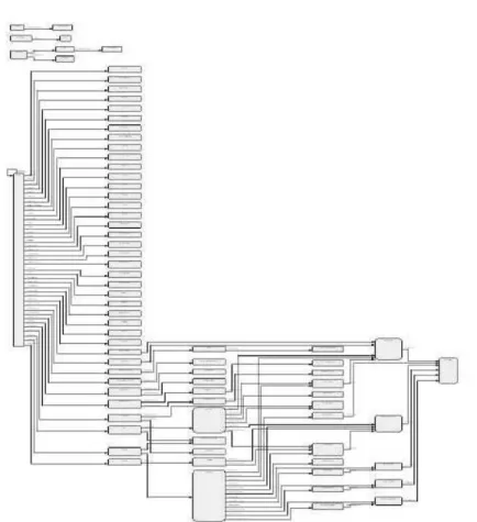
Figure 1. Visualization in BEDit graph editor

NP-complete and we used a heuristic algorithm [4]. An example of using of BEDit that shows dependencies among program modules of a legacy system is given on Figure 1.

2. The use of geometrical-inclusion representations in program understanding

In the process of program understanding [5], we consider a program as a col-lection of related entities that have appropriate attributes. This is similar to the usage of the well-known model of entity-relationship diagrams (ERD). The model was adapted for the visualization purposes in the following way: 1. The relationship of nesting was introduced. It reflects the syntactical

hierarchy of program constructs.

2. The formal model was enriched with a textual representation of objects so that the objects of the model become attached to the syntactical constructs that represent the objects.

(5)

3. The model was extended to provide for the abstract types and inher-itance mechanism. This allows for definition of type hierarchy. For instance, the “statement” type may have descendants types “condi-tional statement”, “assignment statement”, etc. which inherit state-ment’s attributes and relationships.

We used the geometrical-inclusion representations in the form of floor-plans (see the definition in Section 3). Before their description, we give some examples arising in reengineering and program understanding.

2.1. Syntactical nesting

First of all, floorplans may be used to represent the syntactical construct nesting. Usually the tree-like representation is used for this purpose: a program is presented as a set of trees, each root corresponding to a module or file, which constitute the program. Although such representation may have a considerably lower level of details as compared to the full abstract syntax tree, it still may be over-detailed. So in some cases it may be useful to restrict the set of displayed types, for example, to display only calls, conditionals and procedures.

In this case, the use of a floorplan instead of a tree-like representation may result in a more compact general view of a program. For example,

1. Synchronization of this representation with the source code may ease the location of the search construct.

2. The color of conditionals may vary depending on the number and depth of nested conditionals. That may give the average and maximum estimates of the program complexity.

3. A similar coloring of floorplans allows visual estimation of other mea-surable characteristics, such as the frequency of certain variables in different procedures, or location of input/output operations, etc. 2.2. Data visualization

One of the most frequently investigated program objects are data and their declarations [6, 9]. In this case the tree-like representation reflects the data type rather than data organization. Even not considering dynamically allo-cated data, pointers, etc., one may find examples where the data declaration structure differs from their physical allocation. The constructs likeunionin C, REDEFINE in COBOL, etc., impose different types on the same memory location. When this feature is used not for realization of different logical variants, but for different access to the same memory location, the user needs to know the exact allocation scheme. Here, the exact correspondence of data element sizes to visual representation sizes may be unnecessary and

(6)

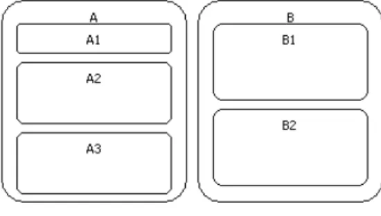
Figure 2. HyperCode. Allocation of data structures with the use ofREDEFINES mechanism

even undesirable. More important is a clear presentation of the mutual lo-cation of data elements: for example, one element is an exact subelement of another, or they have exactly the same location, or they intersect.

In the COBOL language, there are several sources of dependencies be-tween variables. First of all, this is the mechanism of REDEFINES which allows us to overlay several data structures with different names (see Fig-ure 2). In case of such overlay, i.e. when the structFig-ure A is declared as A REDEFINES B, any modification of a field of one structure implicitly changes some field of the other one. Moreover, since both the size and the structure ofAandBmay differ, an assignment to a single field ofAmay affect several fields ofB. The dependencies between variables fromAandBare determined based on the intersection of the corresponding memory locations.

In the case of statically allocated memory, it would be natural to repre-sent the inclusion relationship using the floorplan, and theA REDEFINES B relationship — by edges over it. The second kind of relationships may also be reflected by positioning of boxes in the floorplan: alternatives should be displayed in parallel, side by side.

Another source of data flow are COMPUTE and MOVE statements. They differ in the sort of induced dependencies between the arguments and the result. If complex data structures appear on both sides of the assignment, theCOMPUTEstatement implies dependence of every part of the result on the whole argument, whileMOVE statement dependencies are similar to those of REDEFINES.

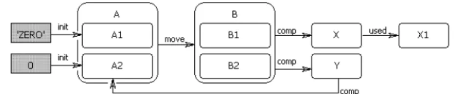
Arbitrary complexity of data structures and partial overlay during eval-uation of dependencies lead to the conclusion that the basic items for the description of data flow should be all elementary memory locations produced by the intersection of overlayed data elements, rather than the syntactical concept of “variable” (see Figure 3). Nevertheless, for proper comprehension of such data flow representation, the user should be able to easily obtain in-formation about the origin of a particular location with appropriate reference to the source code.

(7)

Figure 3. HyperCode. Representation of the data flow of structured data

So, in this case, we also have two types of relationships: nesting and data dependencies. A floorplan is used to display the hierarchical data structure, and the data flow is shown as links between the most nested boxes corresponding to elementary fields.

2.3. Control visualization

The control structure of a program is a traditional candidate for being rep-resented in the graphical form. Obviously, in this case the graphical repre-sentation is one of the most easily understandable. However, it also has a number of technical and methodological difficulties.

First of all, it requires more space than, say, the textual representation. The whole graph of a real program most probably won’t fit the screen size with sufficient details, so the user will have to scroll it back and forth with-out any guarantee of seeing the interesting parts of the graph all at once. Another problem is that the control flow graph for real programs may be very cumbersome and require complex layout algorithms, which may not be acceptable because of the interactive character of visualization. A com-promise between the response time and quality of visualization should be found.

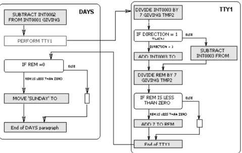
A significant simplification of the call graph may be achieved by intro-duction of a graph hierarchy. The natural two-level hierarchy for COBOL is a separate representation of the paragraph call graph (HCCallie) and con-trol inside paragraph (HCParagraph). Following this approach, the user can see all details of control without losing the overall picture. Moreover, construction of the intra-paragraph control may be more efficient and simple due to better structuring (see Figure 4).

More generally, simplification of the graphical representation of the con-trol flow may be achieved by using floorplans for inclusion of procedures and separate control graph for each procedure (see Figure 5).

(8)

Figure 4. HyperCode. Intra-paragraph control flow graph

(9)

Figure 6. HyperCode. Procedure call graph

2.4. Inter-program visualization

We have already mentioned that analysis of program components is only the beginning of understanding of a program system. At the next stage, the data and control flow between program modules should be understood. The preparation of information for visualization is essentially very similar to the process of linking separately compiled modules. Modules may be of different nature: programs, database table definitions, description of screen forms, etc. An important requirement is that information be collected and placed into the repository incrementally, while modules are analyzed one by one. The possibility to view and analyze incomplete information is even more important because quite often the system are either incomplete or not closed, since they may use system or third party components which are unavailable in the reengineering environment.

One should also keep in mind that, in general, the static program analysis can give only approximation of data flow. This happens, in particular, when SQL queries or screen forms are generated dynamically depending on the values of program variables. In such cases the system may require information from the user.

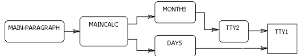
The user should have a possibility to change the level of consideration: from the analysis of interaction of program components to their internal structure, and, after navigation inside a program, back to the upper level, perhaps in a different place. In other words, it should be possible to hide certain levels of a floorplan and to lift relationships to the parents, and to promptly return the hidden when necessary. For example, on Figure 6 we see a call graph, and on the next picture (Figure 7) — the same graph and the content of the paragraph TTY1, preserving the general call context.

A similar approach can be used for the data flow, as well (see Figure 8). The grouping based on programs and procedures provides a natural hierar-chy. Floorplans, together with the possibility to collapse boxes, significantly simplify the process of exploration of data flow by hiding the details which are not relevant to the current program.

(10)

Figure 7. HyperCode. Joint representation of procedural calls and internal procedure control

Figure 8. HyperCode. Inter-program data flow

3. Floorplans

A relationship between objects may be represented not only by edges but also by nesting of boxes. Figure 2 shows visualization of the contains– relationship: an arc between two boxes means that the second object is a part of the first one.

At the first step to representation of the same relationship by geometrical nesting, each node of the graph which has outgoing arcs becomes a group of related nodes. If a node has more than one incoming arc (i.e., the object belongs to several groups), it is copied — one copy per each incoming arc. As a result we obtain the nesting tree, and edges of this type are no longer explicitly specified in the xml-representation:

(11)

</group> </groups> </graph>

Now we need to find an optimal placement of elements of each group in the hierarchy such that the boxes should not overlap, the occupied space should be minimal, and the resulting rectangle should have the required proportions. This is a typical problem of the rectangle packing and its NP-completeness is proven, for example, in [3]. This problem was actively studied in the recent years in the context of VLSI design and is known as the problem of an optimal floorplan.

Our first layout algorithm is based on the model of so-called slicing floor-plans described for the first time in [15]. This model treats the nesting tree as a scheme which determines the order of assembling rectangular elements with a specified height and width pair by pair. We used the algorithm gen-erating a solution that does not require an iterative procedure improving its quality for the reasons of efficiency. The heuristics consisted in bottom-up traversal of the nesting tree in an attempt to generate a layout for each group independently with a minimal size and its aspect ratio close to 1.

The kernel of the algorithm is the procedure of placement of a set of rectangles. Since the sizes of the elements of the group are already known, we can sort them descending the maximal size of each rectangle, and then add them one by one to the placement.

At each step of the placement, the set of so-called control points is main-tained. We try to place the next rectangle at each of the control points in two orientations — vertical and horizontal — and so to find an optimal placement. If the next rectangle is finally placed at the control pointA, it is replaced with two new control pointsBandCwith the following coordinates:

xB = xA + w(R); yB = yA;

xC = xA;

yC = yA + h(R);

wherexA , yA, xB , yB , xC, and yCare the coordinates of control points andw(R)andh(R)are the width and height of the next rectangle according to the selected orientation.

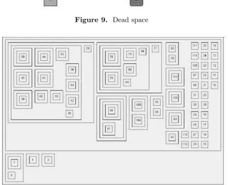
When two blocks of different sizes are assembled, a new block that con-tains both of them appears, and some space is left unoccupied (Figure 9). Such space is calleddead space. The result of the algorithm applied to data from Figure 1 is shown on Figure 10.

(12)

Figure 9. Dead space

Figure 10. The result of the algorithm

Theoretically the complexity of the algorithm is O(n2_{), where} _n _{is the} number of boxes. In practice the algorithm works fairly fast even for large samples, and can be used for interactive systems. The main flaw of this algorithm is a considerable dead space.

In order to solve the problem, another algorithm was developed utilizing the non-slicing floorplan model. A number of papers that describe data structures for the non-slicing floorplan placement appeared recently. Here are examples of such representations:

• sequence-pair,

• bounded slice line grid,

(13)

• B∗-tree,

• graph of transitive closures (TCG),

• corner block list,

• twin binary trees, etc.

More details on these representations and the corresponding placement al-gorithms can be found in [1].

The implemented approach is based on the combinatorial search in the set of configurations (or encodings) which are defined as a representation of non-slicing floorplans. Each representation is related to the rule of place-ment for a given configuration. A configuration is said to be feasible, if there exists a placement which corresponds to the configuration. Thus each configuration specifies a solution space. A placement is rated according to the space it covers. Since the exhaustive search would take too much time, heuristic methods, like simulated annealing or genetic algorithms, are used. The following four requirements help us to perform the search in the solution space efficiently [13]:

1. The solution space that is encoded by the given representation is finite. 2. Each solution is satisfiable, i.e. there is a placement that corresponds

to the given code.

3. The placement can be done in a polynomial time.

4. The code, which is evaluated to be the best for the given solution space, corresponds to one of optimal solutions.

A representation that satisfies all the four requirements is calledP-admissible. The reason of such a variety of representations is the fact that none of them satisfies all requirements to floorplans perfectly. Taking into account the restrictions of our particular task, and especially the interactive charac-ter of visualization, the LaySeq representation of floorplans [17] was chosen. The main reason for the choice is that a floorplan for a given config-uration can be generated in a linear time. Yet another advantage of the representation is a comparatively small numberO(n!) of generated configu-rations.

Although LaySeq does not satisfy the requirement of P-admissibility, since the best solution does not guarantee an optimal placement, experi-ments show that the results obtained with this placement are quite satis-factory from the practical point of view. Thus the main components of the realized placement algorithm are the following:

• the LaySeq representation that describes an acceptable set of configu-rations and allows us to select all possible configuconfigu-rations corresponding to the given representation;

(14)

Figure 12. Example of anLB-compact packing

• the rating function for the configuration quality (the space of the place-ment in the simplest case);

• the algorithm of generation of a floorplan for a given configuration;

• the procedure of generation of new configurations;

• the function that signals to stop when the best solution is found. The genetic algorithm has been chosen to iterate over the set of config-urations. Each solution in the process of the genetic algorithm is described by LaySeq data structure, which is a list of lengthn representingn blocks in the order determined at the previous phase of the procedure Figure 11.

The scheme of constructing a layout from the given sequence LaySeq is as follows:

Step 0. Creation of upper block list that contains the blocks already placed in the order of the longest side, if the side is not completely closed by blocks placed above. Initially the list is empty.

Step 1. Placement of blocks which forms the basis of a new block. While the specified number of blocks is not placed,

1) delete the next block from LaySeq;

2) place it to the right of the last placed block, so that the placement is LB-compact;2

3) Include the block into the upper block list in the position accord-ing to the block sizes.

2_{A placement is called}_L_{-compact (}_B_{-compact) iff no block can be shifted left (down)}

when all other blocks are fixed. A placement isLB-compact if it is bothL-compact and

(15)

Step 2. Place the first blocks and then make its horizontal size the width of the whole floorplan that will be maintained by the rest of the place-ment.

Step 3. While not all blocks are placed, 1) remove the next block from LaySeq;

2) place the current block on top of one of the already placed blocks to minimize the increase of the total height of the floorplan. That guarantees B-compactness of the new placement. Update the list of upper blocks and the list of neighbors for each block. The placement in the leftmost position over the selected block provides L-compactness of the placement.

Step 4. Compute the total vertical size of the floorplan.

The genetic algorithm is controlled by the following parameters:

• the number of individual solutions in a population;

• the maximal number of generations;

• the maximal number of generations without evolution(stagnation rate);

• mutation rate of an individual solution; this parameter defines the ability of a selected individuum to mute;

• mutation rate of genes; this parameter defines mutations that will be applied to a selected individuum;

• level of reproductivity; this parameter defines the number of descen-dants that will be generated by this population.

The algorithm consists of the following steps:

Population initialization. The step of initialization is performed only once, while all the rest are iterated until the solutions found are not improved any longer or the limit on the maximum of generation is reached.

Anumber of individual solutions is generated for creation of the initial population. The number should be large enough to cover most of solution space, but not excessively large for a reasonable computational time.

Selection. At each iteration the best individual solutions are selected. The number of selected solutions depends on the level of reproductivity. For example, if the level of reproductivity is 50%, then 50% of indi-vidual solutions is selected.

(16)

Layseq2 are transposed in the bounds of this subsequence. This trans-position can produce duplicate descendants in these sequences, which does not correspond to a correct solution. For example, if we trans-pose the second and third elements in the sequences Layseq1=[1,2,3,4] and Layseq2=[2,3,4,1], then new descendants become the sequences [1,3,4,4] and [2,2,3,1]. Therefore, in spite of descendants, the genera-tion correctness is checked. A modificagenera-tion is performed if needed. Mutation. Random mutations are performed to keep a genetic variety and

to avoid fast fall into a local minimum. First, by comparing the pa-rameter mutation rate of individual solution with a random value, a decision on applicability of mutation to this particular individuum is made. Next, by comparing the parametermutation rate of genes with a random value, a decision about a particular mutation is made. As mutations of individuals, the following modifications of the sequence LaySeq are used: movement of the first element of LaySeq to the end, rotation on 90o _{of one of the elements; change of BaseSizeNumber.}

The best solutions obtained by mutation are also kept.

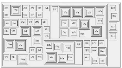
For data described above this algorithm gives the following result (Figure 13).

4. Conclusion

In this work, we consider a graph editor BEDit which is currently used in a reengineering system. We discuss the use of hierarchies in a reengineering process. Finally, we consider two algorithms of graph placement that use a geometrical inclusion of objects.

The heuristic algorithm here described has the following properties: 1. The complexity of placement for the configuration LaySeq isO(n). 2. The number of all possible configurations isO(n!).

3. The representation describes a floorplan independently from the block sizes. This allows us to use this representation for further optimiza-tions if the size of the block may vary.

(17)

Figure 13. The final result of the algorithm

4. This visualization is much better with respect to the occupied space, as compared to another one based on Sugiyama algorithm.

5. Since visualization of nesting does not exploit edges, it gives us more freedom to use edges for other relationships with less crossing.

References

[1] Apanovich Z. Tools for working with large graphs: construction and optimiza-tion of floorplans // System Informatics. — Novosibirsk: SB RAS Publisher, 2006. — Iss. 10: Methods and Models of Modern Programming. — P. 7–71. [2] Auber D. Tulip, a huge graphs visualization software // Proc. of the 9th

Internat. Sympos. Graph Drawing. — Lect. Notes Comput. Sci. — 2002. — Vol. 2265. — P. 434–435.

[3] Baker B.S., Coffman E.G., Rivest R.L. Orthogonal packings in two dimensions // SIAM J. on Computing. — 1980. — Vol. 9(4). — P. 846–855.

[4] Bulyonkova A. Approximate algorithm for large graphs coloring // Problems of Theoretical and System Programming. — Novosibirsk: Novosibirsk State University, 1982. — P. 81–86.

[5] Bulyonkov M., Baburin D., Emelianov P., Filatkina N. Visualization facilities in program reengineering // Programming and Computer Software. — 2001. — N 27(2). — P. 21–33 (Simultaneous translation from Programmirovanie). [6] Bulyonkov M., Filatkina N. Exploring data flow in legacy systems // Proc. of

the Second Asian Workshop on Programming Languages and Systems (APLAS 2001). — Daejeon: KAIST, 2001. — P. 61–75.

(18)

Bulletin. Ser.: Comput. Sci. — 2002. — Iss. 18. — P. 81–102.

[10] Fruchterman T., Reingold E. Graph drawing by force-directed placement // Software — Practice & Experience. — 1991. — Vol. 21(11). — P. 1129–1164. [11] Huang M., Eades P. A fully animated interactive system for clustering and navigating huge graphs // Proc. of the 6th_{Internat. Sympos. Graph Drawing.}

— Lect. Notes Comput. Sci. — 1998. — Vol. 1547. — P. 374–383.

[12] Koschke R. Software visualization for reverse engineering // Papers of Soft-ware Visualization: International Seminar. — Lect. Notes Comput. Sci. — 2002. — Vol. 2269. — P. 138–150.

[13] Murata H., Fujiyoshi K., Nakatake S., Kajitani Y. VLSI module placement based on rectangle-packing by the sequence pair // IEEE Trans. on Computer-Aided Design. — 1996. — Vol. 15. — P. 1518–1524.

[14] Mutzel P., Eades P. Graphs in software visualization // Papers of Software Visualization: International Seminar. — Lect. Notes Comput. Sci. — 2002. — Vol. 2269. — P. 285–294.

[15] Otten R.H.J.M. Automatic floorplan design // Proc. of the 19th_ACM/IEEE

Conf. on Design Automation. — Piscataway: IEEE Press, 1982. — P. 261–267. [16] Purchaise H. Which aesthetic has greatest effect on human understanding? // Proc. of the 5th _{Internat. Sympos. Graph Drawing. — Lect. Notes Comput.}

Sci. — 1997. — Vol. 1353. — P. 248–261.

[17] Sathiamoorthy S. LaySeq: A new representation for non-slicing floorplans // Proc. of the 6th_{IEEE VLSI Design and Test Workshop. — Piscataway: IEEE}

Press, 2002. — P. 317–327.

[18] Sugiyama K., Tagawa S., Toda M. Methods for visual understanding of hier-archical systems // IEEE Trans. on Systems, Man, and Cybernetics. — 1981. — Vol. SMC-11(2). — P. 109–125.

[19] Automatic Reengineering of Programs / Ed. by A. Terekhov, A. Terekhov Jr. — Saint-Petersburg: Saint-Petersburg State University, 2000.