Feature Selection for High-Dimensional Genomic Microarray Data
Eric P. Xing† [email protected]
Michael I. Jordan† ‡ [email protected]
Richard M. Karp† [email protected]
†Division of Computer Science, University of California, Berkeley, CA 94720 ‡Department of Statistics, University of California, Berkeley, CA 94720
Abstract
We report on the successful application of feature selection methods to a classifica-tion problem in molecular biology involving only 72 data points in a 7130 dimensional space. Our approach is a hybrid of filter and wrapper approaches to feature selec-tion. We make use of a sequence of simple filters, culminating in Koller and Sahami’s (1996) Markov Blanket filter, to decide on particular feature subsets for each subset cardinality. We compare between the re-sulting subset cardinalities using cross val-idation. The paper also investigates regu-larization methods as an alternative to fea-ture selection, showing that feafea-ture selec-tion methods are preferable in this prob-lem.
1. Introduction
Structural and functional data from analysis of the human genome have increased many fold in recent years, presenting enormous opportunities and chal-lenges for machine learning. In particular, gene ex-pression microarrays are a rapidly maturing technol-ogy that provide the opportunity to assay the ex-pression levels of thousands or tens of thousands of genes in a single experiment (Shalon et al., 1996). These assays provide the input to a wide variety of statistical modeling efforts, including classifica-tion, clustering, and density estimation. For exam-ple, by measuring expression levels associated with two kinds of tissue, tumor or non-tumor, one obtains labeled data sets that can be used to build diagnostic classifiers. The number of replicates in these exper-iments are often severely limited, however; indeed, in the data that we analyze here (cf. Golub, et al., 1999), there are only 72 observations of the expres-sion levels of each of 7130 genes. In this extreme of very few observations on very many features, it is natural—and perhaps essential—to investigate
fea-ture selection and regularization methods.
Feature selection methods have received much atten-tion in the classificaatten-tion literature (Kohavi & John, 1997; Langley, 1994), where two kinds of meth-ods have generally been studied—filter methods and
wrapper methods. The essential difference between
these approaches is that a wrapper method makes use of the algorithm that will be used to build the final classifier, while a filter method does not. Thus, given a classifier C, and given a set of features F, a wrapper method searches in the space of subsets of F, using cross validation to compare the perfor-mance of the trained classifierCon each tested sub-set. A filter method, on the other hand, does not make use of C, but rather attempts to find predic-tive subsets of the features by making use of simple statistics computed from the empirical distribution. An example is an algorithm that ranks features in terms of the mutual information between the fea-tures and the class label. Wrapper algorithms can perform better than filter algorithms, but they can require orders of magnitude more computation time. An additional problem with wrapper methods is that the repeated use of cross validation on a single data set can lead to uncontrolled growth in the proba-bility of finding a feature subset that performs well on the validation data by chance alone. In essence, in hypothesis spaces that are extremely large, cross validation can overfit.
While theoretical attempts to calculate complexity measures in the feature selection setting generally lead to the pessimistic conclusion that exponentially many data points are needed to provide guarantees of choosing good feature subsets, Ng has recently described a generic feature selection methodology, referred to as FS-ORDERED, that leads to more
optimistic conclusions (Ng, 1998). In Ng’s approach, cross validation is used only to compare between fea-ture subsets of different cardinality. Ng proves that this approach yields a generalization error that is upper-bounded by the logarithm of the number of
irrelevant features.
In a problem with over 7000 features, filtering meth-ods have the key advantage of significantly smaller computational complexity than wrapper methods, and for this reason these methods are the main fo-cus of this paper. Earlier papers that have ana-lyzed microarray data have also used filtering meth-ods (Golub et al., 1999; Chow et al., in press; Dudoit et al., 2000). We show, however, that it is also possible to exploit prediction-error-oriented wrapper methods in the context of a large feature space. In particular, we adopt the spirit of Ng’s
FS-ORDEREDapproach and present a specific
al-gorithmic instantiation of his general approach in which filtering methods are used to choose best sub-sets for a given cardinality. Thus we use simple fil-tering methods to carry out the major pruning of the hypothesis space, and use cross validation for final comparisons.
While feature selection methods search in the com-binatorial space of feature subsets, regularization or shrinkage methods trim the hypothesis space by constraining the magnitudes of parameters (Bishop, 1995). Consider, for example, a linear regression problem in which the parametersθi are fit by least
squares. Regularization adds a penalty term to the least squares cost function, typically either the squaredL2 norm or the L1 norm. These terms are multiplied by a parameterλ, theregularization
pa-rameter. Choosing λ by cross validation, one
ob-tains a fit in which the parameters θi are shrunk
toward zero. This approach effectively restricts the hypothesis space, providing much of the protection against overfitting that feature selection methods aim to provide.
If the goal is to obtain small feature sets for com-putational or interpretational reasons, then feature selection is an obligatory step. If the goal is to ob-tain the best predictive classifier, however, then reg-ularization methods may perform better than fea-ture selection methods. Few papers in the machine learning literature have compared these approaches directly; we propose to do so in the current paper.
2. Feature Selection
In this section we describe the feature selection methodology that we adopted. To summarize briefly, our approach proceeds in three phases. In the first phase we useunconditional univariate
mix-ture modeling to provide an initial assessment of the
viability of a filtering approach, and to provide a discretization for the second phase. In the second phase, we rank features according to an information gain measure, substantially reducing the number of features that are input to the third phase. Finally, in
the third phase we use the more computationally in-tense procedure ofMarkov blanket filteringto choose candidate feature subsets that are then passed to a classification algorithm.
2.1 Unconditional Mixture Modeling
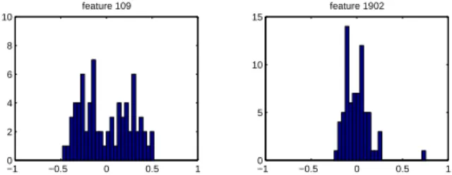
A useful empirical assumption about the activity of genes, and hence their expression, is that they generally assume two distinct biological states (ei-ther “on” or “off”). The combination of such binary patterns from multiple genes determines the sample phenotype. Given this assumption, we expect that the marginal probability of a given expression level can be modeled as a univariate mixture with two components (which includes the degenerate case of a single component). Representative samples of em-pirical marginals are shown in Figure 1.
−10 −0.5 0 0.5 1 2 4 6 8 10 feature 109 −1 −0.5 0 0.5 1 0 5 10 15 feature 1902
Figure 1.Two representative histograms of gene expres-sion measurements. The x-axes represents the normal-ized expression level.
If the underlying binary state of the gene does not vary between the two classes, then the gene is not discriminative for the classification problem and should be discarded. This suggests a heuristic pro-cedure in which we measure the separability of the mixture components as an assay of the discriminabil-ity of the feature.
Let P(fi | θi) denote a two-component Gaussian
mixture model for feature fi, whereθi denotes the
means, standard deviations and mixing proportions of the mixture model. We fit these parameters using the EM algorithm. Note that each feature fi is fit
independently.
Suppose that we denote the underlying state of gene
ias a latent variablezi∈ {0,1}. Suppose moreover
that we define a decisiond(fi) on featurefito be 0 if
the posterior probability of{zi= 0}is greater than
0.5 under the mixture model, and let d(fi) equal 1
otherwise. We now define amixture overlap
proba-bility:
=P(zi= 0)P(d(fi) = 1|zi= 0)
+ P(zi= 1)P(d(fi) = 0|zi= 1). (1)
If the mixture model were a true representation of the probability of gene expression, then the mixture
overlap probability would represent the Bayes error of classification under this model. We use this proba-bility as a heuristic surrogate for the discriminating potential of the gene, as assessed via its uncondi-tional marginal.
Note that a mixture model can also be used as a quantizer, allowing us to discretize the measure-ments for a given feature. We simply replace the continuous measurement fi with the associated
bi-nary value d(fi). This is in fact the main use that
we make of the mixture models in the remainder of the paper. In particular, in the following section we use the quantized features to define an information gain measure.
2.2 Information Gain Ranking
We now turn to methods that make use of the class labels. The goal of these methods is to find a good approximation of the conditional distribution,P(C| F), whereFis the overall feature vector andCis the class label.
Theinformation gain is commonly used as a
surro-gate for approximating a conditional distribution in the classification setting (Cover & Thomas, 1991). Let the class labels induce a reference partition
S1, . . . , SC. Let the probability of this partition be
the empirical proportions: P(T) = |T|/|S| for any subsetT. Now suppose a test on featureFi induces
a partition of the training set intoE1, . . . , EK. Let
P(Sc|Ek) =P(Sc∩Ek)/P(Ek). We define the
infor-mation gain due to this feature with respect to the reference partition as:
Igain=H(P(S1), . . . , P(SC)) − K X k=1 P(Ek)H(P(S1|Ek), . . . , P(SC|Ek)),(2)
where H is the entropy function. The information gain provides a simple initial filter with which to screen features. For example, one can rank all genes in the order of increasing information gain and select features conservatively via a statistical significance test (Ben-Dor et al., 2000).
To calculate the information gain, we need to quan-tize the values of the features. This is achieved in our approach via the unconditional mixture model quantization discussed in the previous section. 2.3 Markov Blanket Filtering
Features that pass the information gain filter are in-put to a more comin-putationally intensive subset se-lection procedure known asMarkov blanket filtering, a technique due to Koller and Sahami (1996). LetGbe a subset of the overall feature set F. Let fG denote the projection of f onto the variables in
G. Markov blanket filtering aims to minimize the discrepancy between the conditional distributions
P(C|F = f) and P(C|G= fG), as measured by a conditional entropy: ∆G= X f P(f)D(P(C|F=f)kP(C|G=fG)) where D(PkQ) = P xP(x) log(P(x)/Q(x)) is the
Kullback-Leibler divergence. The goal is to find a small feature setGfor which ∆Gis small.
Intuitively, if a feature Fi is conditionally
indepen-dent of the class label given some small subset of the other features, then we should be able to omit
Fi without compromising the accuracy of class
pre-diction. Koller and Sahami formalize this idea using the notion of a Markov blanket.
Definition 1 (Markov Blanket) For a feature
set Gand class labelC, the setMi⊆G(Fi∈/ Mi)
is a Markov BlanketofFi (Fi∈G) if
Fi⊥G−Mi− {Fi}, C | Mi
The following proposition due to Koller and Sahami establishes the relevance of the Markov blanket con-cept to the measure ∆G.
Proposition 2 For a complete feature setF, letG
be a subset of F, and G0 = G−F
i. If ∃Mi ⊆G
(where Mi is a Markov blanket of Fi), then ∆G0 =
∆G.
The proposition implies that once we find a Markov blanket of featureFiin a feature setG, we can safely
removeFifromGwithout increasing the divergence
to the desired distribution. Koller and Sahami fur-ther prove that in a sequential filtering process in which unnecessary features are removed one by one, a feature tagged as unnecessary based on the ex-istence of a Markov blanket Mi remains
unneces-sary in later stages when more features have been removed.
In most cases, however, few if any features will have a Markov blanket of limited size, and we must in-stead look for features that have an “approximate Markov blanket.” For this purpose we define
∆(Fi|M) = X
fM,fi
P(M=fM, Fi =fi)
D(P(C|M=fM, Fi=fi)kP(C|M=fM))(3).
IfMis a Markov blanket forFithen ∆(Fi|M) = 0.
Since an exact zero is unlikely to occur, we relax the condition and seek a set M such that ∆(Fi|M) is
small. Note that if M is really a Markov blanket of Fi, then we have P(C|M, Fi) = P(C|M). This
suggests an easy heuristic way to to search for a feature with an approximate Markov blanket. Since the goal is to find a small non-redundant fea-ture subset, and those feafea-tures that form an approx-imate Markov blanket of featureDi are most likely
to be more strongly correlated toFi, we construct a
candidate Markov blanket for Fi by collecting the
k features that have the highest correlations (de-fined by the Pearson correlations between the origi-nal non-quantized feature vectors) withFi, wherek
is a small integer. We have the following algorithm as proposed in (Koller & Sahami, 1996):
Initialize -G=F Iterate
- For each featureFi ∈G, letMibe the set of
k featuresFj ∈G− {Fi} for which the
cor-relations between Fi andFj are the highest.
- Compute ∆(Fi|Mi) for each i
- Choose the ithat minimizes ∆(Fi|Mi), and
defineG=G− {Fi}
This heuristic sequential method is far more effi-cient than methods that conduct an extensive com-binatorial search over subsets of the feature set. The heuristic method only requires computation of quantities of the form P(C|M = fM, Fi = fi) and
P(C|M=fM), which can be easily computed using
the discretization discussed in Section 2.1.
3. Classification Algorithms
We used a Gaussian classifier, a logistic regression classifier and a nearest neighbor classifier in our study. In this section we provide a brief description of these classifiers.
3.1 Gaussian Classifier
A Gaussian classifier is a generative classification model. The model consists of a prior probability
πc for each class c, as well as a Gaussian
class-conditional densityN(µc,Σc) for classc.1 Maximum
likelihood estimates of the parameters are readily obtained.
Restricting ourselves to binary classification, the posterior probability associated with a Gaussian classifier is the logistic function of a quadratic func-tion of the feature vector, which we denote here by
x:
P(y= 1|x, θ) = 1 1 + exp{1
2xTΛx−βTx−γ}
1Note that when the covariance matrix Σ
cis diagonal,
then the features are independent given the class and we obtain a continuous-valued analog of the popular naive Bayes classifier.
where Λ, β and γ are functions of the underlying covariances, means and class priors. If the classes have equal covariance then Λ is equal to zero and the quadratic function reduces to a linear function. 3.2 Logistic Regression
Logistic regression is the discriminative counterpart of the Gaussian classifier. Here we assume that the posterior probability is the logistic of a linear func-tion of the feature vector:
P(y= 1|x, θ) = 1 1 +e−θTx,
whereθis the parameter to be estimated. Geomet-rically, this classifier corresponds to a smooth ramp-like function increasing from zero to one around a decision hyperplane in the feature space.
Maximum likelihood estimates of the parameter vec-tor θ can be found via iterative optimization algo-rithms. Given our high-dimensional setting, and given the small number of data points, we found that stochastic gradient ascent provided an effective optimization procedure. The stochastic gradient al-gorithm takes the following simple form:
θ(t+1)=θ(t)+ρ(yn−µ(nt))xn,
whereθ(t) is the parameter vector at the tth itera-tion, whereµ(nt)≡1/(1 +e−θ
(t)T
xn), and whereρis
a step size (chosen empirically in our experiments). 3.3 K Nearest Neighbor Classification
We also used a simple K nearest neighbor classi-fication algorithm, setting K equal to three. The distance metric that we used was the Pearson corre-lation coefficient.
4. Regularization Methods
Regularization methods provide a popular strategy to cope with overfitting problems (Bishop, 1995). Letl(θ | D) represent the log likelihood associated with a probabilistic model for a data setD. Rather than simply maximizing the log likelihood, we con-sider a “penalized likelihood,” and define the follow-ing “regularized estimate” of the parameters:
ˆ
θ= arg max
θ {l(θ| D)−λkθk},
wherekθk is an appropriate norm, typically the L1 or the L2 norm, and where λ is a free parameter known as the “regularization parameter.” The basic idea is that the penalty term often leads to a sig-nificant decrease in the variance of the estimate, at the expense of a slight bias, yielding an overall de-crease in risk. One can also take a Bayesian point of
0 1000 2000 3000 4000 5000 6000 7000 8000 0 0.2 0.4 0.6 0.8 1 gene bayes error
Predictive power of the genes
0 1000 2000 3000 4000 5000 6000 7000 8000 0 0.1 0.2 0.3 0.4 0.5 0.6 0.7 gene information gain
information gain for each genes with respect to the given partition
0 50 100 150 200 250 300 350 400 0 0.05 0.1 0.15 0.2 gene K−L Divergence
K−L of each removal gene w.r.t. to its MB
(a) (b) (c)
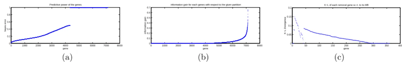
Figure 2.Feature selection using using a 3-stage procedure. (a) Genes ranked by(Eq. 1); (b) Genes ranked byIgain (Eq. 2); (c) Genes ranked by ∆(Fi|M) (Eq. 3).
view and interpret the penalty term as a log prior, in which case regularization can be viewed as a max-imum a posteriori estimation method.
The regularization parameterλ is generally set via some form of cross validation.
An L2 penalty is a rotation-invariant penalty, and shrinks the parameters along a ray toward the ori-gin. Using an L1 penalty, on the other hand, shrinks the parameters toward the L1 ball, which is not rota-tion invariant. Some of the parameters shrink more quickly than others, and indeed parameters can be set to zero in the L1 case (Tibshirani, 1995). Thus an L1 penalty has something of the flavor of a fea-ture selection method.
Parameter estimation is straightforward in the regu-larization setting, with the penalty term simply con-tributing an additive term to the gradient. For ex-ample, in the case of logistic regression with an L2 penalty, we obtain the following stochastic gradient:
θ(t+1)=θ(t)+ρ(yn−µ(nt))xn−λθ(t)
,
where the shrinkage toward the origin is apparent. In the case of Gaussian classifier, the ‘regularized’ ML estimate ofθcan be easily solved in closed form.
5. Experiments and Results
In this section, we report the results of analysis of the data from a microarray classification prob-lem. Our data is a collection of 72 samples from leukemia patients, with each sample giving the ex-pression levels of 7130 genes (Golub et al., 1999). According to pathological/histological criteria, these samples include 47 type I Leukemias (called ALL) and 25 type II Leukemias (called AML). The sam-ples are split into two sets by the provider, with 38 (ALL/AML=27/11) serving as a training set and the remaining 34 (20/14) as a test set. The goal is to learn a binary classifier (for the two cancer subtypes) based on the gene expression patterns.
5.1 Filtering Results
Figure 2(a) shows the mixture overlap probability
(defined by Eq. 1) for each single gene in ascending order. It can be seen that only a small percentage of
the genes have an overlap probability significantly smaller than 0.5, where 0.5 would constitute random guessing under a Gaussian model if the un-derlying mixture components were construed as class labels.
In Figure 2(b) we present the information gain that can be provided by each individual gene with re-spect to the reference partition (the Leukemia class labels), compared to the partition obtained from the mixture models. Only a very small fraction of the genes induce a significant information gain. We take the top 360 genes from this list and proceed with (approximate) Markov blanket filtering.
Figure 2(c) displays the values of ∆(Fi|Mi) (cf.
Eq. 3) for each Fi, an assessment of the extent
to which the approximate Markov blanketMi
sub-sumes information carried by Fi and thus renders
Fi redundant. Genes are ordered in their removal
sequence from right to left. Note that the re-dundancy measure ∆(Fi|Mi) increases until there
are fewer than 40 genes remaining. At this point ∆(Fi|Mi) decreases, presumably because of a
com-positional change in the approximate Markov blan-kets of these genes compared to the original contents before many genes were removed. The increasing trend of ∆(Fi|Mi) then resumes.
The fact that in a real biological regulatory network the fan-in and fan-out will generally be small pro-vides some justification for enforcing small Markov blankets. In any case, we have to keep the Markov blankets small to avoid fragmenting our small data set.
5.2 Classification Results
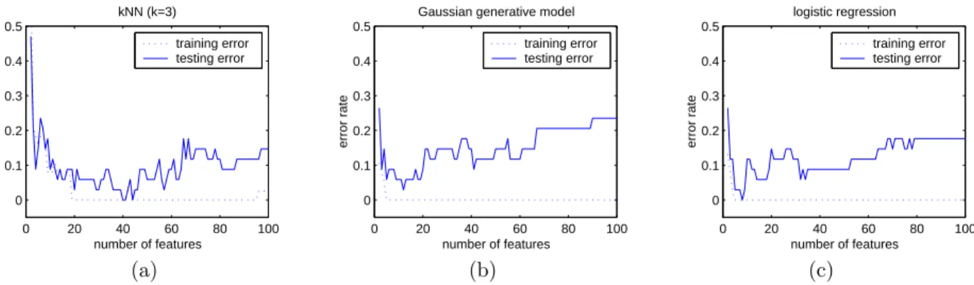
Figure 3 shows training set and test set errors for each of the three different classifiers. For each feature subset cardinality (the abscissa in these graphs), we chose a feature subset using Markov blanket filtering. This is a classifier-independent method, thus the feature subsets are the same in all three figures.
The figures show that for all classifiers, after an initial coevolving trend of the training and testing curves for low-dimensional feature spaces (the di-mensionality differs for the different classifiers), the
0 20 40 60 80 100 0 0.1 0.2 0.3 0.4 0.5 number of features error rate kNN (k=3) training error testing error 0 20 40 60 80 100 0 0.1 0.2 0.3 0.4 0.5 number of features error rate
Gaussian generative model training error testing error 0 20 40 60 80 100 0 0.1 0.2 0.3 0.4 0.5 number of features error rate logistic regression training error testing error (a) (b) (c)
Figure 3.Classification in a sequence of different feature spaces with increasing dimensionality due to inclusion of gradually less qualified features. (a) Classification usingkNN classifier; (b) Classification using a quadratic Bayesian classifier given by a Gaussian generative model; (c) A linear classifier obtained from logistic regression. All three classifiers use the same 2-100 genes selected by the three stages of feature selection.
classifiers quickly overfit the training data. For the logistic linear classifier andkNN, the test error tops out at approximately 20 percent when the entire fea-ture set of 7130 genes is used. The generative Gaus-sian quadratic classifier overfits less severely in the full feature space. For all three classifiers, the best performance is achieved only in a significantly lower dimensional feature space. Of the three classifiers,
kNN requires the most features to achieve its best performance.
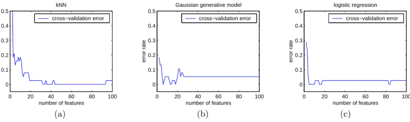
Figure 3 shows that by an optimal choice of the num-ber of features it is possible to achieve error rates of 2.9%, 0%, and 0% for the Gaussian classifier, the logistic regression classifier, and kNN, respectively. Of course, in actual diagnostic practice we do not have the test set available, so these numbers are op-timistic. To choose the number of features in an automatic way, we make use of leave-one-out cross validation on the training data. That is, for each cardinality of feature subset, given the feature sub-set chosen by our filtering method, we choose among cardinalities by cross validation. Thus we have in essence a hybrid of a filter method and a wrapper method—the filter method is used to choose feature subsets, and the wrapper method is used to compare between best subsets for different cardinalities. The results of leave-one-out cross validation are shown in Figure 4. Note that we have several minima for each of the cross-validation curves. Breaking ties by choosing the minima having the smallest cardi-nality, and running the resulting classifier on the test set, we obtain error rates of 8.8%, 0%, and 5.9% for the Gaussian classifier, the logistic regression classi-fier, andkNN, respectively.
We also compared prediction performance when us-ing the unconditional mixture modelus-ing (MM) filter alone and the information gain (IG) filter alone (in the latter case, using the discretization provided by
Table 1.Performance of classification based on randomly selected features (200 trials)
training error (%) test error (%) classifier Max Min Average Max Min Average
kNN 50.0 7.9 27.1 50.0 8.8 35.6 Gaussian 28.9 5.3 14.2 64.7 14.7 35.6 Logistic 31.6 2.6 17.4 50.0 20.6 35.6 the first phase of mixture modeling). The results for the logistic regression classifier are shown in Figure 5. As can be seen, the number of features deter-mined by cross-validation using the MM filter is 20 (compared to 8 using the full Markov blanket fil-tering) and the resulting classifier also has a higher test set error (5.9% versus 0%). For the IG filter, the selected number of features is 59, and the test set error rate is significantly higher (13.5%). The latter result in particular suggests that it is not suf-ficient to simply performance a “relevance check” to select features, but rather that a redundancy re-duction method such as the Markov blanket filter appears to be required. Note also that using the MM filter alone results in better performance than using the IG filter alone. While neither approach performs as well as Markov Blanket filtering, the MM filter has the advantage that it does not require class labels. This opens up the possibility of doing feature selection on this data set in the context of unsupervised clustering (see Xing & Karp, 2001). In some high-dimensional problems, it may be pos-sible to bypass feature selection algorithms and ob-tain reasonable classification performance by choos-ing random subsets of features. That this is not the case in the Leukemia data set is shown by the re-sults (Table 1). In the experiments reported in this table, we chose ten randomly selected features for each classifier. The performance is poorer than in the case of explicit feature selection.
0 20 40 60 80 100 0 0.1 0.2 0.3 0.4 0.5 number of features error rate kNN cross−validation error 0 20 40 60 80 100 0 0.1 0.2 0.3 0.4 0.5 number of features error rate
Gaussian generative model cross−validation error 0 20 40 60 80 100 0 0.1 0.2 0.3 0.4 0.5 number of features error rate logistic regression cross−validation error (a) (b) (c)
Figure 4. Plots of leave-one-out cross validation error for the three classifiers.
0 20 40 60 80 100 0 0.1 0.2 0.3 0.4 0.5 number of features error rate
LR (with only MM filter) cross−validation error 0 20 40 60 80 100 0 0.1 0.2 0.3 0.4 0.5 number of features error rate
LR (with only IG filter) cross−validation error
(a) (b)
Figure 5.Plots of leave-one-out cross validation error for the logistic regression classifier with (a) only the uncon-ditional mixture modeling filter and (b) only the infor-mation gain filter.
5.3 Regularization Versus Feature Selection
10−6 10−5 10−4 0 0.05 0.1 0.15 0.2 0.25 lambda error rate
L1 for Gaussian generative model training error testing error 10−10 10−8 0 0.05 0.1 0.15 0.2 0.25 0.3 0.35 lambda error rate
L2 for Gaussian generative model training error testing error
(a) (b)
Figure 6.Training set and test set error as a function of the regularization parameterλ. The results are for the Gaussian classifier using the (a) L1 and (b) L2 penalties. Figure 6 shows the results for the regularized Gaus-sian classifier using the L1 and L2 penalties. Similar results were found for the logistic regression classi-fier.
By choosing an optimal value ofλbased (optimisti-cally) on the test set, we obtain test set errors of 8.8% and 8.8% for the Gaussian classifier for the L1 and L2 norm respectively. For the logistic regres-sion classifier, we obtain test set errors of 17.6% and 20.1%.
These errors are higher than those obtained with ex-plicit feature selection. Indeed, a comparison of Fig-ures 3 and 6, which show the range of test set perfor-mance achievable from the feature selection and the regularization approaches, respectively, show that the feature selection curves are generally associated with smaller error. Given that the regularization ap-proach can, in the worst case, leave us with all 7130 features, we feel that feature selection provides the better alternative for our problem.
6. Discussion and Conclusion
We have shown that feature selection methods can be applied successfully to a classification problem in-volving only 38 training data points in a 7130 dimen-sional space. This problem exemplifies a situation that will be increasingly common in applications of machine learning to molecular biology. Microarray technology makes it possible to put the probes for the genes of an entire genome onto a chip, such that each data point provided by an experimenter lies in the high-dimensional space defined by the size of the genome under investigation.
In high-dimensional problems such as these, feature selection methods are essential if the investigator is to make sense of his or her data, particularly if the goal of the study is to identify genes whose expres-sion patterns have meaningful biological relation-ships to the classification problem. Computational reasons can also impose important constraints. Fi-nally, as demonstrated in smaller problems in the ex-tant literature on feature selection (Kohavi & John, 1997; Langley, 1994), and as we have seen in the high-dimensional problem studied here, feature se-lection can lead to improved classification. All of the classifiers that we studied—a generative Gaussian classifier, a discriminative logistic regression classi-fier, and a k-NN classifier, performed significantly better in the reduced feature space than in the full feature space.
sig-nificance of the specific features that our algorithm identified, but it is worth noting that seven out of the fifteen best features identified by our algorithm are included in the set of 50 informative features used in (Golub et al., 1999), and moreover there is a similar degree of overlap with another recent study on this data set (Chow et al., in press). The fact that the overlap is less than perfect is likely due to the redundancy of the features in this data set. Note in particular that our algorithm works ex-plicitly to eliminate redundant features, whereas the Golub and Chow methods do not.
We have compared feature selection to regulariza-tion methods, which leave the feature set intact, but shrink the numerical values of the parameters to-ward zero. Our results show that explicit feature selection yields classifiers that perform better than regularization methods. Given the other advantages associated with feature selection, including compu-tational and interprecompu-tational, we feel that feature selection provides the preferred alternative on these data. It is worth noting, however, that these ap-proaches are not mutually exclusive and it may be worthwhile to consider combinations.
Acknowledgements
We thank Andrew Ng for helpful comments. This work is partially supported by ONR MURI N00014-00-1-0637 and NSF grant IIS-9988642.
References
Ben-Dor, A., Friedman, N., & Yakhini, Z. (2000). Scoring genes for relevance. Agilent Technologies
Technical Report AGL-2000-13.
Bishop, C. M. (1995). Neural Networks for Pattern
Recognition. Oxford: Oxford University Press.
Chow, M. L., Moler, E. J., & Mian, I. S. (in press). Identification marker genes in transcription pro-filing data using a mixture of feature relevance experts. Physiological Genomics.
Cover, T., & Thomas, J. (1991). Elements of
Infor-mation Theory. New York: Wiley.
Dudoit, S., Fridlyand, J., & Speed, T. (2000). Com-parison of discrimination methods for the classifi-cation of tumors using gene expression data. Tech-nical report 576, Department of Statistics,
Univer-sity of California, Berkeley.
Golub, T., Slonim, D.K., Tamayo, P., Huard, C., Gaasenbeek, M., Mesirov, J., Coller, H., Loh, M. L., Downing, J., Caligiuri, M., Bloomfield, C., & Lander, E. (1999). Molecular classification of
cancer: Class discovery and class prediction by gene expression monitoring. Science, 286, 531– 537.
Kohavi, R., & John, G. (1997). Wrapper for feature subset selection. Artificial Intelligence, 97, 273– 324.
Koller, D., & Sahami, M. (1996). Toward optimal feature selection. Proceedings of the Thirteenth
International Conference on Machine Learning.
Langley, P. (1994). Selection of relevant features in machine learning. Proceedings of the AAAI Fall
Symposium on Relevance. AAAI Press.
Ng, A. (1998). On feature selection: Learning with exponentially many irrelevant features as training examples. Proceedings of the Fifteenth
Interna-tional Conference on Machine Learning.
Shalon, D., Smith, S. J., & Brown, P. O. (1996). A DNA microarray system for analyzing complex DNA samples using two-color fluorescent probe hybridization. Genome Research, 6(7), 639–45. Tibshirani, R. (1995). Regression selection and
shrinkage via the lasso. Journal of the Royal
Sta-tistical Society B,1, 267–288.
Xing, E. P., & Karp, R. M. (2001). Cliff: Clustering of high-dimensional microarray data via iterative feature filtering using normalized cuts. Proceed-ings of the Nineteenth International Conference