Microfinance and Poverty -A Macro Perspective

Full text

(1)DP2010-30. Microf inanc e a nd Poverty -A Macro Perspective* Katsushi S. IMAI Raghav GAIHA Ganesh THA PA Samuel Kobina ANNIM October 27, 2010. * The Discussion Papers are a series of research papers in their draft form, circulated to encourage discussion and comment. Citation and use of such a paper should take account of its provisional character. In some cases, a written consent of the author may be required..

(2) Microfinance and Poverty -A Macro Perspective Katsushi S. Imai* Economics, School of Social Sciences, University of Manchester, UK & Research Institute for Economics and Business Administration, Kobe University, Japan Raghav Gaiha Massachusetts Institute of Technology, USA & Faculty of Management Studies, University of Delhi, India Ganesh Thapa International Fund for Agricultural Development, Italy & Samuel Kobina Annim Economics, School of Social Sciences, University of Manchester, UK 27th October 2010 Abstract This paper tests the hypothesis that microfinance reduces poverty at macro level using cross-country and panel data, based on the Microfinance Information Exchange (MIX) data on MFIs and the new World Bank poverty estimates. Taking account of the endogeneity associated with loans from MFIs, our econometric analysis shows that a country with higher MFIs’ gross loan portfolio tends to have lower levels of FGT class of poverty indices. Contrary to recent micro evidence based on randomised evaluations pointing to no or weak effect on poverty, there is robust confirmation of the poverty reducing role of microfinance. Significantly, microfinance loans are negatively associated with not only the poverty headcount ratio, but also with the poverty gap and squared poverty gap, implying that even the poorest benefit from them. The case for channelling funds from development finance institutions and governments of developing countries into MFIs is thus reinforced. Our assessment has added significance as the tide seems to be turning against microfinance as a means of poverty alleviation. *Corresponding Author: Katsushi Imai (Dr), Department of Economics, School of Social Sciences, University of Manchester, Arthur Lewis Building, Oxford Road, Manchester M13 9PL, UK Phone: +44-(0)161-275-4827; Fax: +44-(0)161-275-4928, E-mail: [email protected] Acknowledgement This study is funded by IFAD (International Fund for Agricultural Development). We are grateful to Thomas Elhaut, Director of Asia and the Pacific Division, IFAD, for his support and guidance throughout this study. The first author thanks generous research support from RIEB, Kobe University, during his stay in 2010, and valuable comments from Shoji Nishijima, Takahiro Sato and seminar participants at Kobe University. We have also benefited from the comments of Thankom Arun and M.D. Azam. The views expressed are, however, personal and not necessarily of the organisations to which we are affiliated.. 1.

(3) Microfinance and Poverty -A Macro Perspective I.. Introduction. Most of the recent studies of the impact of microfinance on poverty or income have relied on micro-level evidence based on household data or entrepreneurial data (e.g. Hulme and Mosley, 1996, Mosley, 2001, Khandker, 2005, Imai, Arun and Annim, 2010, Imai and Azam, 2010). Due to the scarcity of reliable macro data on microfinance, macro-level studies of the impact of microfinance on poverty are rather limited. However, there are a few recent works that investigate the relationship between the macro economy and microfinance activities and/or performance, such as Ahlin et al. (2010), Ahlin and Lin (2006) and Kai and Hamori (2009), among others. The thrust of these studies is either to examine the environmental context in which microfinance operates, or investigate the potential effect of microfinance on key macroeconomic variables, such as gross domestic product or inequality. The findings of a significant relationship between operations of microfinance institutions (MFIs) and the macro economy corroborates the recent evidence based on household data sets which posits that microfinance has a poverty reducing effect (e.g. Khandker, 2005, Gaiha and Nandhi, 2009, Imai, Arun and Annim, 2010). But this consensus over the impact of microfinance on poverty has come under deep scrutiny in recent randomised evaluations of microfinance (e.g. Banerjee et al. 2010, Karlan and Zinman, 2009, Feigenberg et al. 2010). Some have, in fact, questioned the impacts in terms of poverty reduction, promotion of gender equality, and reduction in child mortality. Indeed, a contrary view that microfinance is oversold is gaining. 2.

(4) credibility 1 . Not only are these studies flawed in a few respects but also a trifle misleading. Our analysis with cross-country data (including a panel) point to robust poverty reducing effects of microfinance, as elaborated below. The challenges for empirical macro studies of microfinance include (a) identifying an appropriate measure of microfinance activities, in terms of ‘availability’ or ‘intensity’; (b) identifying the effects of ‘performance’, distinguished from ‘presence’ and ‘scale’ of microfinance on macro indicators; and (c) examining the robustness of coefficient estimates related to microfinance. Building on the small but emerging literature on analysing the impacts of microfinance from a macro perspective, the present study aims to examine the relationship between MFI’s gross loan portfolio and FGT class of poverty indices2. The results would be useful for development agencies, governments and other investors, as new insights into microfinance’s potential role in poverty reduction may emerge. Our counterfactual simulations illustrate the likely effects of reduction in MFIs’ gross loan portfolio, GDP per capita and domestic credit given by the banking sector as a proportion of GDP, as a consequence of the global recession sparked by the financial crisis in 2008. This paper tests the hypothesis that microfinance reduces poverty using cross-country data, including a panel. More specifically, we examine whether a country with higher MFI’s gross loan portfolio has lower poverty, after controlling for other factors associated with poverty (e.g. GDP per capita, an index of financial development and regional dummies), and taking account of the endogeneity associated with MFI’s gross. 1. For a comprehensive but somewhat agnostic appraisal of recent evidence, see Rosenberg (2010). The Foster-Greer-Thorbecke class of poverty indices comprise the headcount ratio, incomepoverty gap and a distributionally sensitive poverty index that assigns highest weights to the poorest (Foster et al. 1984).. 2. 3.

(5) loan portfolio. The rest of the paper is organized as follows. The next section summarizes the recent evidence of the effects of microfinance on poverty in developing countries. Section III provides a brief explanation of the data which the present study draws upon. Econometric specifications and are discussed in Section IV. The main results and simulations are given in Sections V and VI respectively. The final section offers some concluding observations.. II.. Recent Studies of Poverty and Microfinance: Is Microfinance Oversold?. (a). Randomised Trials. Let us first review the evidence adduced in favour of the proposition that microfinance (or microcredit) is oversold as a poverty reducing policy instrument3. Until recently, most studies found that microcredit was responsible for important economic and social benefits. These include lifting large numbers-especially women- out of poverty, financing of microenterprises that raised incomes, better health and education and social empowerment 4 . Armendariz and Morduch (2005), however, are sceptical of these outcomes as the separation of causal effects of microcredit from selection effects is typically unsatisfactory. One way of separating these effects is to carry out randomised trials. Let us therefore review two recent studies using randomised trials to test microfinance impact. Essentially, the procedure involves a large enough group of subjects that is randomly divided into those who get a loan and others who do not. If the beneficiaries 3. This review draws upon but is not confined to the appraisal of recent evidence in Rosenberg (2010). 4 There is a surfeit of definitions of empowerment. One that is widely used is that women’s empowerment is about the process by which those who have been denied the ability to make strategic life choices acquire such ability (Kabeer, 1998).. 4.

(6) experience better outcomes than the control group (identical in all respects other than being given a loan), these outcomes are then attributed to the loans. Two studies (Banerjee et al. 2009, and Karlan and Zinman, 2009) focused on microcredit clients over a short period of 12-18 months found no evidence of improvements in household income or consumption, although other benefits showed up5. As the Banerjee et al. (2009) study is far more detailed and insightful, our review concentrates on it. In 2005, 52 of 104 neighbourhoods in Hyderabad (the fifth largest city in India) were randomly assigned for opening of an MFI branch by one of the fastest growing MFIs in the area, Spandana, while the remainder were not. 15-18 months later, a household survey was conducted in an average of 65 households in each slum, a total of 6850 households. In the mean time, other MFIs had also started their operations in both treatment and comparison households, but the probability of receiving an MFI loan was still 8.3 percentage points higher in treatment areas than in comparison areas. This study examines the effect on both outcomes that directly relate to poverty such as consumption, new business creation, business income as well as measures of other human development outcomes such as education, health and women’s empowerment. (1) Households in treatment areas are 13.3 percentage points more likely to report being Spandana borrowers-18.6 % versus 5.3 %. The difference in the percentage of households saying that they borrow from any MFI is 8.3 percentage points, so some households borrowing from Spandana in treatment areas would have borrowed from another MFI in the absence of the intervention. 5. Banerjee et al. (2009) focus on urban slums in Hyderabad while Karlan and Zinman (2009) analyse loan applicants in the Philippines.. 5.

(7) (2) While the absolute level of total MFI borrowing is not very high, it is almost 50 per cent higher in treatment than in comparison areas. Treatment households also report significantly more borrowing from MFIs than comparison households. (3) 1 in 5 of the additional MFI loans in treatment areas is associated with the opening of a new business: 1.7 percentage points more new businesses due to 8.3 percentage point more MFI loans. (4) Business owners in treatment areas report more monthly business profits than business owners in comparison areas. (5) Averaged over old business owners, new entrepreneurs, and non-entrepreneurs, there is no significant difference in total household expenditure (6) However, there are shifts in the composition of expenditure: households in treatment areas spend more per capita per month on durables than do households in comparison areas. Further, focusing on spending on durable goods used in household business, the difference is more striking: households in treatment areas on average spend more than twice as much on durables used in a household business. (7) Increase in durables spending was partially offset by reduced spending on temptation goods: alcohol, tobacco, betel leaves, gambling and food consumed outside the home. (8) Women in treatment areas were no more likely to make decisions about household spending, investment, savings or education than in comparison areas. (9) A common finding of many studies is that women spend more on child health and education. However, there is no effect on health or education outcomes. (10) Households who have an old business significantly increase their durable spending, averaged over borrowers and non borrowers in treatment versus comparison areas.. 6.

(8) (11) Households who do not have an old business, and have the lowest propensity to start a business, do not increase durable spending at all. However, moving to the 75th percentile of propensity to become an entrepreneur results in significant increase in durables spending. (12) However, households who do not have an old business and have the lowest propensity to start a business show a large and significant increase in nondurables spending. (13) Existing business owners see a large and significant increase in business profits.. In sum, microcredit does have significant effects on business outcomes and the composition of household expenditure. However, these effects differ for different households, in a way consistent with the fact that a household wishing to start a new business must pay a fixed cost to do so. But there is no discernible effect on education, health or women’s empowerment. So microcredit is not the ‘miracle” that is claimed on its behalf, but it does allow households to borrow, invest, and create and expand new businesses. But this conclusion must be qualified. Does the fact that comparison group also has MFIs mute the effects on health, education and women’s empowerment? No satisfactory answer is offered by the authors. What further undermines the validity of the conclusions is the relatively short period over which improvements in living standards and empowerment are presumed to show up. Another randomised trial comes close to validating the larger benefits that microfinance is claimed to confer. Feigenberg et al. (2010) offers the first experimental evidence on the economic returns to social interaction in the context of microfinance. The. 7.

(9) experiments were conducted in West Bengal (another Indian state). Random variation in the frequency of mandatory meetings across first-time borrower groups generates exogenous and persistent changes in clients’ social ties. Resulting increases in social interaction among clients more than a year later are associated with improvements in informal risk-sharing and reductions in default. A second field experiment among a subset of clients yields direct evidence that more frequent interaction increases economic cooperation among clients. The results indicate that group lending is successful in achieving low rates of default without collateral not only because it harnesses existing social capital, as has been emphasised in the literature, but also because it builds new social capital among participants. Development programmes can create social ties and enhance social capital among members of a highly localised community in a strikingly short time. Close neighbours from similar socio-economic backgrounds got to know each other well enough to cooperate with only the outside stimulus of microfinance meetings. The findings support the idea that complementarities in social capital acquisition create the possibility of multiple equilibria. This suggests potentially large gains from policies which facilitate interaction and help coordinate social capital investments, especially in low-income countries where formal risk-sharing arrangements remain limited. By broadening and strengthening social networks the group-lending model used by MFI may provide an important impetus for the economic development of poor communities and the empowerment of women.. 8.

(10) (b). Financial Diaries. In a remarkable new book by Collins et al. (2009), referred to as Portfolios hereafter, results of year-long financial diaries were collected about twice a month from hundreds of rural and urban households in India, Bangladesh, and South Africa. The main insights in support of the general proposition that financial services are critical survival tools for the poor are summarised below: (1) As economic poverty is not just a matter of low incomes but also of irregular and uncertain incomes, credit and savings have a vital role in consumption smoothing and in dealing with health and other contingencies. Over the year, the average Diary household used 8 to 10 different types of financial instruments. (2) Although the poor combine informal sources of financing (e.g. friends, relatives) with microfinance, the latter is preferred because it is considered more reliable. This is corroborated by other evidence about customers arriving in droves to enlist for microfinance, propelled by word of mouth; and by high repayment rates (Rosenberg, 2010)6. (3) If microcredit is used for smoothing consumption and contingencies that could impair productive capacity of the poor, as Portfolios reveal, its poverty alleviating role is intact.. (c) Other Evidence Let us now turn to other evidence-based on detailed econometric analysis of household surveys- that corroborates the poverty alleviating role of microfinance. Our review is 6. Although Rosenberg (2010) asserts that the high repayment rates are primarily because of the need for continued access to financial services and not due to peer pressure, it is unclear whether this assertion is backed with irrefutable evidence.. 9.

(11) confined to India and Bangladesh. Imai, Arun and Annim (2010) analysed the impact of access to MFIs and MFI loans on household poverty in India, drawing upon a national-level cross-sectional household data for India in 2000 collected by EDA rural systems. They found that access to MFIs and MFI loans significantly reduced poverty. They used an Index Based Ranking (IBR) Indicator, which reflects multi-dimensional aspects of poverty, covering aspects of food security, assets, health, employment and agricultural activities.7 To address the issue of endogeneity, the treatment effects model, a version of the Heckman sample selection model, a Tobit model and a propensity score matching (PSM) model were used to estimate poverty-reducing effects of access to MFIs and loans used for productive purposes, such as investment in agriculture or non-farm businesses. They found that for households in rural areas, a larger poverty reducing effect of MFIs is observed when access to MFIs is defined as taking loans from MFIs for productive purposes than in the case of simply having access to MFIs. In urban areas, on the contrary, simple access to MFIs has larger average poverty-reducing effects than taking loans from MFIs for productive purposes. That is, clients’ intended use of loans is important in determining poverty reduction outcomes. This implies that it would be important for development partners and other stakeholders to develop a consistent framework to monitor the usage of loan with adequate flexibility to capture different levels of participation of households. Imai and Azam (2010) have recently analysed the effects of microfinance on poverty, drawing upon panel data of households in Bangladesh. The data are based on the fourround panel survey which was carried out by the Bangladesh Institute of Development 7. It is noted that Imai, Arun and Annim (2010) did not define poverty in terms of income or consumption because of lack of data.. 10.

(12) Studies (BIDS) for Bangladesh Rural Employment Support Foundation (PKSF, Bengali acronym) with funding from the World Bank. All four rounds of the survey were conducted during the December-February period in 1997-98, 1998-99, 1999-2000, and 2004-05. It covered over 3000 households in each round distributed evenly throughout Bangladesh so as to obtain a nationally representative data set for the evaluation of microfinance programmes in the country. A sample of villages under each of the selected MFI was drawn through stratified random sampling and control groups were selected from the neighbouring villages without any MFI. Imai and Azam (2010) have applied treatment effects model and propensity score matching where (a) ‘the treatment’ is either whether a household had access to loans from MFI for general purposes or whether a household obtained loans from MFI for productive purposes and (b) a dependent variable is per capita household income. They report that simple access of a household to MFI did not significantly increase per capita household income, while loans for productive purposes did, consistent with Imai, Arun and Annim’s (2010) finding for rural India. In sum, microfinance, particularly loans for productive purposes, reduced poverty significantly in both India and Bangladesh. 8 There is, however, a risk of overstating the case for productive use of loans without examining inter-temporal implications of consumption smoothing and coping with contingencies. In what follows, our analyses with cross-country data -including a panel- robustly show that a country with higher MFIs’ gross loan portfolio tends to have lower levels of FGT class of poverty indices, corroborating the poverty reducing role of microfinance. It is notable that microfinance loans are negatively associated with not only the poverty 8. See Imai et al. (2010) and Imai and Azam (2010) for other evidence of the relationship between microfinance and poverty at the household level.. 11.

(13) headcount ratio, but also with the poverty gap and squared poverty gap, implying that even the poorest benefit from them.. III.. Data. The present study analyses the role of microfinance – volume/scale of activities (not performance/quality)- on poverty, using cross-sectional data covering 48 countries in the developing regions for 20079. The cross- sectional data are supplemented by a two-period (2003 and 2007) panel covering 61 countries.10 This is based on the data generated by Microfinance Information Exchange (2010) or MIX and the World Development Indicators 2010 (World Bank, 2010). It is noted that relatively few studies have used a measure of microfinance operations (volume/scale) in a country, based on the MIX data. Also, the present study uses new World Bank poverty estimates, released in 2008 (Chen and Ravallion, 2008 and Ravallion, Chen, and Sangraula, 2008). These poverty estimates are based on the poverty line of US$1.25 (based on PPP- purchasing power parity) per day in 2005, and cover a wider range of countries than the previous estimates (based on a poverty line of $1.08 on 1993 PPP). While there are many studies based on the latter, those based on the more recent poverty estimates are still few.11 Also, as noted earlier, we have used the FGT class of poverty indices. With a view to measuring microfinance activities in a country, we rely mainly on gross loan portfolio (GLP) given that it measures actual funds disbursed to households. In supplementary exercises, we replace it by GLP/borrowers. Total GLP of MFIs,. 9. See Appendix 1 for the list of the countries. Appendix 4 lists the countries included in the panel data estimations. Because the number of countries for 2003 is greater than 2007, the panel covers a larger number of countries. 11 Exceptions include Imai, Gaiha and Thapa (2010). 10. 12.

(14) aggregated for each country, is adjusted for write-offs and inflation. This is a benchmark indicator generated by MIX. Standardization of raw data facilitates meaningful comparison of benchmark indicators (MIX, 2010). Other variables in the poverty equation include gross domestic product per capita, domestic credit as a share of GDP and regional dummies.12 While a robust inverse relationship between poverty and GDP per capita is confirmed in extant literature, share of domestic credit in GDP has a more complex role partly because financial development is both a cause and result of growth. It is, however, plausible that when financial development is low there may be a mutually reinforcing relationship between it and microfinance. Finally, as poverty is conditioned on many unobservable regional characteristics (e.g. resilience to natural shocks), regional dummies are used.. IV.. Specification of Models and Estimation. Our analysis is based on the data for 2007 (for cross-sectional estimations), and 2003 and 2007 (for panel data estimations), not only because extensive and reliable historical data on microfinance do not exist. 13. but also because international poverty estimates are. available only for one or two specific years for most of the countries. 14 As a result, country panel data of poverty are highly unbalanced, as shown in Appendix 4. We apply both OLS (Ordinary Least Squares) and IV (Instrumental Variable) model or 2SLS (Two Stage Least Squares) to estimate the effect of gross loan portfolio of MFIs. 12. See Table 1 for descriptive statistics of these variables. These will be discussed in Section IV. MIX data date back to 1994, but not until 2002 most MFIs were not keen on submitting their records for public use. 14 This is because the construction of international poverty estimates has to rely on nation-wide household expenditure or income surveys which are carried out once or twice in a decade for most of the developing countries.. 13. 13.

(15) on poverty. 2SLS involves two stages: gross loan portfolio of MFIs is estimated by an instrumental variable and other covariates in the first stage and in the second poverty head count ratio is estimated by the predicted gross loan portfolio and covariates. The use of IV is necessary because gross loan portfolio of microfinance is likely to be endogenous in the poverty equation. Here the endogeneity is associated with the bi-casual relationship between gross loan portfolio and poverty levels in a country. This reverse causality from poverty to gross loan portfolio may arise, for example, if poverty-oriented development partners and governments provide more funds to MFIs located in poorer countries. We also argue that the number of active borrowers is likely to be endogenous in a poverty equation in association with possible measurement errors. In view of the emerging literature on microfinance clients’ multiple membership, the issue of measurement error is plausible since the number of active borrowers over time can move in opposite directions from the perspective of the country and the MFI. Srinivasan (2009) and Wright and Rippey (2003) discuss the issue of ‘client’s debt hang’ that is likely to emerge from multiple borrowing. In this event, the expected poverty-reducing effect as a result of changes in the number of active borrowers of microfinance institutions will be uncertain. We circumvent this difficulty by using an IV measure of GLP/borrowers. This is used as an alternative to an IV measure of GLP. With the usual data constraint in finding a valid instrument that satisfies ‘an exclusion restriction’, that is, correlates with gross loan portfolio/number of active borrowers but not poverty, this papers uses lag of five-years average of gross loan portfolio (number of. 14.

(16) active borrowers) weighted by the number of MFIs for every country 15 . The unit of analysis for the econometric exercise is the country. Equations (1) and (2) below describe respectively the structural and reduced form of least squares used in estimating the relationship between gross loan portfolio and poverty. Pov = β + β GLP + β GDPPC + β Domestic Crd + β REG + u i 0 1 i 2 i 5 i 6 i i. (1). GLP = π + π GLPMF + π GLPMF + π X +υ NOABMF i i 0 1 i 2 3 i i. (2 ). where ‘Pov’ indicates poverty head count ratio (or poverty gap; squared poverty gap); ‘GLP’ represents gross loan portfolio; ‘GDPPC’ denotes gross domestic product per capita (at 2000 constant USD prices); ‘Domcred’ indicates domestic credit of banks as a proportion of GDP; ‘REG’ is a vector of regional dummies with Latin America and Caribbean being the reference region; Equation (2) is the reduced form which tests the presence of endogeneity and suitability of our instruments. ‘GLPMF’ is the weighted five-year average lag of gross loan portfolio (which is weighted by the number of MFIs for each country); ‘NOABMF’ is the weighted five-year average lag of number of active borrowers (which is also weighted by the number of MFIs for each country) and X is the vector of all the other explanatory variables considered in equation (1). The respective independently and identically distributed (i.i.d.) error terms for the two equations are denoted by ‘u’ and ‘υ’. Two variants of Equations (1) and (2) are estimated. The first variant examines the effect of log of GLP and the second case examines that of log GLP per borrower (GLP/NOAB). The first case focuses on the effect of total amount of loans from MFIs on 15. This index passes the statistical validity of a valid instrument as it shows a high correlation with gross loan portfolio and a low correlation with the poverty headcount ratio (with the coefficient of correlation being 0.8 for the former and 0.1 for the latter respectively).. 15.

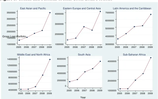
(17) poverty in a country. An increase of MFI loans may be accompanied by an increase in number of borrowers or an increase in the amount of loans each borrower receives. The latter is used in the second variant. Corresponding to these, the IV estimation uses log of GLPMF for the first case and log of [GLPMF/NOABMF] for the second case. In addition to the cross-sectional estimations, we generate panel data for 2003 and 2007 for all the variables16 and estimate linear panel models. This construction enables us to examine the robustness of our coefficients as the panel data estimation takes account of changes of variables over time and unobservable country or regional-level effects. Our aim is to further examine the hypothesis that higher gross loan portfolio leads to poverty reduction at macro level. One of the important limitations pointed out by micro-studies is that microfinance or microcredit does not necessarily reach the poorest of the poor (e.g. Morduch, 1999). To further investigate this from the macro perspective, we examine the effects of gross loan portfolio on poverty gap (which measures depth of poverty) and squared poverty gap (which measures severity of poverty).. V.. Results. Figures 1 to 3 below, describe the patterns and trends in size and outreach of the microfinance industry using real gross loan portfolio (after adjusting inflation), number of MFIs and active borrowers. Overall, the compound growth rate of the median gross loan portfolio increases for all regions over the period 2005 to 2009. However, there are variations (steep and gentle) in the year-by-year upward slopes, while in one instance 16. Due to data constraints on the international poverty data, we took averages for the period 2000 to 2003 and 2004 to 2007 for poverty.. 16.

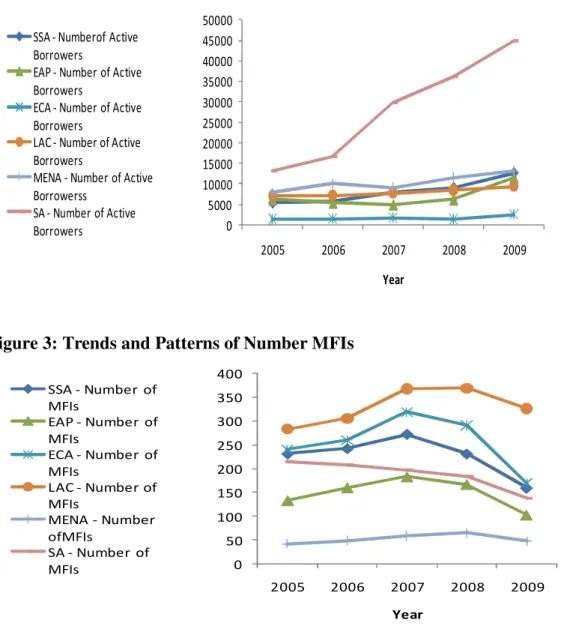
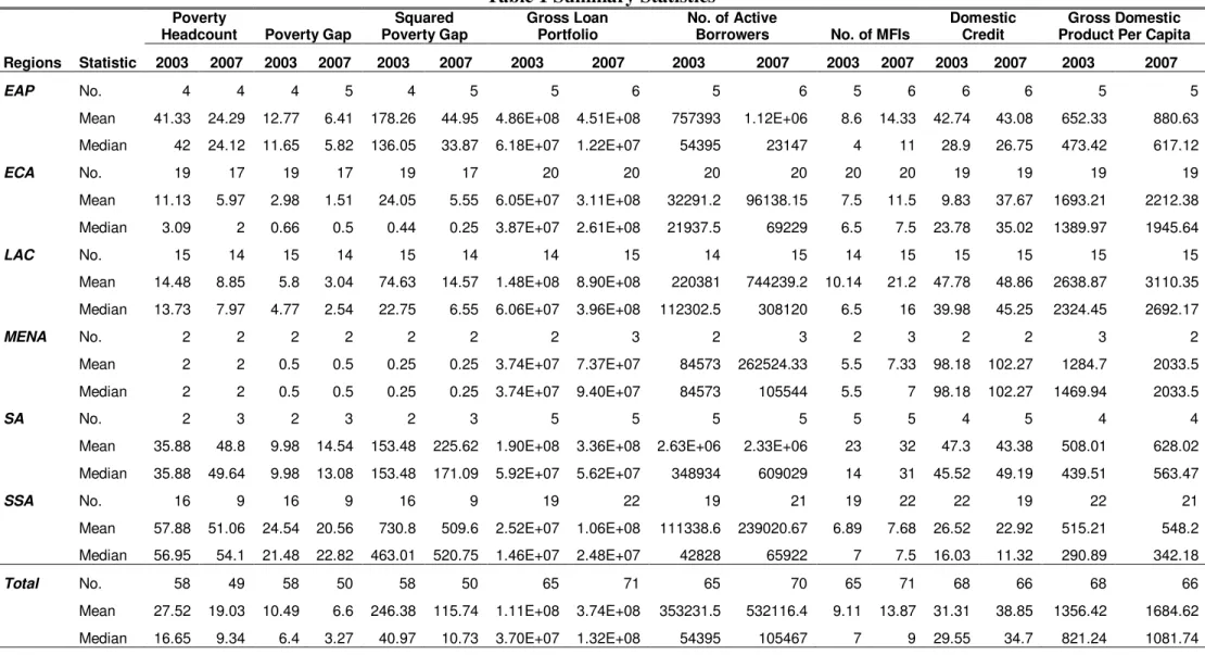
(18) (Eastern Europe and Central Asia), a downward trend is observed. In particular, the slope for 2007 to 2008 is either gently increasing or sloping downwards. An interpretation of the trend over this period will need to take cognizance of the potential adverse effect of the global financial crisis on the microfinance industry. Until 2007, the largest MFIs were located in Latin America and the Caribbean (LAC). However, in 2008, MFIs in Middle East and North Africa (MENA) experienced a sharp increase in their gross loan portfolio. Comparison of the patterns and trends of gross loan portfolio with the greater and sharp increase in number of active borrowers in South Asia (Figure 2) would trigger a number of questions, especially when using either of these indicators as a measure of microfinance operations in a country. Two reasons can be respectively surmised for the greater and sharp increase in South Asia’s number of active borrowers. Firstly, one can argue that by virtue of population size of countries in this region, it is by no means surprising that MFIs are able to reach out to more clients (scale of outreach). Secondly, differences in the mission of MFIs as a result of country (regional) level influences can account for the variation in the scale of outreach (number of clients). Thus, MFI’s with outreach focus (poverty-reducing) are likely to reach out to more clients. Numbers of MFIs in different regions and over time present another challenge in choosing an index to measure microfinance operations in a country. Figure 3 shows that LAC consistently (since 2005) has the highest number of MFIs in spite of its relatively smaller number of active borrowers, compared to South Asia (SA) and MENA. Table 1 provides a summary statistics of the variables used in the regression analyses. We report both mean and median of each variable for 2003 and 2007 for the respective. 17.

(19) regions. The rationale for reporting the median alongside the mean is to provide a further justification for the choice of the median as a descriptive statistic (and the need to use the logarithmic form of variables with high standard deviations (skewness) for the regression analyses). In view of the heterogeneity of the size of MFIs (gross loan portfolio), outreach (number of active borrowers), and a nation’s output per head (GDPPC), it is always prudent to observe the dispersion of the data. Table 1 indicates that the median in some instances is about either a hundredth (East Asia and the Pacific (EAP)) or a tenth (MENA) of the mean. This suggests that the raw data for the mean are likely to be affected by extreme values. Figure 1: Trends and Patterns of Real Gross Loan Portfolio East Asian and Pacific. Eastern Europe and Central Asia. 3500000. Latin America and the Cariibbean 7000000. 4000000. 3000000. 6000000 3000000. 2500000. 5000000 2000000 2000000. Gross Loan Portfolio. 4000000. 1500000 1000000. 1000000 2005. 2006. 2007. 2008. 2009. 3000000 2005. Middle East and North Africa. 2006. 2007. 2008. 2009. 2005. South Asia. 2006. 2007. 2008. 2009. Sub-Saharan Africa. 8000000. 14000000. 4000000 12000000. 6000000 3000000. 10000000. 4000000. 8000000 2000000. 2000000. 6000000 0 4000000. 2005 2005. 2006. 2007. 2008. 2006. 2007. 2009. 2008. 2009. 1000000 2005. Year. 18. 2006. 2007. 2008. 2009.

(20) Figure 2: Trends and Patterns of Number of Active Borrower SSA - Numberof Active Borrowers EAP - Number of Active Borrowers ECA - Number of Active Borrowers LAC - Number of Active Borrowers MENA - Number of Active Borrowerss SA - Number of Active Borrowers. 50000 45000 40000 35000 30000 25000 20000 15000 10000 5000 0 2005. 2006. 2007. 2008. 2009. Year. Figure 3: Trends and Patterns of Number MFIs 400 SSA - Number of MFIs EAP - Number of MFIs ECA - Number of MFIs LAC - Number of MFIs MENA - Number ofMFIs SA - Number of MFIs. 350 300 250 200 150 100 50 0 2005. 2006. 2007. 2008. 2009. Year. From the perspective of both numbers of active borrowers and MFIs, microfinance activities in SA countries are more intense than in the other regions. At the lower end, MFI activities in Sub-Saharan Africa (SSA) countries tend to show the lowest values for the number of active borrowers (as a proxy for MFI operations). As observed from the trends (Figures 1–3), variations in these indicators over time and across different regions suggest the need to develop a meaningful index that pulls together all three variables. In terms of the macro indicators, SSA, as expected, is the poorest region for both. 19.

(21) periods irrespective of the measure (incidence, depth and severity) in question. Over the period 2003 - 2007, both the poverty headcount and poverty gap showed a decline of about 7 and 4 percentage points, respectively.17 An exception is worth mentioning as our sample showed that poverty levels rose in South Asia over this period.18 Among the less ‘worse off’ regions,19 MENA recorded the lowest poverty headcount ratio while LAC showed the highest output per head (GDPPC) in both years. The poverty headcount ratio continued to be low (2%) in MENA, while it substantially decreased from 14.5% to 8.9% in LAC.. 17. Poverty data for the panel were constructed by taking averages for 2000-03 and 2004-07. The data are given in the Appendix 5. 18 It is noted that an overall increase in poverty in South Asia is due to the highly unbalanced nature of our panel data of poverty. As shown in Appendix 5, while Bangladesh has two observations, India, Nepal and Sri Lanka have only one either for 2003 or 2007. Despite the fall in poverty headcount for Bangladesh from 57.8% in 2003 to 49.6% in 2007, including countries with high poverty (e.g. Nepal- 55.1%) in 2007 accounts for the higher figure in 2007. 19 Most of the countries used in the study are either transitional or developing countries. This is because MFIs mostly evolve in countries with a high level of deprivation (mainly access to finance).. 20.

(22) Table 1 Summary Statistics Poverty Headcount Regions. Statistic. EAP. No.. 2007. SA. SSA. Total. 4. 4. 4. 5. 4. 5. 5. 6. 5. 6. 5. 6. 6. 6. 5. 5. 41.33. 24.29. 12.77. 6.41. 178.26. 44.95. 4.86E+08. 4.51E+08. 757393. 1.12E+06. 8.6. 14.33. 42.74. 43.08. 652.33. 880.63. Median. 42. 24.12. 11.65. 5.82. 136.05. 33.87. 6.18E+07. 1.22E+07. 54395. 23147. 4. 11. 28.9. 26.75. 473.42. 617.12. No.. 19. 17. 19. 17. 19. 17. 20. 20. 20. 20. 20. 20. 19. 19. 19. 19. 11.13. 5.97. 2.98. 1.51. 24.05. 5.55. 6.05E+07. 3.11E+08. 32291.2. 96138.15. 7.5. 11.5. 9.83. 37.67. 1693.21. 2212.38. 3.09. 2. 0.66. 0.5. 0.44. 0.25. 3.87E+07. 2.61E+08. 21937.5. 69229. 6.5. 7.5. 23.78. 35.02. 1389.97. 1945.64. 15. 14. 15. 14. 15. 14. 14. 15. 14. 15. 14. 15. 15. 15. 15. 15. Mean. 14.48. 8.85. 5.8. 3.04. 74.63. 14.57. 1.48E+08. 8.90E+08. 220381. 744239.2. 10.14. 21.2. 47.78. 48.86. 2638.87. 3110.35. Median. 13.73. 7.97. 4.77. 2.54. 22.75. 6.55. 6.06E+07. 3.96E+08. 112302.5. 308120. 6.5. 16. 39.98. 45.25. 2324.45. 2692.17. No.. 2. 2. 2. 2. 2. 2. 2. 3. 2. 3. 2. 3. 2. 2. 3. 2. Mean. 2. 2. 0.5. 0.5. 0.25. 0.25. 3.74E+07. 7.37E+07. 84573. 262524.33. 5.5. 7.33. 98.18. 102.27. 1284.7. 2033.5. Median. 2. 2. 0.5. 0.5. 0.25. 0.25. 3.74E+07. 9.40E+07. 84573. 105544. 5.5. 7. 98.18. 102.27. 1469.94. 2033.5. No.. 2. 3. 2. 3. 2. 3. 5. 5. 5. 5. 5. 5. 4. 5. 4. 4. Mean. 35.88. 48.8. 9.98. 14.54. 153.48. 225.62. 1.90E+08. 3.36E+08. 2.63E+06. 2.33E+06. 23. 32. 47.3. 43.38. 508.01. 628.02. Median. 35.88. 49.64. 9.98. 13.08. 153.48. 171.09. 5.92E+07. 5.62E+07. 348934. 609029. 14. 31. 45.52. 49.19. 439.51. 563.47. 16. 9. 16. 9. 16. 9. 19. 22. 19. 21. 19. 22. 22. 19. 22. 21. Mean. 57.88. 51.06. 24.54. 20.56. 730.8. 509.6. 2.52E+07. 1.06E+08. 111338.6. 239020.67. 6.89. 7.68. 26.52. 22.92. 515.21. 548.2. Median. 56.95. 54.1. 21.48. 22.82. 463.01. 520.75. 1.46E+07. 2.48E+07. 42828. 65922. 7. 7.5. 16.03. 11.32. 290.89. 342.18. 58. 49. 58. 50. 58. 50. 65. 71. 65. 70. 65. 71. 68. 66. 68. 66. Mean. 27.52. 19.03. 10.49. 6.6. 246.38. 115.74. 1.11E+08. 3.74E+08. 353231.5. 532116.4. 9.11. 13.87. 31.31. 38.85. 1356.42. 1684.62. Median. 16.65. 9.34. 6.4. 3.27. 40.97. 10.73. 3.70E+07. 1.32E+08. 54395. 105467. 7. 9. 29.55. 34.7. 821.24. 1081.74. 21. 2003. 2007. Gross Domestic Product Per Capita. 2003. No.. 2007. Domestic Credit. 2007. No.. 2003. No. of MFIs 2003. No.. 2007. No. of Active Borrowers. 2003. Median. MENA. 2003. Gross Loan Portfolio. 2007. Mean. LAC. Squared Poverty Gap. 2003. Mean. ECA. Poverty Gap. 2007. 2003. 2007.

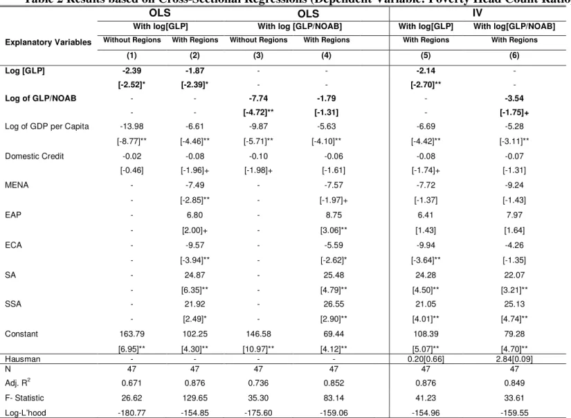
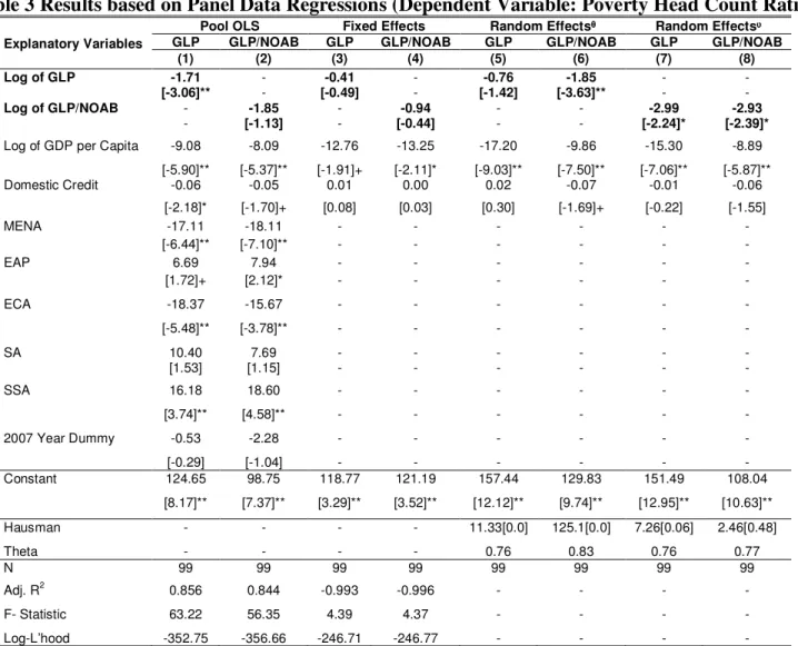
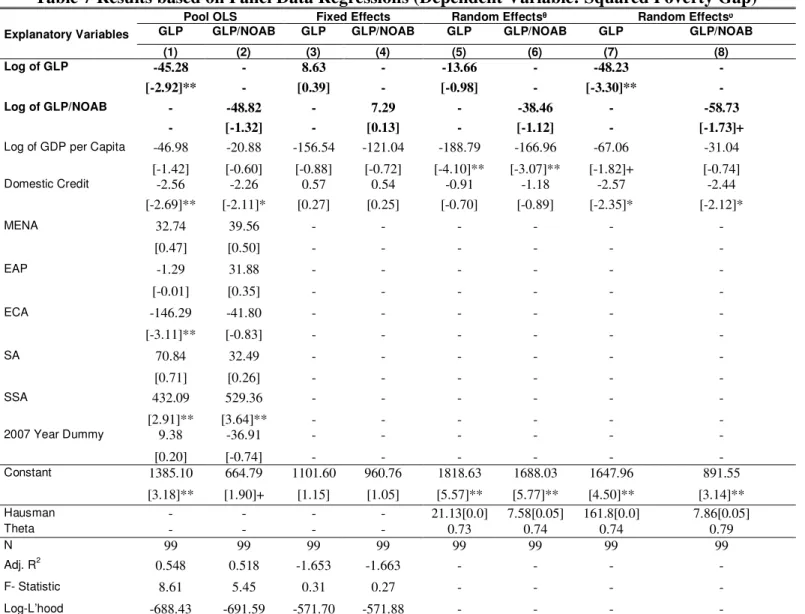
(23) The results of multivariate regressions are given in Tables 2 to 7 and simulation outcomes in Table 8. With a view to examining the hypothesis of a relationship between gross loan portfolio and poverty (incidence, depth and severity), fourteen different cases (i.e., six for cross-sectional regressions and eight for panel data regression) are examined for each poverty measure. Six different cases using cross section data for 2007 are given in Tables 2, 4 and 6 and eight cases are given in Tables 3, 5 and 7, using two-period (2003 and 2007) panel data. In Tables 2, 4 and 6, OLS is applied for columns (1) to (4) and IV for columns (5) and (6). The estimations in columns (1) to (4) are robust (corrected for heteroscedasticity), and examine cases either using GLP with and without regional dummies, or GLP/NOAB with and without regional dummies. The different specifications are motivated by policy concerns that underlie each of the cases. In a similar fashion, the IV (columns (5) and (6) of Tables 2, 4 and 6) and panel (Tables 3, 5 and 7) estimations examine the cases for GLP and GLP/NOAB. Three measures of the FGT class of poverty indices are used. Thus, Tables 2 and 3 contain all the estimations (OLS, IV, Fixed Effects (FE) and Random Effects (RE)) for the poverty headcount ratio; Tables 4 and 5 considers the case for the poverty gap (depth) and Tables 6 and 7 investigates the severity of poverty (squared gap).. 22.

(24) Table 2 Results based on Cross-Sectional Regressions (Dependent Variable: Poverty Head Count Ratio) OLS Explanatory Variables Log [GLP] Log of GLP/NOAB Log of GDP per Capita. Domestic Credit. MENA. EAP. ECA. SA. SSA. IV. OLS. With log[GLP]. With log [GLP/NOAB]. With log[GLP]. With log[GLP/NOAB]. Without Regions. With Regions. Without Regions. With Regions. With Regions. With Regions. (1). (2). (3). (4). (5). (6) -. -2.39. -1.87. -. -. -2.14. [-2.52]*. [-2.39]*. -. -. [-2.70]**. -. -. -. -7.74. -1.79. -. -3.54. -. -. [-4.72]**. [-1.31]. -. [-1.75]+. -13.98. -6.61. -9.87. -5.63. -6.69. -5.28. [-8.77]**. [-4.46]**. [-5.71]**. [-4.10]**. [-4.42]**. [-3.11]**. -0.02. -0.08. -0.10. -0.06. -0.08. -0.07. [-0.46]. [-1.96]+. [-1.98]+. [-1.61]. [-1.74]+. [-1.31]. -. -7.49. -. -7.57. -7.72. -9.24. -. [-2.85]**. -. [-1.97]+. [-1.37]. [-1.43]. -. 6.80. -. 8.75. 6.41. 7.97. -. [2.00]+. -. [3.06]**. [1.43]. [1.64]. -. -9.57. -. -5.59. -9.94. -4.26. -. [-3.94]**. -. [-2.62]*. [-3.64]**. [-1.35]. -. 24.87. -. 25.48. 24.28. 22.07. -. [6.35]**. -. [4.79]**. [4.50]**. [3.21]**. -. 21.92. -. 26.55. 21.05. 25.13. -. [2.49]*. -. [2.90]**. [4.01]**. [4.74]**. Constant. 163.79. 102.25. 146.58. 69.44. 108.39. 79.28. Hausman N. [6.95]** 47. [4.30]** 47. [10.97]** 47. [4.12]** 47. [5.07]** 0.20[0.66] 47. [4.70]** 2.84[0.09] 47. 0.671. 0.876. 0.736. 0.852. 0.876. 0.849. 26.62. 129.65. 35.30. 83.14. 41.23. 33.61. Adj. R. 2. F- Statistic Log-L’hood. -180.77 -154.85 -175.60 -159.06 -154.96 -159.55 ** Significant at one percent; * significant at five percent; † significant at 10 percent; t-values are in parenthesis. 23.

(25) Table 3 Results based on Panel Data Regressions (Dependent Variable: Poverty Head Count Ratio) Explanatory Variables Log of GLP Log of GLP/NOAB Log of GDP per Capita. Pool OLS GLP GLP/NOAB (1) (2) -1.71 [-3.06]** -1.85 [-1.13]. Fixed Effects GLP GLP/NOAB (3) (4) -0.41 [-0.49] -0.94 [-0.44]. Random Effectsᶿ GLP GLP/NOAB (5) (6) -0.76 -1.85 [-1.42] [-3.63]** -. Random Effectsᶹ GLP GLP/NOAB (7) (8) -2.99 -2.93 [-2.24]* [-2.39]*. -9.08. -8.09. -12.76. -13.25. -17.20. -9.86. -15.30. -8.89. [-5.90]** -0.06. [-5.37]** -0.05. [-1.91]+ 0.01. [-2.11]* 0.00. [-9.03]** 0.02. [-7.50]** -0.07. [-7.06]** -0.01. [-5.87]** -0.06. [-2.18]* -17.11 [-6.44]** 6.69 [1.72]+. [-1.70]+ -18.11 [-7.10]** 7.94 [2.12]*. [0.08] -. [0.03] -. [0.30] -. [-1.69]+ -. [-0.22] -. [-1.55] -. -18.37. -15.67. -. -. -. -. -. -. [-5.48]**. [-3.78]**. -. -. -. -. -. -. SA. 10.40 [1.53]. 7.69 [1.15]. -. -. -. -. -. -. SSA. 16.18. 18.60. -. -. -. -. -. -. [3.74]**. [4.58]**. -. -. -. -. -. -. Domestic Credit MENA EAP ECA. 2007 Year Dummy Constant. Hausman Theta N Adj. R. 2. F- Statistic. -0.53. -2.28. -. -. -. -. -. -. [-0.29] 124.65. [-1.04] 98.75. 118.77. 121.19. 157.44. 129.83. 151.49. 108.04. [8.17]**. [7.37]**. [3.29]**. [3.52]**. [12.12]**. [9.74]**. [12.95]**. [10.63]**. -. -. -. -. 11.33[0.0]. 125.1[0.0]. 7.26[0.06]. 2.46[0.48]. 99. 99. 99. 99. 0.76 99. 0.83 99. 0.76 99. 0.77 99. 0.856. 0.844. -0.993. -0.996. -. -. -. -. 63.22. 56.35. 4.39. 4.37. -. -. -. -. Log-L’hood -352.75 -356.66 -246.71 -246.77 ** Significant at one percent; * significant at five percent; † significant at 10 percent; t-values are in parenthesis ; ᶿ nation effect; and ᶹ regional effect. 24.

(26) In column (1) of Table 2, all three specifications using the cross section data shows that GLP is negatively and significantly associated with a poverty headcount ratio, which is consistent with our hypothesis that GLP reduces poverty. Because MFI loan is defined in log, we observe that a 1% increase in MFI loan reduces poverty by 0.0214% in the case of the IV estimation (in column (5) of Table 2).20 The coefficient estimate of log of gross loan portfolio of MFI is negative and significant at 1% level. As expected, GDP per capita is negative and shows a 1% statistical significance irrespective of the specification or the estimation method chosen. Also, consistent with the finance-poverty literature, we also find that the coefficient estimate of share of domestic credit to GDP is negative and significant in some cases (columns (2), (3) and (5) of Table 2). Columns (2) and (4) explore the potential effect of regional dummies on incidence of poverty using log of gross loan portfolio and log of loan per borrower respectively. Log of gross loan portfolio of MFI is negative and significant at the 5% level. The effect of log of loan per borrower is significant in the IV estimation, but not in the OLS. Inclusion of regional dummies in the poverty headcount equation reveals that ECA, with LAC as the reference case, has a significant negative coefficient (at the 5% level in three out of the four cases). Also, SA and SSA dummies are positive with a higher level of statistical significance in all four cases. This implies that SA and SSA have higher poverty headcount levels relative to LAC. These regression results are consistent with the summary statistics of Table 1, where both poverty levels and GDPPC shows that SA and SSA trail LAC. Columns (5) and (7) present the IV estimation with the aim of resolving the potential 20. This is based on the formulae to interpret the coefficient of semi-log specification (level-log): ∆Y= (β/100) % ∆X (Wooldridge, 2009, p.46). Note that poverty headcount ratio is defined in percentages.. 25.

(27) endogeneity of microfinance variables in the poverty headcount equation, that is, gross loan portfolio and number of active borrowers. As discussed earlier, the endogeneity may be due to either bi-causality or measurement errors depending on the variable in question. For instance, in terms of a bi-causal relationship between gross loan portfolio and poverty headcount, we allude to the fact that investors who are inclined to poverty reduction might direct their financial resources to countries and regions where poverty is high. Appendices 2 and 3 show the correlation matrix and the first stage IV estimation which offer a justification for the validity of our instruments. Instruments used in the two cases of columns (5) and (6) are weighted five-year lag of gross loan portfolio for the equation using GLP and weighted five-year lag of gross loan portfolio/ weighted five-year lag of number of active borrowers for the case of loan per borrower. In the case of loan per borrower, the Hausman test favours IV estimates over OLS, and this validates our use of the IV model. All the signs of the explanatory remain unchanged. We do not report the Sargan test as the instruments are exactly identified.. 26.

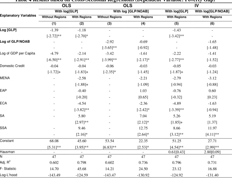
(28) Table 4 Results based on Cross-Sectional Regressions (Dependent Variable: Poverty Gap) OLS. OLS. With log[GLP] Explanatory Variables. Log [GLP] Log of GLP/NOAB Log of GDP per Capita. Domestic Credit. MENA. EAP. ECA. IV. With log [GLP/NOAB]. With log[GLP]. With log[GLP/NOAB]. Without Regions. With Regions. Without Regions. With Regions. With Regions. With Regions. (1). (2). (3). (4). (5). (6). -1.39 [-2.72]** -4.79. -1.18 [-2.70]* -2.14. -2.92 [-3.65]** -3.42. -0.69 [-0.92] -1.61. -1.43 [-3.42]** -2.22. -1.65 [-1.48] -1.41. [-6.50]**. [-2.91]**. [-3.99]**. [-2.17]*. [-2.77]**. [-1.52]. -0.04 [-1.72]+. -0.04 [-1.83]+. -0.06 [-2.35]*. -0.03 [-1.45]. -0.05 [-1.87]+. -0.03 [-1.24]. -. -2.58. -. -2.21. -2.79. -3.12. -. [-1.88]+. -. [-1.09]. [-0.94]. [-0.88]. -. -0.40. -. 1.03. -0.76. 0.60. -. [-0.20]. -. [0.65]. [-0.32]. [0.23]. -. -4.54. -. -2.36. -4.89. -1.63. -. [-3.82]**. -. [-2.42]*. [-3.39]**. [-0.94]. SA. -. 5.80. -. 7.04. 5.26. 5.19. SSA. -. [2.97]** 9.46. -. [2.12]* 12.75. [1.85]+ 8.66. [1.37] 11.97. -. [2.16]*. -. [2.64]*. [3.12]**. [4.11]**. Constant. 68.08. 45.60. 53.54. 22.35. 51.25. 27.71. Hausman N. [5.31]** 47 0.602. [3.95]** 47 0.798. [6.83]** 47 0.602. [2.53]* 47 0.736. [4.54]** 0.61[0.43] 47 0.796. [2.99]** 2.80[0.09] 47 0.731. 14.70. 45.68. 14.21. 24.50. 23.12. 16.88. -143.49. -124.59. -143.47. -130.92. -124.92. -131.40. Adj. R. 2. F- Statistic Log-L’hood. ** Significant at one percent; * significant at five percent; † significant at 10 percent; t-values are in parenthesis. 27.

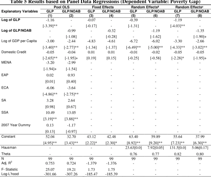
(29) Table 5 Results based on Panel Data Regressions (Dependent Variable: Poverty Gap) Explanatory Variables Log of GLP Log of GLP/NOAB Log of GDP per Capita Domestic Credit MENA. EAP. ECA. SA. SSA. GLP (1). Pool OLS GLP/NOAB (2). Fixed Effects GLP GLP/NOAB (3) (4). Random Effectsᶿ GLP GLP/NOAB (5) (6). Random Effectsᶹ GLP GLP/NOAB (7) (8). -1.16 [-3.39]** -3.00. -0.99 [-1.08] -2.44. -0.07 [-0.17] -4.83. -0.32 [-0.28] -4.61. -0.39 [-1.31] -6.72. -1.19 [-1.62] -6.02. -1.19 [-4.03]** -3.30. -1.35 [-1.90]+ -2.66. [-3.40]** -0.05 [-2.65]** -3.20. [-2.77]** -0.04 [-1.95]+ -2.99. [-1.34] 0.01 [0.19] -. [-1.37] 0.01 [0.15] -. [-6.49]** -0.01 [-0.25] -. [-5.00]** -0.02 [-0.58] -. [-4.33]** -0.05 [-2.28]* -. [-3.02]** -0.05 [-1.95]+ -. [-1.94]+. [-1.54]. -. -. -. -. -. -. 0.02. 0.93. -. -. -. -. -. -. [0.01]. [0.40]. -. -. -. -. -. -. -6.06. -3.64. -. -. -. -. -. -. [-4.86]**. [-2.75]**. -. -. -. -. -. -. 3.28. 2.64. -. -. -. -. -. -. [0.98] 10.49. [0.67] 13.05. -. -. -. -. -. -. [3.19]**. [3.88]**. -. -. -. -. -. -. 0.13. -1.17. -. -. -. -. -. -. Constant. [0.13] 52.04. [-0.97] 32.70. 43.12. 42.48. 63.40. 59.89. 55.64. 37.99. Hausman. [4.95]** -. [3.43]** -. [2.22]* -. [2.30]* -. [8.92]** 23.63[0.0]. [9.20]** 7.92[0.05]. [7.23]** 131.5[0.0]. [6.30]** 5.06[0.17]. 99 0.753. 99 0.724. 99 -1.379. 99 -1.376. 0.76 99 -. 0.77 99 -. 0.82 99 -. 0.80 99 -. 2007 Year Dummy. Theta N 2 Adj. R. F- Statistic 25.07 19.21 1.73 1.75 Log-L’hood -301.66 -307.26 -185.47 -185.39 ** Significant at one percent; * significant at five percent; † significant at 10 percent; t-values are in parenthesis ; ᶿ nation effect; and ᶹ regional effect. 28.

(30) Tables 3, 5 and 7 show the results based on panel estimations for the poverty headcount ratio, depth and severity, respectively. In Table 3, the poverty headcount ratio is estimated by the same set of explanatory variables. The number of observation is 99. It is noted that this estimation is based on highly unbalanced panel data and thus the results have to be interpreted with caution (see Appendix 4 for the list of countries and frequencies of observations). A similar pattern of results is observed, that is, gross loan portfolio of microfinance institutions is negatively associated with incidence of poverty, after controlling for the effects of other covariates and unobserved heterogeneity. In Tables 4 and 5, we have replicated both the cross-sectional and panel regressions by replacing the poverty headcount ratio with the poverty gap. To avoid cluttering the text, we summarise the key findings. All three cases show significant negative effects of log of gross loan portfolio of MFIs, implying the potential of microfinance in reducing the depth of poverty. The other explanatory variables show expected signs too. In columns (4) and (6), log of loan per borrower has negative but non-significant coefficients. The results of IV estimations in column (6) of Table 3 support our hypothesis that GLP reduces poverty gap but the evidence is weak. This hypothesis is further corroborated by random effects estimations in columns (7) and (8) of Table 5. In both cases (GLP and loan per borrower), there is a significant negative effect. Both the Hausman and theta statistics favour random effects over fixed effects.. 29.

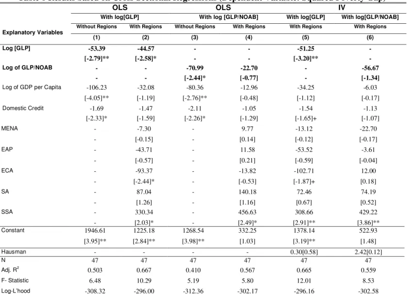
(31) Table 6 Results based on Cross-Sectional Regressions (Dependent Variable: Squared Poverty Gap) OLS. OLS. With log[GLP] Explanatory Variables Log [GLP] Log of GLP/NOAB Log of GDP per Capita. Domestic Credit. MENA. EAP. ECA. IV. With log [GLP/NOAB]. With log[GLP]. With log[GLP/NOAB]. Without Regions. With Regions. Without Regions. With Regions. With Regions. With Regions. (1). (2). (3). (4). (5). (6). -53.39 [-2.79]** -106.23. -44.57 [-2.58]* -32.08. -70.99 [-2.44]* -80.36. -22.70 [-0.77] -12.96. -51.25 [-3.20]** -34.25. -56.67 [-1.34] -6.03. [-4.05]**. [-1.19]. [-2.76]**. [-0.48]. [-1.12]. [-0.17]. -1.69 [-2.33]*. -1.47 [-1.59]. -2.11 [-2.26]*. -1.05 [-1.29]. -1.54 [-1.65]+. -1.13 [-1.07]. -. -7.30. -. 9.77. -13.12. -22.70. -. [-0.15]. -. [0.14]. [-0.12]. [-0.17]. -. -43.71. -. 11.58. -53.52. -3.61. -. [-0.57]. -. [0.21]. [-0.59]. [-0.04]. -. -93.37. -. -13.82. -102.71. 12.00. -. [-2.44]*. -. [-0.53]. [-1.87]+. [0.18]. SA. -. 87.04. -. 140.18. 72.46. 74.19. SSA. -. [1.26] 330.34. -. [1.16] 456.63. [0.67] 308.66. [0.52] 429.22. 1946.61. [2.03]* 1225.18. 1268.54. [2.49]* 332.25. [2.91]** 1378.14. [3.86]** 522.93. [3.95]**. [2.84]**. [3.98]**. [1.03]. [3.19]**. [1.48]. 47 0.503. 47 0.667. 47 0.410. 47 0.567. 0.30[0.58] 47 0.665. 2.42[0.12] 47 0.559. Constant. Hausman N Adj. R. 2. F- Statistic. 6.48. 10.29. 5.19. 5.80. 12.01. 8.53. Log-L’hood. -308.32. -296.00. -312.36. -302.17. -296.16. -302.58. ** Significant at one percent; * significant at five percent; † significant at 10 percent; t-values are in parenthesis. 30.

(32) Table 7 Results based on Panel Data Regressions (Dependent Variable: Squared Poverty Gap) Explanatory Variables Log of GLP Log of GLP/NOAB Log of GDP per Capita Domestic Credit. GLP. Pool OLS GLP/NOAB. Fixed Effects GLP GLP/NOAB. Random Effectsᶿ GLP GLP/NOAB. GLP. Random Effectsᶹ GLP/NOAB. (1). (2). (3). (4). (5). (6). (7). (8). -45.28 [-2.92]** -46.98. -48.82 [-1.32] -20.88. 8.63 [0.39] -156.54. 7.29 [0.13] -121.04. -13.66 [-0.98] -188.79. -38.46 [-1.12] -166.96. -48.23 [-3.30]** -67.06. -58.73 [-1.73]+ -31.04. [-1.42] -2.56 [-2.69]**. [-0.60] -2.26 [-2.11]*. [-0.88] 0.57 [0.27]. [-0.72] 0.54 [0.25]. [-4.10]** -0.91 [-0.70]. [-3.07]** -1.18 [-0.89]. [-1.82]+ -2.57 [-2.35]*. [-0.74] -2.44 [-2.12]*. 32.74. 39.56. -. -. -. -. -. -. [0.47]. [0.50]. -. -. -. -. -. -. EAP. -1.29. 31.88. -. -. -. -. -. -. [-0.01]. [0.35]. -. -. -. -. -. -. ECA. -146.29. -41.80. -. -. -. -. -. -. MENA. [-3.11]**. [-0.83]. -. -. -. -. -. -. SA. 70.84. 32.49. -. -. -. -. -. -. SSA. [0.71] 432.09. [0.26] 529.36. -. -. -. -. -. -. 2007 Year Dummy. [2.91]** 9.38. [3.64]** -36.91. -. -. -. -. -. -. Constant. [0.20] 1385.10. [-0.74] 664.79. 1101.60. 960.76. 1818.63. 1688.03. 1647.96. 891.55. [3.18]** 99 0.548. [1.90]+ 99 0.518. [1.15] 99 -1.653. [1.05] 99 -1.663. [5.57]** 21.13[0.0] 0.73 99 -. [5.77]** 7.58[0.05] 0.74 99 -. [4.50]** 161.8[0.0] 0.74 99 -. [3.14]** 7.86[0.05] 0.79 99 -. 8.61. 5.45. 0.31. 0.27. -. -. -. -. Hausman Theta N Adj. R. 2. F- Statistic. Log-L’hood -688.43 -691.59 -571.70 -571.88 ** Significant at one percent; * significant at five percent; † significant at 10 percent; t-values are in parenthesis ; ᶿ nation effect; and ᶹ regional effect. 31.

(33) Tables 6 and 7 report the cases where the dependent variable is squared poverty gap. An examination of the poverty gap and squared poverty gap results show consistent results in terms of sign and significance for both measures of GLP. Also, in the case of squared poverty gap, the Hausman test favours random effects. 21 Broadly, the results imply that GLP of MFIs benefits not just the poor but also the poorest. In sum, gross loan portfolio of MFIs is negatively associated with the incidence, depth and severity of poverty.. VI. Simulations That microfinance is impervious to the global recession following the financial crisis is debatable 22 . Some have argued that the slowdown of the global economy will impact negatively on microfinance as MFIs are now more closely linked to global financial markets than before. So there will be (i) a funding or liquidity impact, with greater refinancing risks for MFIs, and (ii) an economic impact, with financial performance affected by lower lending volumes, higher costs of funding, tighter net interest margins, and greater volatility in foreign exchange losses/gains. Magnoni and Powers (2009), for example, point out that, over 2009-10, the sector-wide microfinance will grow by some $28 billion less than anticipated before the crisis. Others are more optimistic. For example, Littlefield and Kneiding (2009) argue that the microfinance sector will survive the setbacks because of the strong foundations and vast untapped market of creditworthy. 21. In addition to the Hausman test, we calculate theta (measure of the extent of biasedness of random effects’ model) and we observe values close to one (greater than 0.75) for each of three estimations. This supports the fact that country/regional effects over time are important and cannot be ignored. Use of the theta, which is preferred due to the strong finite assumption underlying the Hausman Test, further supports our choice of fixed effects model. 22 For a comprehensive review, see Llanto and Badiolo (2010).. 32.

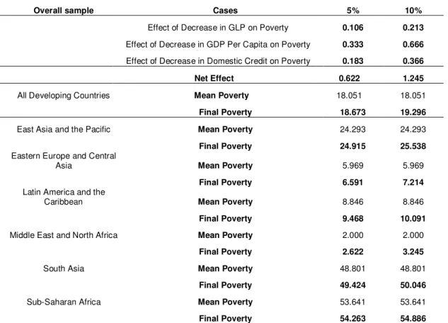
(34) clients. The effects on the poor through MFIs are, however, largely anecdotal. An attempt is made below to simulate the likely effects of the global recession.. Table 8 Effect of Decrease in GLP, GDP per capita and Domestic Credit on Poverty Overall sample. Cases. 5%. 10%. Effect of Decrease in GLP on Poverty. 0.106. 0.213. Effect of Decrease in GDP Per Capita on Poverty. 0.333. 0.666. Effect of Decrease in Domestic Credit on Poverty. 0.183. 0.366. Net Effect All Developing Countries. East Asia and the Pacific Eastern Europe and Central Asia Latin America and the Caribbean. Middle East and North Africa. South Asia. Sub-Saharan Africa. Mean Poverty. 0.622. 1.245. 18.051. 18.051. Final Poverty. 18.673. 19.296. Mean Poverty. 24.293. 24.293. Final Poverty. 24.915. 25.538. Mean Poverty. 5.969. 5.969. Final Poverty. 6.591. 7.214. Mean Poverty. 8.846. 8.846. Final Poverty. 9.468. 10.091. Mean Poverty. 2.000. 2.000. Final Poverty. 2.622. 3.245. Mean Poverty. 48.801. 48.801. Final Poverty. 49.424. 50.046. Mean Poverty. 53.641. 53.641. Final Poverty. 54.263. 54.886. In the context of the recent global recession, we examine the possible slowdown of poverty reduction23 as a result of contraction (i) in gross loan portfolio of MFIs, (ii) GDP per capita and (iii) domestic credit provided by banking institutions. Table 8 reports the simulation results on the basis of the IV estimation reported in column (5) of Table 2.. 23. Imai, Gaiha and Thapa (2010) report a slowdown in the rate of poverty reduction post 2000 relative to the 1990-decade.. 33.

(35) The calculations24 are premised on the assumption that the coefficient estimate of each variable is the same across different regions in the regression and thus the simulated effects of key variables on poverty are also the same. The second to fourth rows of Table 8 show that the effects GDP per capita and domestic credit are higher than those of GLP of MFIs. While this is plausible in view of the comparative contribution of MFI in an economy, the poverty increasing effect of 0.106% (or 0.233%) due to the 5% (or 10%) decline in GLP points to the need for sustainable flow of on-lending funds. Although the overall rise in poverty is low (about 3.45 per cent in the first scenario of a mild recession), it must be emphasized that this is additional to other cumulative effects of the global slowdown on poverty (investments, for example, continue to be sluggish).. VI.. Concluding Observations. Recent assessments of impact of microfinance –based largely on randomised trials-have led to questioning of claims of women’s empowerment and poverty reduction. The socalled ‘magic’ of microfinance has thus come under deep scrutiny and the findings of little or weak impacts are beginning to turn the tide against it. Not only are some of these studies are faulty in some respects, but the findings also cannot be accepted at face value. Besides, the faltering global economy has raised serious concerns about the immunity of the microfinance sector and its potential for poverty reduction. From this perspective, the preceding analysis centrred around the hypothesis that microfinance reduces poverty. We carried out tests using the cross-country data in 2007 24. The simulated effects of GLP and GDPPC are calculated with the semi-log (or ‘level-log’) specification (∆Y= (β/100) % ∆X), while the effect of domestic credit is based on the ‘levellevel’ specification (∆Y= β ∆X) (see Wooldridge, 2009, p.46 for details).. 34.

(36) and a panel for 2003 and 2007. Taking account of the endogeneity associated with loans from microfinance institutions (MFIs), there is robust confirmation that microfinance loans are significantly and negatively associated with poverty, i.e., a country with a higher MFIs’ gross loan portfolio tends to have lower poverty, after controlling for the effects of other factors influencing it. The negative relationship remains unchanged when the poverty headcount ratio is replaced by the poverty gap and squared poverty gap. These results suggest that microfinance not only reduces the incidence of poverty but also its depth and severity. The panel results further corroborate these findings. Other factors that contribute to poverty reduction include GDP per capita and share of credit in GDP (as a measure of financial development of an economy). Besides, there are significant regional effects. Our simulations point to worsening of poverty in a mild recession scenario with small reductions in gross loan portfolio, GDP per capita and share of credit in GDP. These simulations are helpful in adding precision to anecdotal evidence about how setbacks to MFIs hurt the poor. Indeed, sustained flows to MFIs may help avert to some extent accentuation of poverty as a consequence of the slow and faltering recovery of the global economy. In conclusion, assertions that microfinance is ‘oversold’ and lacks the ‘magic’ associated with it are widely off the mark, if not largely mistaken.. 35.

(37) References Ahlin C. and Lin J. (2006) “Luck or Skill? MFI Performance in Macroeconomic Context” Bureau for Research and Economic Analysis of Development, BREAD Working Paper No. 132, Centre for International Development, Harvard University, USA Ahlin C., Lin, J. and Maio, M. (2010) “Where Does Microfinance Flourish? Microfinance Institution Performance in Macroeconomic Context” Journal of Development Economics doi: 10.1016/j.jdeveco.2010.04.004. Armendariz de Aghion and J. Morduch (2005) The Economics of Microfinance, Cambridge: MIT Press. Banerjee, A., E. Duflo, R. Glennerster and C. Kinnan (2009) “The Miracle of Microfinance? Evidence from a Randomised Evaluation”, Cambridge, MA: Department of Economics, MIT, mimeo. Chen, S. and Ravallion, M. (2008) “The Developing World is Poorer than We Thought, but No Less Successful in the Fight against Poverty”, Policy Research Working Paper WPS 4703, Washington, DC: World Bank. Collins, D., J. Morduch, S. Rutherford and O. Ruthven (2009) Portfolios of the Poor: How the World’s Poor Live on $2 a Day? Princeton: NJ: Princeton University Press. Feigenberg, B., E. M. Field and R. Pande (2010) “Building Social Capital through Microfinance”, Cambridge: MA: RWP 10-019, Kennedy School, Harvard University.. 36.

(38) Foster, J., Greer, J., and Thorbecke, E. (1984) “A Class of. Decomposable Poverty Measures” Econometrica, 52, 761-766. Gaiha, R. and M. A. Nandhi (2009)” Microfinance, Self-help Groups and Empowerment in Maharashtra, in R. Jha (ed.) The Indian Economy Sixty Years After Independence, London: Palgrave Macmillan. Hulme D. and Mosley, P. (1996) Finance Against Poverty. Vol. 1. London: Routledge Imai S. K., Arun T. and Annim S. K. (2010) “Microfinance and Household Poverty Reduction: New Evidence from India” World Development 38 (12) (forthcoming ). Imai, S. K., Gaiha, R., and Thapa, G. (2010) “Is the Millennium Development Goal of Poverty Still Achievable? Role of Institutions, Finance and Openness” Oxford Development Studies, 38(3), 309-337. Imai S. K., and M. D. Azam, (2010) “Does Microfinance Reduce Poverty in Bangladesh? New Evidence from Household Panel Data”, Mimeo., University of Manchester. Kabeer, N. 1998, ‘‘‘Money Can’t Buy Me Love?”: Re-evaluating Gender, Credit and Empowerment in Rural Bangladesh’, Brighton: IDS Discussion Paper, 363. Kai H. and Hamori S. (2009) “Microfinance and Inequality” MPRA Paper No. 17572 http://mpra.ub.uni-muenchen.de/17572/. Karlan, D. and J. Zinman (2009) “Expanding Credit Access: Using Randomised Supply Decisions to Estimate the Impacts”, New Haven: Conn: Innovations for Poverty Action. Khandker, S. R. (2005) “Micro-finance and poverty: Evidence using panel data from Bangladesh,” The World Bank Economic Review, 19(2), 263–286.. 37.

(39) Llanto, G. M., and J. A. R. Badiola (2010) “The Impact of the Global Financial Crisis on Rural and Microfinance in Asia” Rome: APR, IFAD, mimeo. Magnoni, B., and J. Powers (2009) “Will the Bottom of the Pyramid Hit Bottom? The Effects of the Global Credit Crisis on the Microfinance Sector”, Micro Report No. 150, A Report Prepared for USAID. Microfinance Information Exchange (2010) “Regional Benchmarking Latin America and the Caribbean 2009 Benchmarks”, http://www.themix.org/sites/default/files/LAC%20Benchmarks%20Tables%202009% 20EN%20(Final).pdf Date Accessed: 24th August 2010 Morduch, J. (1999) “The role of subsidies in microfinance: evidence from the Grameen Bank,” Journal of Development Economics, 60, 229–248. Mosley, P. (2001) “Microfinance and poverty in Bolivia” Journal of Development Studies, 37(4), 101–132. Ravallion, M., Chen, S. and Sangraula, P. (2008) “Dollar a Day Revisited”, World Bank Policy Research Working Paper No. 4620, Washington, DC: World Bank. Rosenberg, R. (2010) “Does Microcredit Really Help Poor People?”, Washington DC: Focus Note No 59.CGAP. Srinivasan, N. (2009) Multiple Borrowing or Multiple lending – who is to blame for debt fatigue? http://microfinance.cgap.org/2009/08/28/multiple-borrowing-or-multiplelending-%E2%80%93-who-is-to-blame-for-debt-fatigue/ Date Accessed: 05th/04/10. Wooldridge, J. (2009) Introductory Econometric: A Modern Approach, 4th Edition, Mason, Ohio, South Western Educational Publishing.. 38.

(40) World Bank (2010) World Development Indicators 2010, Washington D.C.: Oxford University Press. Wright, G. A. N. and Rippey, P. (2003) “The Competitive Environment in Uganda: Implications for Microfinance Institutions and their Clients” http://www2.ids.ac.uk/impact/publications/joint_publications/The%20Competitive%2 0Environment%20in%20Uganda%20Synthesis%20-%20Wright%20et%20al.pdf Date Accessed: 5th/10/10.. 39.

(41) APPENDICES Appendix 1: List of Regions and Nations Regions. Nations. Regions. Nations. Cambodia. No . 53. East Asia and the Pacific East Asia and the Pacific East Asia and the Pacific East Asia and the Pacific. Middle East and North Africa. Sudan. Papua New Guinea East Timor Indonesia. 54 55 56. Middle East and North Africa Middle East and North Africa Middle East and North Africa. Palestine Yemen Egypt. East Asia and the Pacific. Laos. 57. Middle East and North Africa. Jordan. East Asia and the Pacific East Asia and the Pacific East Asia and the Pacific East Asia and the Pacific East Asia and the Pacific Eastern Europe and Central Asia Eastern Europe and Central Asia Eastern Europe and Central Asia Eastern Europe and Central Asia Eastern Europe and Central Asia Eastern Europe and Central Asia Eastern Europe and Central Asia Eastern Europe and Central Asia Eastern Europe and Central Asia Eastern Europe and Central Asia Eastern Europe and Central Asia Eastern Europe and Central Asia Eastern Europe and Central Asia Eastern Europe and Central Asia Eastern Europe and Central Asia Eastern Europe and Central Asia Eastern Europe and Central Asia Eastern Europe and Central Asia Eastern Europe and Central Asia Eastern Europe and Central Asia Eastern Europe and Central Asia Eastern Europe and Central Asia Eastern Europe and Central Asia Latin America and the Caribbean Latin America and the Caribbean. China, People's Republic of Samoa Vietnam Philippines Thailand Uzbekistan Hungary Georgia Tajikistan Armenia Montenegro Kazakhstan Kosovo Russia Mongolia Kyrgyzstan Macedonia Bulgaria Serbia Romania Turkey Moldova Ukraine Croatia Albania Bosnia and Herzegovina Poland Azerbaijan Peru Brazil. 58 59 60 61 62 63 64 65 66 67 68 69 70 71 72 73 74 75 76 77 78 79 80 81 82 83 84 85 86 87. Middle East and North Africa Middle East and North Africa Middle East and North Africa Middle East and North Africa Middle East and North Africa South Asia South Asia South Asia South Asia South Asia South Asia Sub-Saharan Africa Sub-Saharan Africa Sub-Saharan Africa Sub-Saharan Africa Sub-Saharan Africa Sub-Saharan Africa Sub-Saharan Africa Sub-Saharan Africa Sub-Saharan Africa Sub-Saharan Africa Sub-Saharan Africa Sub-Saharan Africa Sub-Saharan Africa Sub-Saharan Africa Sub-Saharan Africa Sub-Saharan Africa Sub-Saharan Africa Sub-Saharan Africa Sub-Saharan Africa. Syria Iraq Tunisia Morocco Lebanon Bangladesh India Nepal Afghanistan Pakistan Sri Lanka Tanzania Mozambique Benin Kenya Angola Togo Uganda Sierra Leone Gambia, The Senegal South Africa Guinea Cameroon Mali Malawi Cote d'Ivoire (Ivory Coast) Burkina Faso Swaziland Niger. Latin America and the Caribbean. Bolivia. 88. Sub-Saharan Africa. Guinea-Bissau. No. 1 2 3 4 5 6 7 8 9 10 11 12 13 14 15 16 17 18 19 20 21 22 23 24 25 26 27 28 29 30 31 32 33 34 35 36. 40.

(42) 37 38 39 40. Latin America and the Caribbean. Mexico. 89. Sub-Saharan Africa. Congo, Republic of the. Latin America and the Caribbean. Costa Rica. 90. Sub-Saharan Africa. Ethiopia. Latin America and the Caribbean. Guatemala. 91. Sub-Saharan Africa. Burundi. Latin America and the Caribbean. Colombia. 92. Sub-Saharan Africa. Nigeria. Latin America and the Caribbean. Trinidad and Tobago. 93. Sub-Saharan Africa. Latin America and the Caribbean. Venezuela. 94. Sub-Saharan Africa. Congo, Democratic Republic of the Chad. Latin America and the Caribbean. Haiti. 95. Sub-Saharan Africa. Central African Republic. Latin America and the Caribbean. Ecuador. 96. Sub-Saharan Africa. Rwanda. Latin America and the Caribbean Latin America and the Caribbean. Nicaragua Panama. 97 98. Sub-Saharan Africa Sub-Saharan Africa. Ghana Madagascar. Latin America and the Caribbean Latin America and the Caribbean Latin America and the Caribbean. Argentina Chile El Salvador. 99. Sub-Saharan Africa. Zambia. Latin America and the Caribbean. Paraguay. Latin America and the Caribbean. Honduras. Latin America and the Caribbean. Dominican Republic. 41 42 43 44 45 46 47 48 49 50 51 52. Appendix 3: Correlation Matrix Variables Poverty Headcount. Poverty Headcount. Poverty gap. Squared Poverty Gap. Log of GLP. Log of NOAB. 0.96. 1. Squared Poverty Gap. 0.84. 0.94. 1. -0.34. -0.38. -0.37. 1. Log of NOAB. Log of [W.GLP/W.NOAB]. Log of GDP per Capita. Domestic Credit. Log. W. GLP. Log of W. NOAB. 1. Poverty gap. Log of GLP. Log of GLP/NOAB. 0.04. -0.04. -0.11. 0.8. 1. Log of GLP/NOAB. -0.63. -0.55. -0.43. 0.44. -0.19. 1. Log of W.GLP/W.NOAB. -0.73. -0.65. -0.53. 0.47. 0.02. 0.83. 1. Log of GDP per Capita. -0.79. -0.69. -0.53. 0.28. -0.04. 0.52. 0.61. 1. Domestic Credit. -0.31. -0.32. -0.31. 0.09. 0.11. -0.01. 0.06. 0.46. 1. Log. W. GLP. -0.17. -0.28. -0.36. 0.85. 0.75. 0.28. 0.46. 0.3. 0.16. 1. 0.28. 0.13. -0.02. 0.63. -0.15. -0.06. 0.13. 0.81. Log of W. NOAB. 0.82 -0.24 W. – Weighted five-year lag average. 41. 1.

(43) Appendix 3: First Stage IV Estimation GLP 0.78 [6.60]**. Log of Weighted lag of Average GLP Log of Weighted lag of Average GLP/ Weighted lag of Average NoAB. GLP/NOAB. 0.83 [12.10]**. Log of GDP per Capita. -0.14 [-0.50] 0.00 [0.48] -0.78 [-0.73] -1.55 [-1.87]+ -0.19 [-0.37] -2.01 [-2.06]* -0.79 [-0.83] 5.82 [1.73]+ 47 0.548 7.97 -72.10. Domestic Credit MENA EAP ECA SA SSA Constant N Adjusted R-Squared F-Statistic Log-Likelihood. 0.00 [1.19] -0.68 [-2.70]* 0.12 [0.62] 0.13 [1.10] -0.45 [-1.79]+ 0.08 [0.40] 1.34 [2.71]** 47 0.923 79.59 -6.27. †. ** Significant at one percent; * significant at five percent; significant at 10 percent; t-values are in parenthesis. Appendix 4: List of Nations for Panel Data - Table 5 No.. Nations. Freq.. No.. Nations. 1. Albania. 2. 32. Kazakhstan. 2. 2. Armenia. 2. 33. Kenya. 1. 3. Azerbaijan. 2. 34. Kyrgyz Republic. 2. 4. Bangladesh. 2. 35. Macedonia, FYR. 2. 5. Benin. 1. 36. Madagascar. 2. 6. Bosnia and Herzegovina. 2. 37. Malawi. 1. 7. Brazil. 2. 38. Mexico. 2. 8. Bulgaria. 1. 39. Moldova. 2. 9. Burkina Faso. 1. 40. Mongolia. 2. 10. Cambodia. 1. 41. Mozambique. 1. 11. Cameroon. 1. 42. Nepal. 1. 12. Chile. 2. 43. Nicaragua. 2. 13. China. 2. 44. Panama. 1. 14. Colombia. 2. 45. Paraguay. 2. 15. Congo, Dem. Rep. of. 1. 46. Peru. 2. 16. Costa Rica. 2. 47. Poland. 2. 17. Croatia. 2. 48. Romania. 2. 18. Dominican Republic. 2. 49. Russia. 2. 19. East Timor. 1. 50. Rwanda. 1. 20. Ecuador. 2. 51. Sierra Leone. 1. 42. Freq..

(44) 21. Egypt, Arab Rep.. 2. 52. South Africa. 1. 22. El Salvador. 2. 53. Sri Lanka. 1. 23. Ethiopia. 2. 54. Swaziland. 1. 24. Georgia. 2. 55. Tajikistan. 2. 25. Guatemala. 2. 56. Tanzania. 1. 26. Guinea. 1. 57. Turkey. 2. 27. Haiti. 1. 58. Uganda. 2. 28. Honduras. 2. 59. Ukraine. 2. 29. India. 1. 60. Vietnam. 2. 30. Indonesia. 1. 61. Zambia. 2. 31. Jordan. 2. Appendix 5: International Poverty Data - Unbalanced Panel No.. Year. Nations. Poverty HC. No.. Year. Nations. Poverty HC. 1. 2003. Albania. 2.00. 54. 2007. Kenya. 19.72. 2. 2007. Albania. 2.00. 55. 2003. Kyrgyz Republic. 34.03. 3. 2003. Armenia. 12.20. 56. 2007. Kyrgyz Republic. 12.62. 4. 2007. Armenia. 3.65. 57. 2003. Macedonia, FYR. 2.31. 5. 2003. Azerbaijan. 6.32. 58. 2007. Macedonia, FYR. 2.00. 6. 2007. Azerbaijan. 2.00. 59. 2003. Madagascar. 76.34. 7. 2003. Bangladesh. 57.82. 60. 2007. Madagascar. 67.83. 8. 2007. Bangladesh. 49.64. 61. 2007. Malawi. 73.86. 9. 2003. Benin. 47.33. 62. 2003. Mexico. 4.28. 10. 2003. Bosnia and Herzegovina. 2.00. 63. 2007. Mexico. 2.40. 11. 2007. Bosnia and Herzegovina. 2.00. 64. 2003. Moldova. 25.05. 12. 2003. Brazil. 10.40. 65. 2007. Moldova. 5.26. 13. 2007. Brazil. 8.00. 66. 2003. Mongolia. 15.47. 14. 2003. Bulgaria. 2.32. 67. 2007. Mongolia. 22.38. 15. 2003. Burkina Faso. 56.54. 68. 2003. Mozambique. 74.69. 16. 2007. Cambodia. 33.02. 69. 2007. Nepal. 55.12. 17. 2003. Cameroon. 32.81. 70. 2003. Nicaragua. 19.42. 18. 2003. Chile. 2.00. 71. 2007. Nicaragua. 15.81. 19. 2007. Chile. 2.00. 72. 2007. Panama. 9.34. 20. 2003. China. 28.36. 73. 2003. Paraguay. 17.23. 21. 2007. China. 15.92. 74. 2007. Paraguay. 7.88. 22. 2003. Colombia. 16.07. 75. 2003. Peru. 13.84. 23. 2007. Colombia. 16.01. 76. 2007. Peru. 7.94. 24. 2007. Congo, Dem. Rep. of. 59.22. 77. 2003. Poland. 2.00. 25. 2003. Costa Rica. 4.52. 78. 2007. Poland. 2.00. 26. 2007. Costa Rica. 2.19. 79. 2003. Romania. 3.09. 27. 2003. Croatia. 2.00. 80. 2007. Romania. 2.00. 28. 2007. Croatia. 2.00. 81. 2003. Russia. 2.00. 43.

(45) 29. 2003. Dominican Republic. 5.27. 82. 2007. Russia. 2.00. 30. 2007. 31. 2003. Dominican Republic. 4.46. 83. 2003. Rwanda. 76.56. East Timor. 52.94. 84. 2003. Sierra Leone. 53.37. 32. 2003. Ecuador. 10.49. 85. 2003. South Africa. 26.20. 33. 2007. Ecuador. 7.24. 86. 2003. Sri Lanka. 13.95. 34. 2003. Egypt, Arab Rep.. 2.00. 87. 2003. Swaziland. 62.85. 35. 2007. Egypt, Arab Rep.. 2.00. 88. 2003. Tajikistan. 36.25. 36. 2003. El Salvador. 13.73. 89. 2007. Tajikistan. 21.49. 37. 2007. El Salvador. 8.70. 90. 2003. Tanzania. 88.52. 38. 2003. Ethiopia. 55.58. 91. 2003. Turkey. 2.00. 39. 2007. Ethiopia. 39.04. 92. 2007. Turkey. 2.65. 40. 2003. Georgia. 12.80. 93. 2003. Uganda. 57.37. 41. 2007. Georgia. 13.44. 94. 2007. Uganda. 51.53. 42. 2003. Guatemala. 14.99. 95. 2003. Ukraine. 2.00. 43. 2007. Guatemala. 11.70. 96. 2007. Ukraine. 2.00. 44. 2003. Guinea. 70.13. 97. 2003. Vietnam. 40.05. 45. 54.9. Haiti. 54.90. 98. 2007. Vietnam. 22.82. 46. 2003. Honduras. 18.10. 99. 2003. Zambia. 64.60. 47. 2007. Honduras. 20.19. 100. 2007. Zambia. 64.29. 48. 2003. India. 41.64. 49. 2007. Indonesia. 25.42. 50. 2003. Jordan. 2.00. 51. 2007. Jordan. 2.00. 52. 2003. Kazakhstan. 3.42. 53. 2007. Kazakhstan. 2.00. Source: Authors’ Compilation Based on 2010 World Development Indicators. 44.

(46)

No results found