SFB 649 Discussion Paper 2011-072
Financial Network Systemic
Risk Contributions
Nikolaus Hautsch*
Julia Schaumburg*
Melanie Schienle*
* Humboldt-Universität zu Berlin, Germany
This research was supported by the Deutsche
Forschungsgemeinschaft through the SFB 649 "Economic Risk". http://sfb649.wiwi.hu-berlin.de ISSN 1860-5664 SFB 649, Humboldt-Universität zu Berlin
S
FB
6
4
9
E
C
O
N
O
M
I
C
R
I
S
K
B
E
R
L
I
N
Financial Network Systemic Risk Contributions
∗
Nikolaus Hautsch
Julia Schaumburg
Melanie Schienle
October 21, 2011
ABSTRACT
We propose thesystemic risk betaas a measure for financial companies’ contribu-tion to systemic risk given network interdependence between firms’ tail risk expo-sures. Conditional on statistically pre-identified network spillover effects and market and balance sheet information, we define the systemic risk beta as the time-varying marginal effect of a firm’s Value-at-risk (VaR) on the system’s VaR. Suitable statis-tical inference reveals a multitude of relevant risk spillover channels and determines companies’ systemic importance in the U.S. financial system. Our approach can be used to monitor companies’ systemic importance allowing for a transparent macro-prudential regulation.
Keywords: Systemic risk contribution, systemic risk network, Value at Risk, net-work topology, two-step quantile regression, time-varying parameters
JEL classification:G01, G18, G32, G38, C21, C51, C63
The financial crisis 2007-2009 has shown that cross-sectional dependencies between as-sets and credit exposures can cause even small risks of individual banks to cascade and
∗ This paper replaces former working paper versions with title “Quantifying Time-Varying Marginal Systemic Risk Contributions”. Nikolaus Hautsch, Center for Applied Statistics and Economics (CASE), Humboldt-Universität zu Berlin and Center for Financial Studies, Frankfurt, email: [email protected]. Julia Schaumburg, Humboldt-Universität zu Berlin, email: [email protected]. Melanie Schienle, CASE and Humboldt-Universität zu Berlin, email: [email protected]. We thank Tobias Adrian, Markus Brunnermeier, Robert En-gle, Tony Hall, Simone Manganelli, Robin Lumsdaine and Christian Brownlees as well as participants of the annual meeting of the Society for Financial Econometrics (SoFiE) in Chicago, the 2nd Humboldt-Copenhagen Conference in Humboldt-Copenhagen and the 2011 annual European meeting of the Econometric Society in Oslo. Research supported by the Deutsche Forschungsgemeinschaft via the Collaborative Research Cen-ter 649 ”Economic Risk” is gratefully acknowledged.
build up to a substantial threat for the stability of an entire financial system.1 Under certain
economic conditions, company-specific risk cannot be appropriately assessed in isolation without accounting for potential risk spillover effects from other firms. In fact, it is not just its size and idiosyncratic risk but also its interconnectedness with other firms which deter-mines a company’s systemic relevance i.e., its potential to significantly increase the risk of failure of the entire system – which we denote as systemic risk.2 While there is a broad consensus that any prudential regulatory policy should account for the consequences of network interdependencies in the financial system, in practice, however, any attempt of a transparent implementation must fail, as long as suitable empirical measures for firms’ individual risk, risk spillovers and systemic relevance are not available. In particular, it is unclear how to quantify individual risk exposures and systemic risk contributions in an appropriate but still parsimonious and empirically tractable way for a prevailing underly-ing network structure. And there is an apparent need for respective empirically feasible and forward-looking measures which only rely on available data of publicly disclosed balance sheet and market information but still account for the complexity of the financial system.
A general empirical assessment of systemic relevance cannot build on the vast theo-retical literature of financial network models and financial contagion, since these results typically require detailed information on intra-bank asset and liability exposures (see, e.g., Allen and Gale, 2000, Freixas, Parigi, and Rochet, 2000, and Leitner, 2005). Such data is generally not publicly disclosed and even regulators can only collect partial informa-tion on some sources of inter-bank linkages. Available empirical studies linked to this literature can therefore only partially contribute to a full picture of companies’ systemic relevance as they focus on particular parts of specific markets at a particular time under particular financial conditions (see, e.g., Upper and Worms, 2004, and Furfine, 2003, for Germany and the U.S., respectively).3 Furthermore, assessing risk interconnections on the
1For a thorough description of the financial crisis, see, e.g., Brunnermeier (2009).
2Bernanke (2009) and Rajan (2009) stress the danger induced by institutions which are “too
intercon-nected to fail” or ”too systemic to fail” in contrast to the insufficient focus on firms which are simply “too big too fail”.
3See also Cocco, Gomes, and Martins (2009) for parts of the financial sector in Portugal, Elsinger,
Lehar, and Summer (2006) for Austria, and Degryse and Nguyen (2007) for Belgium. A rare exception is the unique data set for India with full information on the intra-banking market studied in Iyer and Peydrió (2011).
basis of multivariate failure probability distributions has proven to be statistically compli-cated without using restrictive assumptions driving the results (see, e.g., Boss, Elsinger, Summer, and Thurner, 2004, or Zhou, 2009, and references therein). Finally, for regu-lators it is often unclear, how the typically complex structures ultimately translate into dynamic and predictable measures of systemic relevance.
The objective of this paper is to develop an easily and widely applicable measure of a firm’s systemic relevance, explicitly accounting for the company’s interconnectedness within the financial sector. We assess companies’ risk of financial distress on the basis of share price information, which directly incorporates market perceptions of a firm’s prospects, and publicly accessible market as well as balance sheet data. As for risk in-terconnectedness only dependencies in extreme tails of asset return distributions matter, we base our measure on extreme conditional quantiles of corresponding return distribu-tions quantifying the risk of distress of individual companies and of the entire system respectively. In this sense, our setting builds on the concept of conditional Value-at-Risk (VaR), which is a popular and widely accepted measure for tail risk.4 For each firm,
we identify its so-calledrelevant (tail) risk driversas the minimal set of macroeconomic fundamentals, firm-specific characteristics and risk spillovers from competitors and other companies driving the company’s VaR. Detecting of with whom and how strongly any institution is connected allows to construct a tail risk network of the financial system. A company’s contribution to systemic risk is then defined as the induced total effect of an increase in its individual tail risk on the VaR of the entire system, conditional on the firm’s position within the financial network as well as overall market conditions. Furthermore, we obtain a reliable measure of a company’s idiosyncratic risk in the presence of network spillover effects by assessing its conditional VaR depending on respective tail risk drivers. The underlying statistical setting is a two-stage quantile regression approach: In the first step, firm-specific VaRs are estimated as functions of firm characteristics, macroeco-nomic state variables as well as tail risk spillovers of other banks which are captured by 4Note that the VaR is a coherent risk measure in realistic market settings, i.e., in cases of return
distri-butions with tails decaying faster than those of the Cauchy distribution, see Garcia, Renault, and Tsafack (2007). In principle, our methodology could also be adapted to other tail risk measures such as, e.g., ex-pected shortfall. Such a setting, however, would involve additional estimation steps and complications, probably inducing an overall loss of accuracy in results given the limited amount of available data.
loss exceedances. Hereby, the major challenge is to shrink the high-dimensional set of possible cross-linkages between all financial firms to a feasible number ofrelevantrisk connections. We address this issue statistically as a model selection problem in individual institution’s VaR specifications which we solve in a pre-step. In particular, we make use of novel Least Absolute Shrinkage and Selection Operator (LASSO) techniques (see Belloni and Chernozhukov, 2011) which allows us to identify the relevant tail risk drivers for each company in a fully automatic way. The resulting identified risk interconnections are best represented in terms of a network graph as illustrated in Figure 1 (and discussed in more detail in the remainder of the paper) for the system of the 57 largest U.S. financial compa-nies. In the second step, for measuring a firm’s systemic impact, we individually regress the VaR of a value-weighted index of the financial sector on the firm’s estimated VaR while controlling for the pre-identified company-specific risk drivers as well as macroe-conomic state variables. We derive standard errors which explicitly account for estimation errors resulting from the pre-estimation of regressors in quantile relations. As the gener-ally available sample sizes of balance sheet and macroeconomic information make the use of large-sample inference questionable, we provide (non-standard) bootstrap methods to construct finite-sample-based parameter tests.
We determine a company’s systemic risk contribution as the marginal effect of its in-dividual VaR on the VaR of the system. In analogy to an (inverted) asset pricing relation-ship in quantiles we call the measuresystemic risk beta. It corresponds to the system’s marginal risk exposure due to changes in the tail of a firm’s loss distribution. For com-paring the systemic relevance of companies across the system, however, it is necessary to compute the inducedtotalincrease in systemic risk. We therefore rank companies accord-ing to their ”standardized” systemic risk beta correspondaccord-ing to the product of a company’s systemic risk beta and its VaR. The systemic risk beta - and therefore also its standardized version - is modeled as a function of firm-specific characteristics, such as leverage, matu-rity mismatch and size. Accordingly, a firm’s tail risk effect on the system can vary with its economic conditions and/or its balance sheet structure changing its marginal systemic importance even though its individual risk level might be identical at different time points.
AIG Goldman Sachs Morgan Stanley AON Bank of America Wells Fargo
Citigroup Fannie Mae
JP Morgan
Freddy Mac
Figure 1: Risk network of the U.S. financial system schematically highlighting key companies in the system with boxes increasing with average size (measured as market valued total assets) in 2000-2008. Details on all other firms in the system only appearing as unlabeled shaded nodes will be provided later in the paper. Depositories are marked in red, broker dealers in green, insurance companies in black, others in blue. An arrow pointing from firmjto firmireflects an impact of extreme returns ofjon the VaR ofi(V aRi) which is identified as being relevant employing statis-tical selection techniques. VaRs are measured in terms of 5%-quantiles of the return distribution. The effect ofjoniis measured in terms of the impact of an increase of the returnXj onV aRi
givenXiis below its 10% quantile, i.e.,i’s so-called loss exceedance. The size of the respective increase inV aRj given a 1% increase of the loss exceedance ofiis reflected by the thickness of the arrow where we distinguish between three categories: thin arrows display an increase up to 0.4, medium size of 0.4-0.8, and thick arrows of greater than 0.8. The graph is constructed such that the total length of all arrows in the system is minimized. Accordingly, more interconnected firms are located in the center.
Our empirical results reveal a high degree of tail risk interconnectedness among U.S. fi-nancial institutions. We clearly detect channels of potential risk spillovers which super-vision authorities but also risk managers must not ignore. Based on the topology of the systemic risk network, we can categorize firms into three broad groups according to their type and extent of connectedness with other companies: main risk transmitters, risk re-cipients and companies which both receive and transmit tail risk. From a regulatory point of view, the second group of pure risk recipients has the least systemic impact. Moni-toring their condition, however, might still convey important accumulated information on potentially hidden problems in those companies which act as their risk drivers. In any
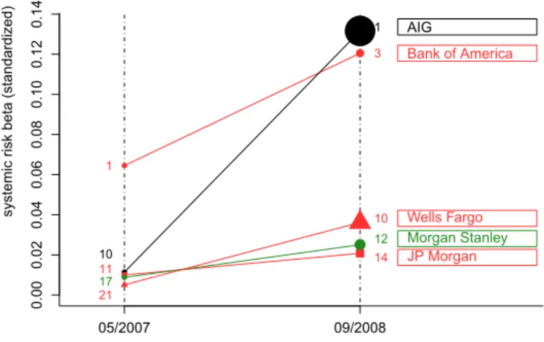
0.00 0.02 0.04 0.06 0.08 0.10 0.12 0.14 05/2007 09/2008
systemic risk beta (standardized)
1 3 Bank of America 10 1 AIG 11 14 JP Morgan 17 12 Morgan Stanley 21 10 Wells Fargo
Figure 2: Systemic relevance of five exemplary firms in the U.S. financial system at two time points before and at the height of the financial crisis, 2008. Systemic relevance is measured in ”systemic risk betas” quantifying the marginal increase of the VaR of the system given an increase in a bank’s VaR while controlling for the bank’s pre-identified risk drivers. All VaRs are computed at the 5% level and are by definition positive. We depict respective “standardized” versions of the systemic risk beta representing the total effect on systemic risk induced by individual VaRs. Connecting lines are just added to graphically highlight changes between the two time points but do not mark real evolutions. The size of the elements in the graph reflects the size of the VaR of the respective company at each of the two time points. We use the following scale: the element isk·standard size with k = 1 for V aR ≤ 0.05, k = 1.5 for V aR ∈ (0.05,0.1], k = 2 for
V aR ∈(0.1,0.15],k = 3forV aR ∈(0.2,0.25]andk = 5.5forV aR ∈(0.65,0.7]. Attached numbers inside the figure mark the position of the respective company in an overall ranking of the 57 largest U.S. financial companies for each of the two time points.
case, the internal risk management of these companies should account for the possible threat induced by the large degree of dependence on others. In particular, assessing their full risk exposure requires network augmented risk measures as our VaR with preselected network risk drivers. The highest attention of supervision authorities should be attracted by firms which mainly act as risk drivers for others in the system. These contain firms in the center of the network which appear as “too interconnected to fail”, but even more so, large depositories at the boundary which drive a small number of firms in the cen-ter of the system. While the systemic risk network yields qualitative information on risk channels and roles of companies within the financial system, estimates of systemic risk betas allow to quantify the resulting individual systemic relevance and thus complement the full picture. Ranking companies based on (standardized) systemic risk betas shows that large depositories are particularly risky. After controlling for all relevant network
effects, they have the overall strongest impact on systemic risk and should be regulated accordingly. Confirming general intuition, time evolutions of (standardized) systemic risk betas indicate that most companies’ systemic risk contribution sharply increases during the financial crisis. These effects are particularly pronounced for firms, such as, e.g., AIG, which indeed got into financial distress during the crisis and are clearly (ex post) iden-tified as being systemically risky by our approach. Figure 2 exemplarily illustrates the evolutions of their marginal systemic contributions – as reflected by systemic risk betas – as well as their exposure to idiosyncratic tail risk – as quantified by their VaR. A de-tailed pre-crisis case study confirms the validity of our methodology as firms such as, e.g., Lehman Brothers are ex-ante identified as being highly systemically relevant. It is well-known that their subsequent failure has indeed had a huge impact on the stability of the entire financial system. Likewise, the extensive bail-outs of AIG, Freddie Mac and Fannie Mae can be justified given their high systemic risk betas and high interconnectedness by the end of 2007.
Our paper relates to several strands of recent empirical literature on systemic risk con-tributions. Closest to our work is White, Kim, and Manganelli (2010) who propose a bivariate vector-autoregressive system of each company’s VaR and the system VaR. They capture time variations in tail risk in a pure time series setting which does not account for mutual dependencies and network effects. In contrast, our model is more structural as it models tail risk in dependence of economic state variables and network spillovers which automatically account for periods of turbulence when predicting the systemic relevance. Similarly, Adrian and Brunnermeier (2010) build on VaR to a construct systemic risk measure without addressing network interconnections and balance sheet characteristics driving individual risk exposures. Moreover, our paper complements papers which mea-sure a company’s systemic relevance by focusing on the size of potential bail-out costs, such as Acharya, Pedersen, Philippon, and Richardson (2010) and Brownlees and Engle (2011). Such approaches cannot detect spillover effects driven by the topology of the risk network and might under-estimate the systemic importance of small but very intercon-nected companies. Moreover, while Brownlees and Engle (2011) study the situation of an individual firm given that the system is under distress, we investigate the reverse relation and measure the effect on the system given an individual firm is in financial trouble. In
the same way, we also complement macroeconomic approaches taking a more aggregated view as, e.g., the literature on systemic risk indicators (e.g., Segoviano and Goodhart, 2009, Giesecke and Kim, 2011) or papers on early warning signals (e.g., Schwaab, Koop-man, and Lucas, 2011, and KoopKoop-man, Lucas, and Schwaab, 2011).
The remainder of the paper is structured as follows. In Section I, we briefly explain the modelling idea and the data. Section II describes the model and estimation procedure for individual companies’ VaRs, before presenting results on the financial network structure. Section III discusses the second stage, the system VaR model, including estimation pro-cedure, inference method and empirical results. In Section IV, we robustify and validate our results by presenting a case study of five large financial institutions that were affected by the financial crisis, and try to predict their distress and systemic relevance using only pre-crisis data. Section V concludes.
I. A Framework for Measuring Systemic Relevance
A. Key Concepts
This section provides a compact overview of the major underlying concepts of how we quantify systemic relevance of a company within the financial system network. It in-troduces major underlying concepts, illustrates how the different steps of the empirical analysis are linked to each other and thus outlines the remainder of the paper. Studying the dependence between systemic risk and firm-specific risk requires modeling relations in the (left) tails of respective asset return distributions, rather than in the center. This is in sharp contrast to a correlation analysis detecting only dependence in mean returns and being inable to quantify spillovers in situations of financial distress.
We consider a stress-test-type scenario for measuring how changes in individual company-specific risk affect the risk of failure of the entire system given the underlying network topology. Therefore, our model does not aim at being structural and building on a general equilibrium framework, but is of reduced form allowing to capture the fullpartialeffect
for a specific company as its systemic risk contribution. Relevant underlying network linkages between tail risks of firms in the system are identified in a first step and crucially determine each company’s tail risk drivers.
We measure systemic risk as the Value at Risk (VaR) of the system returnXs
condi-tional on externalitiesB.5 Then, systemic risk at timet is defined as the system’s loss
position occurring with probabilitypgiven externalitiesB, i.e.,
Pr(−Xts≥V aRsp,t) = Pr(Xts ≤Qsp,t) =p . (1)
Accordingly, Qs
p,t := Qp(Xs|B = Bt) = Qsp(Bt) corresponds to the conditional p
-quantile ofXs. The system VaR is defined using the convention thatV aRp,ts =V aRsp(Bt) =
−Qs
p,t, such that the VaR is non-negative and a higher VaR indicates higher risk as a
func-tion ofB. The setBcontains macroeconomic variables (as specified below), but also tail risk measures of other financial companies. Obviously, due to strong interconnections, the sum of individual tail risks may substantially differ from overall system tail risk. To quantify the full partial effect of changes in the tail risk of an individual institution on the tail risk of the financial system, we incorporate the tail risk of the specific company in the vector of explanatory variablesBin (1) and quantify its marginal effect on the system VaR.
In this context, we have to overcome several difficulties. First, the tail risk of a com-panyiis not directly observable, but has to be estimated, e.g., by the company-specific conditional Value-at-RiskV aRi
q,t =V aRqi(Wt). For statistical inference, discussed later
in the paper, this makes a difference as we have to account for the fact that these vari-ables are pre-estimated leading to nonstandard (increased) confidence intervals. We define V aRi
q(W)analogously to (1) asV aRiq,t = V aRiq(Wt) = −Qiq,t, whereQiq,t =Qiq(Wt)
is the conditionalq-quantile of company i’s return Xi conditional on characteristics W
observed int. The setWt= (1,Mt−1,E−ti,C i
t−1, Xti−1)contains the the possibletail risk
driversof firmiconsisting of macroeconomic state variablesMt−1, lagged firm-specific
characteristics Cit−1, its lagged return Xti−1, and loss exceedances of other companies,
5The system return is defined as the value-weighted average return of a much larger number of
Et−i. The loss exceedance of a firm j is defined asEtj = Xtj1(Xtj ≤ Qˆj0.1), whereQˆ0.1
is the10% sample quantile of firm j’s return. Hence, by construction, company j only affects companyiif the former is under pressure which naturally captures dependencies between tail risks of companies. Correspondingly, E−ti = (Etj)j6=i collects the loss
ex-ceedances of all firms apart from companyiitself. While firm-specific variables, such as leverage or maturity mismatch can be controlled by the bank itself and can thus be seen as ”internal” risk factors, macroeconomic state variables, such as credit spreads or liquidity spreads, and spillovers from other firms under distress are exogenous risk drivers the bank is exposed to.
DefineVt= (1,Mt−1,VaR−qi(Wt))containing the macroeconomic state variables as well as the VaR levels of all other companies butiin the system. Then,Bt is the vector
(Vt, V aRiq(Wt))and the so-calledsystemic risk betais the total marginal effect of firm
i’s tail risk on the system tail risk, ∂V aRs
p(Vt, V aRiq(Wt))
∂V aRi q(Wt)
=βp,qs|i. (2)
The systemic risk beta can be itself varying as it is parameterized in terms of time-varying firm-specific characteristics. This has been suppressed for ease of notation in (2). Systemic risk betas and corresponding rankings comparing the systemic relevance of in-dividual companies are analyzed in Section III.
The second and major difficulty is the question of which risk drivers out of the full sets
VandWare essential to be included in order to measureβp,qs|i unbiasedly while keeping
the model parsimonious and thus tractable. Indeed, not all companies are similarly and/or significantly affected by all characteristics and all other firms contained in V and W. Hence, selecting the statisticallyrelevant risk drivers for each companyi determinesi -specific characteristicsV(i) and W(i) conditional on which the system VaR is linked to
V aRi. Thus it is sufficient if the reduced form model (2) forβs|i
p,q only depends onV(i)
andW(i). Identifying the relevant V(i) andW(i), amounts to a model selection problem
for the tail risk of firmiwhich can be solved with an appropriate statistical penalization technique. In particular, we provide a data-driven way to (pre-)select relevant variables
affectβp,qs|i in the equation (2) for the system VaR and should thus be contained inV(i). The
model selection step is not only necessary to keep the model parsimonious but also allows to uncover underlyingrelevanttail risk dependencies between companies. Ignoring these spillover effects would lead to a biased measure of systemic risk contribution. Moreover, depicting all relevant risk connections between all firms in the system, results in a network graph for systemic risk which contains valuable regulatory information on potential risk channels and specific roles of companies as risk transmitters and/or recipients. Since the identification of such network effects has to be performedbeforesystemic risk betas can be estimated, we present this analysis in Section II before we focus on the estimation of systemic risk betas in Section III.
B. Data
Our analysis focuses on publicly traded U.S. financial institutions. The list of included companies in Table I (see Appendix A) comprises depositories, broker dealers, insurance companies and Others.6 We use publicly available market and balance sheet data for our assessment of systemic relevance. This is a solid basis for transparent regulation since timely access on detailed information of connections between firms’ assets and obliga-tions, is very difficult and expensive to obtain – even for central banks. Daily equity prices are obtained from Datastream and are converted to weekly log returns. To account for the general state of the economy, we use weekly observations of lagged macroeconomic vari-ablesMt−1 as suggested and used by Adrian and Brunnermeier (2010) (abbreviations as
used in the remainder of the paper are given in brackets):
(i) the implied volatility index, VIX, as computed by the Chicago Board Options Ex-change (vix),
(ii) a short term ”liquidity spread”, computed as the difference of 3-month collateral repo rate (available on Bloomberg) and the 3-month Treasury bill rate from the Federal Reserve Bank of New York (repo),
(iii) the change in the 3-month Treasury bill rate (yield3m),
6Companies are distinguished according to their two-digit SIC codes, following the categorization in
(iv) the change in the slope of the yield curve, corresponding to the spread between the 10-year and 3-month Treasury bill rate (term),
(v) the change in the credit spread between BAA rated bonds and the Treasury bill rate (both at 10 year maturity) (credit),
(vi) the weekly equity market return from CRSP (marketret),
(vii) the one-year cumulative real estate sector return, computed as the value-weighted average of real estate companies available in the CRSP data base (housing).
Moreover, to capture characteristics of individual institutions predicting a bank’s propen-sity to become financially distressed,Cit−1, we follow Adrian and Brunnermeier (2010) and use
(i) leverage, calculated as the value of total assets divided by total equity (in book values) (LEV),
(ii) maturity mismatch, measuring short-term refinancing risk, calculated as short term debt net of cash divided by the total liabilities (MMM),
(iii) market-to-book value, defined as the ratio of the market value to the book value of total equity (BM),
(iv) size, defined by the logarithm of market valued total assets (SIZE), (v) equity return volatility, computed from daily equity return data (VOL).
Balance sheets are only available on a quarterly basis and are published on fixed dates (December 31, March 31, June 30 and September 30), while calender weeks start dif-ferently every year. As our analysis builds on weekly frequencies, we interpolate the quarterly data to a daily level using cubic splines, and then aggregate them back to the corresponding calendar weeks. As an illustration, Figure 4 shows the interpolated quar-terly maturity mismatch times for Wells Fargo. We focus on 57 financial institutions for which data is available during the period from beginning of 2000 to end of 2008, resulting into 467 weekly observations on individual returns, macroeconomic factors and individ-ual characteristics (after interpolation). The system return is chosen as the return on the
financial sector index provided by Datastream. It is computed as the value-weighted av-erage of prices of 190 US financial institutions.
Focusing only on those companies for which a maximum of observations is avail-able yields a higher precision of estimates, however, has the drawback that particularly firms which defaulted during the financial crisis 2007-2009 are excluded from the anal-ysis. Therefore, to validate and robustify our approach, we re-estimate the model over a sub-period ending before the financial crisis and include the investment banks Lehman Brothers and Merrill Lynch that were massively affected by the crisis. This ”case study” provides an ex-ante assessment of companies which ex post have been identified as sys-temically relevant and is given in Section IV.
II. A Systemic Risk Network
A. Network Model and Structure
We assume that the VaR of firmifollows a structural model based on those characteris-ticsW(i) which are relevant for companyi. In particular, in a pre-step, these individual
tail risk driversW(i) are selected out of lagged macroeconomic state variables,Mt−1,
re-turns of other distressed companies in the system,E−ti, lagged firm-specific characteristics
Cit−1, thei-specific lagged return,Xti−1, and an intercept. Depicting all connections be-tween all firms and respective companies contained in their set of relevant tail risk drivers produces the corresponding network graph of systemic risk.
A model forV aRi based on economic state variables as well as loss exceedances by
construction automatically adjusts and prevails even in distress scenarios under shocks in externalities. This is a clear advantage compared to pure reduced form time series approaches (cp. e.g. White, Kim, and Manganelli, 2010, and Brownlees and Engle, 2010). For simplicity, we take the underlying model for eachV aRi
qas linear,
The coefficients in the model are specific to the considered quantilequnderlying the VaR. In the following, we describe how to statistically selectW(i)for each firmiand
pro-vide an appropriate estimation technique for the coefficientsξip. Results for econometric inference are non-standard as consistency and standard errors are affected by the pre-selection step and significance tests in quantile relations require backtesting techniques. We summarize the main results in the text, but provide more technical details in the ap-pendix.
B. Identification of Tail Risk Drivers and Estimation
For each firmiin the system, we jointly observe(Xi
t,Wt)at all time pointst= 1, . . . , T,
in the sample with theK-vector of all possible risk driversWt= (1,Mt−1,X−ti,C i
t−1, Xti−1).
According to (1), the firm-specific conditional V aRi
q,t at level q and time point t is
de-fined as the negative conditional q-quantile of Xi given W(ti). Thus, at a specific time pointt∈[0, T], the structural linear model (3) for the VaR corresponds in the quantile to
Xti =−W(ti)0ξqi +εit, for Qq(εit|W
(i)
t ) = 0. (4)
If we knew thei-relevant risk drivers W(i) selected out of W, then, estimates ξbi
q of ξ i q
could be obtained according to standard linear quantile regression (Koenker and Bassett, 1978) by minimizing 1 T T X t=1 ρq Xti+W(ti)0ξiq (5)
with loss functionρq(u) =u(q−I(u < 0)), where the indicatorI(·)is 1 foru < 0and
zero otherwise, and
[
V aRiq,t =W(ti)0bξ
i
q . (6)
However, the relevant risk driversW(i) for firm i are unknown and must be determined fromW in advance. Model selection is not straightforward in the given setting as tests on the individual significance of single variables do not account for the (possibly high) collinearity between the covariates. Moreover, sequences of joint significance test have too many possible variations to be easily checked in case of more than 60 variables. Since
alternative model selection techniques, like BIC or AIC, are not available in a quantile setting, we choose the relevant covariates in a data-driven way by employing a statis-tical shrinkage technique known as the least absolute shrinkage and selection operator (LASSO). LASSO methods are standard for high-dimensional conditional mean sion problems (see Tibshirani, 1996), and recently have been adapted to quantile regres-sion by Belloni and Chernozhukov (2011). Accordingly, we run anL1-penalized quantile
regression and calculate for a fixed individual penalty parameterλi ∈[0,1],
e ξiq =argminξi 1 T T X t=1 ρq Xti+W 0 tξ i +λi p q(1−q) T K X k=1 ˆ σk|ξki|, (7)
withWt = (Wt,k)Kk=1, σˆk = T1 PTt=1(Wt,k)2 and the loss function ρq given by (5) (see
Belloni and Chernozhukov, 2011). The underlying principle is to select relevant regres-sors according to the magnitude of their respective coefficients (scaled by the regressor’s variation). Regressors are then eliminated if their shrunken coefficients are at (or close to) zero. Here, we eliminate all firms inWwith marginal effects|eξi|being in absolute terms below a thresholdτ = 0.0001 and keep only theK(i)relevant regressorsW(i). Hence, LASSO de-selects those regressors contributing only little variation. As all coefficients eξ
i
qare generally downward biased in finite samples because of the additional penalty term
in 7, we then re-estimate the unrestricted model (5) withW(i)to obtain final estimatesξbi
q.
This post-LASSO step produces superior finite sample estimates of coefficientsξiq. For more details, see the Appendix.
The selection of relevant risk drivers via LASSO crucially depends on the choice of the company-specific penalty parameterλi. The largerλi, the more regressors are eliminated.
Conversely, in case ofλi = 0, we are back in the standard quantile regression setting (5) without any de-selection. Accounting for possible serial dependencies in risk driversWt,
we determineλi in a data-driven way following a bootstrap type procedure as suggested by Belloni and Chernozhukov (2011):
Step 1 TakeT iid draws fromU[0,1]independent ofW1, . . . ,WT denoted asU1, . . . , UT.
Conditional on observations ofW, calculate the corresponding value of the random variable, Λi =T max 1≤k≤K 1 T T X t=1 Wt,k(q−I(Ut≤q)) ˆ σk p q(1−q) .
Step 2 Repeat step 1 for B=500 times generating the empirical distribution ofΛi condi-tional onWthroughΛi
1, . . . ,ΛiB. For a confidence levelα ≤1/K in the selection,
set
λi =c·Q(Λi,1−α|Wt),
whereQ(Λi,1−α|W
t)denotes the(1−α)-quantile ofΛi givenWtandc≤2is a
constant.
The choice ofαis a trade-off between a high confidence level and a corresponding high regularization bias from high penalty levels in (7). As in the simulation results in Belloni and Chernozhukov (2011), we choose α = 0.1, which suffices to get optimal rates of the post-penalization estimators below. Finally, the parameter c is selected in a data-dependent way such that the fit ofV aRi is optimized. The latter is evaluated in terms of
its best backtesting performance according to the procedure described below.
C. Model Validation by Backtesting
We evaluate the adequacy of the VaR estimates by quantifying their in-sample predictive ability. This procedure is an alternative to (infeasible) sequential testing procedures on the joint significance of explanatory variables and, moreover, yields a data-driven way to selectcin the LASSO algorithm. In particular, we consider a VaR model as being inade-quate if it fails to produce a sequence of independent VaR exceedances over the considered time period. This is formally tested using a likelihood ratio version of the dynamic quan-tile (DQ) test developed in Engle and Manganelli (2004). Berkowitz, Christoffersen, and
Pelletier (2009) show that the resulting likelihood ratio test has superior size and power properties compared to competing VaR backtesting methods.
For each institutioni, we measure VaR exceedances asIti ≡I(Xti <−V aRi
q,t). If the
chosen model is correct, then,
E[Iti|Ωt] =q , (8)
whereΩtis the information set up tot. The VaR is estimated correctly, if independently
for each day of the covered period, the probability of exceeding the VaR equalsq. Similar to Engle and Manganelli (2004), Kuester, Mittnik, and Paolella (2006) and Taylor (2008), we include a constant, three lagged values ofIt and the current VaR estimate in the
in-formation setΩt. Then, condition (8) can be checked by estimating a logistic regression
model
Iti =α+A0tθ+Ut,
with covariatesAt = (Iti−1, Iti−2, Iti−3,V aR[
i t−1)
0. Denote byI¯i the sample mean of the
binary responseIi
tand defineFlog(·)as the cumulative distribution function of the logistic
distribution. Then, under the joint hypothesis
H0 : α=qandθ1 =· · ·θ4 = 0,
we find the asymptotic distribution of the corresponding likelihood ratio test statistic as
LR =−2(lnLr−lnLu) a
∼χ25 . (9)
Here, lnLu = Pnt=1[ItiFlog(α+At0θ) + (1−Iti) ln (1−Flog(α+A0tθ))] is the
unre-stricted log likelihood function which underH0 simplifies tolnLr =nI¯iln(q) +n(1−
¯
Ii) ln(1−q).
The company-specific outcomes of this test are used to choose the parametercin the LASSO procedure in a data-driven way. In particular, cis chosen such that thep-value associated with (9) for the correspondingly selected model is maximized. This
automati-cally ensures that the LASSO-selected risk drivers for each firm yield optimal in-sample predictions of idiosyncratic tail risk.7
D. Idiosyncratic Risks and Systemic Risk Networks: Empirical
Find-ings
D.1. Idiosyncratic Tail Risks
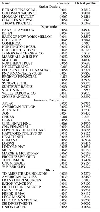
Table II reports the outcomes of the back-testing procedure for the LASSO-selected indi-vidual VaR specifications of all 57 financial companies in our sample. We chooseq=0.05, i.e., focus on the 95%-quantile of the loss distribution.8 All selected models provide good
in-sample fits with mostp-values being well above 0.5. Also the coverages are very close to the nominal level of5% indicating that the estimated V aR[i series capture company-specific tail risks very well.
For the sake of brevity, we do not report all individual VaR regressions but show ex-emplaryV aRi (post-)LASSO regressions for companies representing the four branches
of depositories, insurances, brokers and others in Tables III and IV. It turns out that the LASSO-selected risk drivers significantly differ across companies. Not surprisingly, this is particularly true for the individually selected loss exceedances of other companies com-prising the risk network discussed below. For example, the selected drivers determining the VaR of Goldman Sachs (GS) include, on the one hand, loss exceedances of its biggest competitor, Morgan Stanley (MS) and the insurance company American International Group (AIG). Likewise, Morgan Stanley is driven by the tail risk of many other big com-panies. Conversely, AIG is influenced by only a few other companies including, however, among others, the mortgage company Freddie Mac (FRE). This risk spillover is highly plausible given the evidence from the financial crisis 2008 and is discussed in more detail 7In rare cases, however, the resulting selected model is too small, in the sense that only macroeconomic
variables are included. Then, the system VaR regression cannot be performed, because both the individual VaR and the system VaR are linear combinations of the same variables inducing perfect multi-collinearity. In such cases, we decrease the factorcuntil the most relevant (additional) risk driver is included and the resulting regressor matrix becomes non-singular. In their empirical example, Belloni and Chernozhukov (2011) apply a similar adjustment procedure.
below. Note that nearly all loss exceedances have the expected signs: The greater the loss of other companies (i.e., the more negative their returns falling below the10% quan-tile), the higher the VaR and thus the potential loss of the firm under consideration. The company-specific accounting variables as well as the macroeconomic state variables enter the regressions mostly with positive coefficients. Particularly, leverage, implied market volatility (represented by the VIX) as well as real estate sector returns positively affect companies’ tail risk. The latter reflect firm’s sensitivity to rising housing prices which was one of the major causes for the financial crisis in 2008.
Summary statistics of the estimated VaR time series are given in Table V. We observe a substantial variation of VaRs over the cross-section of the sample as well as over time. The reported quantiles of the VaR realizations indicate that company-specific tail risks, i.e., the magnitude of potential losses, strongly vary over time. In fact, for nearly all companies the highest VaRs and thus the highest realizations of idiosyncratic risk are observed during the financial crisis in 2008.
D.2. The Systemic Risk Network
The individually selected loss exceedances of other companies as tail risk drivers for each firm determine the underlying network of risk spillovers. An overview of the identified tail risk connections between all companies is provided in Table VI. We observe that the number of risk connections substantially vary over the cross-section of companies. While some firms such as, e.g., Morgan Stanley, American Express as well as Bank of New York Mellon, are strongly inter-connected and receive substantial tail risk from other companies, there are institutions for which no network effects can be identified at all. These firms are apparently not significantly influenced, but can themselves still act as risk drivers for others.
In order to effectively summarize and to depict the identified risk connections and directions, we graphically present the entire network of companies in Figure 5. Taking all firms as nodes in such a network, there is an influence of firmj on firmi, ifEjis selected
as a relevant risk externality of firmi inV aRi
q. In particular, ifEj is part of W
k-th component, then the corresponding coefficientξi q,kinξ
i
qdelivers the thickness of the
arrow from firmj to firmi in the network graph. If Ej is not selected as relevant risk driver of firmi, there is no arrow from firmj to firmi. Building the network of relevant spillover effects in such a way does not require the relations between companies to be symmetric. This very much corresponds to empirical evidence, as, e.g., Bank of America might strongly influence a small depository, but vice versa there is no direct significant effect. Moreover, note that dependencies between (extreme) quantiles reflect spillovers in
possiblelosses (occurring with probabilityq) but not necessarily in actually realized ones. We identify four major groups of firms: The first category contains companies with only very few incoming arrows but numerous outgoing ones. These are companies whose potential failure might affect many others but, conversely, which are themselves relatively unaffected by the distress of other firms. We associate these relations with rather ”one-sided” network dependencies. Companies belonging to this group are originators of risk spillovers. Hence, their failure can induce substantial risks of failure of the entire sys-tem. Therefore, these firms should be particularly monitored by regulatory authorities. These are, e.g., Bank of America (BAC), Citigroup (C), Freddie Mac (FRE), Charles Schwab Corporation (SCHW), MBIA (MBI), Unum Group (UNM) and Hartford Finan-cials (HIG). Bank of America and Citigroup are among the top five largest banks in the U.S. Financial distress of these banks obviously has wide-spread consequences. On the other hand, these banks are sufficiently large and own-standing not to be severely affected by the distress of others. Freddie Mac, one of the two largest U.S. mortgage companies, reveals spillovers particularly to large insurance companies such as AIG and MBIA who hold significant positions in mortgage backed securities. These relationships have been one of the major reasons for the financial crisis 2008. Charles Schwab (SCHW) is one of the largest discount brokers having risk connections to JP Morgan and Morgan Stanley, among others. MBIA, Unum Group and Hartford Financials are large insurance com-panies. Due to investments in mortgage backed securities, MBIA realized severe losses during the financial crisis. Our network graph reveals a corresponding dependence on Freddie Mac and shows that MBIA itself affects many other firms.
The second group consists of companies which are strongly interconnected with many other firms. These are Morgan Stanley (MS) and JP Morgan (JPM), belonging to the largest banks in the U.S., Fannie Mae (FNM), the main competitor of Freddie Mac, Amer-ican Express (AXP), one of the biggest financial service companies, as well as the insur-ance company Lincoln Financial Corporation (LNC). These firms are strongly imbedded in the system and thus are both producers and recipients of tail risk. In several cases, these companies amplify tail risk spillovers by further disseminating risk into new channels. A prominent example is Morgan Stanley which is placed in the center of the network and transports risk in many directions. In particular, Morgan Stanley disseminates spillovers from Bank of America which makes the latter itself deeply interconnected. Due to their role as risk distributors such companies are systemically risky and should be supervised on a regular basis.
The third group contains companies which do not serve as major risk producers but are themselves potentially affected by many other institutions. An interesting example is the Bank of New York Mellon (BK) revealing substantial risk input. This is illustrated in Figure 3 depicting the specific role of Bank of New York in the systemic risk net-work. The bank receives risk spillover from many other institutions including several large depositories and broker dealers. This is due to the fact that it serves as one of the major clearing banks in the U.S. Accordingly, its risk increases as soon as its large corpo-rate customers become financially distressed. Further examples are Allstate Corporation (ALL), the second-largest personal lines insurer in the U.S., and Cincinnati Financial Cor-poration (CINF), a company for property and causalty insurance. Finally, we identify a group of companies revealing strong risk connections with only very few other firms. Ex-amples of these predominantly bilateral dependencies are connections between Morgan Stanley and Citigroup, Freddie Mac and Fannie Mae as well as between Goldman Sachs and JP Morgan.
Distinguishing between these four industry groups, we observe that depositories tend to be less involved than insurance companies. Most insurances are placed in the center of the network graph and thus serve as both risk recipients and transmitters. The same is true for broker dealers which tend to be even stronger interconnected. As discussed
Figure 3: Schematic subgraph of the risk network of the U.S. financial system highlighting the role of the Bank of New York Mellon (BK) in bold as a major clearing house. For simplicity, ar-rows only mark risk spillovers effects without referring to their respective size, otherwise they are as defined in Figure 1. Likewise, the colors are defined as in Figure 1. Arrows are only displayed in this figure if pointing towards BK. The graph only contains firms with a direct influence on BK (in the shaded ellipsoid closest to BK) and those which might influence BK on a "second level" (in the larger ellipsoid). A list of their abbreviations is contained in Table I.
above, an extreme example is Morgan Stanley which is heavily involved and imports as well as exports tail risk in many directions. In contrast, several depositories are placed at the edge of the network and tend to serve rather as risk transmitters than recipients. Typical examples are Bank of America and Citigroup which are, however, themselves strongly connected to risk distributors which further disseminate tail risk.
Figure 6 shows a subset of the network depicting only the risk linkages of Citigroup. The number of possibly affected banks might be used as an indicator of Citigroup’s sys-temic relevance. Holding fixed Citigroup’s tail risk inflow (from LNC and JPM), this ”network tree” graphically presents how financial distress is transmitted through the sys-tem. Figure 7 presents the corresponding network tree for Morgan Stanley. As discussed above, this company shows bi-directional risk connections with numerous other compa-nies. Therefore, in this case, causal interpretations are harder and require to condition on the risk in-flows of several other firms. However, the topology of this sub-network looks quite different than that of Citigroup. The latter has only a few direct connections with
other firms which are, however, further distributed in many other directions in the next layers. Conversely, Morgan Stanley has more neighbors which are directly affected by risk spillovers which are still further multiplied in the second level.
Hence, though a risk network does not allow to quantitatively assess the systemic rel-evance of a financial institution, the degree of firms’ interconnectedness and the specific topology of the network or corresponding sub-networks allows to identify possible risk channels in the system. These interlinkages are central for macroprudential regulation. They reflect the particular role of a firm as risk recipient, transmitter or distributor of tail risk. In this sense, systemic risk networks provide valuable accompanying information for a reduced-form analysis quantifying the marginal effects of individual distress on the system. Such an analysis is performed in the following section.
III. Quantifying Systemic Risk Contributions
A. A Reduced Form Model for Systemic Risk Betas
Our main focus is to provide an accurate but parsimonious measure of the effect of a marginal change in the tail risk of firmion the tail risk of the system given the underlying network structure of the financial system. For an unbiased marginal effect, however, it is sufficient just to control for all firmi-specific risk drivers in a corresponding reduced-form model. Conversely, a fully-fledged structural general equilibrium model is not necessary and, even if correctly specified, would be almost impossible to estimate, given the high-dimensionality and interconnectedness of the financial system on the one hand and data availability on the other. Moreover, variables unrelated to V aRi do not affect firm i’s systemic risk contribution.9 For this reason, we propose estimating systemic risk
con-tributions based on reduced-form models which are specific for each firmias they only 9See Angrist, Chernozhukov, and Fernández-Val (2006) for a simple Frisch-Waugh-type argument in
control for the i-specific risk drivers. Correspondingly, we estimate the firm-i-specific
systemic risk betaβq,ps|i based on a linear model for the system VaR of the form
V aRp,ts =V(ti)0γps+βp,qs|iV aRiq,t, (10)
where the vector of regressors V(ti) = (1,Mt−1,VaR (−i)
q,t ) includes a constant effect,
lagged macroeconomic state variables and the VaRs of all companies which are identi-fied as risk drivers for firmivia LASSO in Section II.
The systemic risk beta βp,qs|i = βs|i of company i captures the effect of a marginal
change in V aRi
t on V aRst. It can be interpreted in analogy to an inverse asset pricing
relationship in quantiles, where banki’s return quantiles drive the quantiles of the sys-tem given network-specific effects and firm-specific and macroeconomic state variables. Accordingly,
¯
βp,qs|i :=βp,qs|iV aRit (11)
measures the full partial effect of a tail risk increase of bankionV aRs
t. We refer toβ¯ s|i p,q
asstandardizedsystemic risk beta since it allows to cross-sectionally compare systemic risk contributions and to rank banks according to their systemic relevance.
During periods of turbulence, such as crises, not only banks’ risk exposures change but also their marginal importance for the system might vary. We therefore allow βs|i
being time-varying. In particular, time-variation occurs through observable factors Zi
characterizing a bank’s propensity to get in financial distress. Accordingly, βts|i should be interpreted as aconditionalsystemic risk beta. Basingβs|i on lagged characteristics, makes betas and thus corresponding systemic risk rankings predictable which is important for forward-looking regulation. To limit complexity and computational burden of the model, we assume linearity ofβp,q,ts|i inKZ firm-specific distress indicatorsZit−1,
where ηsp,q|i are the parameters driving the time-varying effects. The case of a constant
systemic risk beta is obviously contained as a special case ifηsp,q|i = 0and thus βs
|i
0,p,q =
βp,q,ts|i =βp,qs|i.
We suggest choosingZti as a subset of Cti consisting of the major drivers of a bank’s distress such as size, leverage, and maturity mismatch. As a testable hypothesis, we pos-tulate that these variables do not only affect a bank’s VaR, but simultaneously also drive its marginal systemic relevance. As a consequence, rankings based onβts|idirectly control for size, leverage, and maturity mismatch and do not require any ex-post adjustments for these characteristics. Due to the linearity of (12) we can thus write the quantile model (10) forV aRspwith time-varyingβp,q,ts|i in the following form
V aRsp,t=V(ti)0γsp+β0s|,p,qi V aRiq,t+ (V aRiq,t·Zit−1)0ηsp,q|i . (13)
B. Estimation and Inference
If firm specific VaRs were directly observable, the magnitude and significance ofi-specific systemic risk betas could be directly inferred from the linear quantile regression (13) with the VaR defined by (1). However, note that the regressorsV aRi
tandVaR
(−i)
q,t inV
(i)
are pre-estimated as they arise from the first-step quantile regressions as shown in Section II. Hence, operationalizing (13) withV aR[itandVaRd
(−i)
q,t as generated regressors, yields the
(second step) quantile regression,
Xts =−Vd(i) 0 tγ s p−β s|i 0,p,qV aR[ i q,t−(V aR[ i q,t·Z i t−1) 0 ηsp,q|i +εst, (14) with Qp(εst|V aR[ i q,t,Vbt,Zit−1) = 0 .
With the notationVbt, we stress that some components ofVare pre-estimated asVaRd
(−i)
q,t .
Then, analogously to the first-step regressions in Section II, parameter estimates are ob-tained via quantile regression minimizing
1 T T X t=1 ρp Xts+Vd(i) 0 tγ s p+β s|i 0,p,qV aR[ i q,t+ (V aR[ i q,t·Z i t−1) 0 ηsp,q|i (15)
in the unknown parameters. Consequently, the resulting estimate of the full time-varying marginal effectβb s|i p,qin (12) is obtained as b βp,q,ts|i =βb s|i 0,p,q+Z i t−1 0 d ηp,qs|i (16)
for given valuesZit−1.
SinceV aRiq,tis a function ofW(i), conditional quantile independence in (14) is equiv-alent toQp(εst|W (i) t ,W (−i) t ,Zit−1) = 0whereW (−i) t stacksW (j)
t for all firms relevant for
companyiappearing inVaRd
(−i)
q,t . Hence, with both quantile regression steps being linear,
inserting (3) into (13) yields a full model for the system’s tail risk in observable character-istics. However, direct one-step estimation is only feasible if the choice ofW(i) and thus
VaR(q,t−i) is still determined in a pre-step from individual VaR regressions. Model selec-tion based on the full model ofV aRsin observables is infeasible since correlation effects among the huge number of regressors would produce unreliable results. Furthermore, in-dividual parametersβ0s,p,q|i andηsp,q|i could not be identified without additional identification
conditionQq(εit|W
(i)
t ) = 0, implicitly bringing back the first-step estimation. Therefore
we use two-step estimation even if exact asymptotic confidence intervals are larger than for an (infeasible) single step procedure. In contrast to mean regressions, such results are non-standard in a quantile setting and are therefore provided in detail in the Appendix. In finite samples, however, asymptotic distributions often only provide a poor approxi-mation to the true distribution of the (scaled) difference between the estimator and the true value if sample sizes are not sufficiently large. In case of quantile regressions, this effect is even more pronounced, since valid estimates for the asymptotic variance follow poor non-parametric rates and thus require even larger sample sizes to obtain the same precision.
Therefore, for judging the quality of the estimates βˆp,q,ts|i , we suggest a procedure for testing their significance which is valid in finite samples. In the given setting, we aim at testing for the significance of a systemic risk beta, and/or time-variations thereof. We
adapt a test proposed by Chen, Ying, Zhang, and Zhao (2008) for median regressions to a quantile setting. The test statistic is
ST = min ξs∈Ω0 T X t=1 ρp(Xts−B 0 tξ s)− min ξs∈RdB T X t=1 ρp(Xts−B 0 tξ s), (17)
with the compound vector of all regressors inV aRs, B
t ≡ (V aRit, V aRit ·Z i t−1,V
(i)
t ),
corresponding parameterdB-vectorξs, andΩ0 refering to the constrained set of
parame-ters underH0. The asymptotic distribution ofST involves the probability density function
of the underlying error terms and is not feasible. Furthermore, bootstrappingST directly
would yield inconsistent results. Therefore, we re-sample from the adjusted statistic
ST∗ = min ξs∈Ω 0 T X t=1 wtρp(Xts−B 0 tξ s )− min ξs∈RdB T X t=1 wtρp(Xts−B 0 tξ s ) − T X t=1 wtρp(Xts−B 0 tξˆ s c)− T X t=1 wtρp(Xts−B 0 tξˆ s ) ! , (18)
whereˆξsc denotes the constrained estimate ofξs, and{wt}is a sequence of standard
ex-ponentially distributed random variables, having both mean and variance equal to one. According to Chen, Ying, Zhang, and Zhao (2008), the empirical distribution ofST∗ pro-vides a good approximation of the distribution ofST. Thus, if the test statisticST exceeds
some large quantile of the re-sampling distribution ofST∗, the null hypothesis is rejected. The proposed testing method does not require re-sampling of observations but is en-tirely based on the original sample. This provides significant gains in accuracy in the two-step regression setting as opposed to standard pairwise bootstrap techniques as a fur-ther alternative. A pre-analysis shows that this wild bootstrap type procedure is valid in the presented form as any serial dependence in the data is sufficiently captured by the regressors in the reduced-form relation not requiring block-bootstrap techniques.10
10Pairwise block-bootstrap yields block lengths of one according to the standard procedure of Lahiri
C. Empirical Evidence on Systemic Risk Betas
We estimate systemic risk betas according to (14) with their time variation driven byZi
consisting of a firm’s leverage, maturity mismatch and size. Hence, time-variations of sys-temic risk betas are exclusively due to changes of firm-specific effects. As a consequence, systemic risk contributions of two companies with the same exposure to macroeconomic risk factors and financial network spillovers may be still different as they depend on their balance sheet structures. As in the first-step estimations we choose q = 0.05, i.e., we model the loss which will not be exceeded with 95% probability. For notational conve-nience, we supress the quantile index as we setp=q.
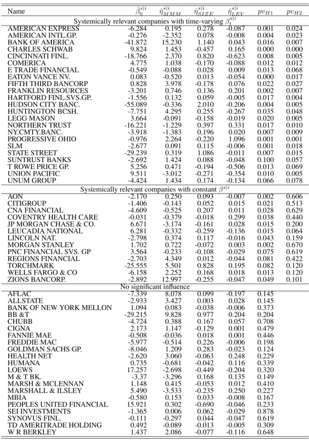
Table VII reports the point estimates forβ0s|i, the constant (marginal) effect ofV aRion
V aRs as well as the parameters associated with the interaction variables,ηsM M M|i , ηSIZEs|i and ηLEVs|i . Note that a positive systemic risk beta indicates that an increase in V aR[i
(expressed as a positive number) induces an increase of the conditional quantile of the negative system return distribution and thus rises the risk of distress of the system.
In order to test whether a company’s systemic relevance is statistically significant, we test its systemic risk beta against zero, i.e.,βts|i = 0. This test requires testing for the joint significance of all variables driving a firm’s marginal impact leading to the hypothesis
H1:β0s|i =ηM M Ms|i =ηsSIZE|i =ηLEVs|i = 0.
If this null hypothesis cannot be rejected, an increase of the company’s possible loss posi-tion, given all economic state variables andi-specific risk inflows from other companies, does not induce a significantly higher potential systemic loss. Accordingly, we consider such a company as not being systemically relevant. To test whether systemic risk betas are time-varying, we test the joint hypothesis
H2:ηM M Ms|i =ηSIZEs|i =ηsLEV|i = 0.
If this hypothesis is not rejected, we re-specify the systemic risk beta as being constant and re-estimate the model without interaction variables. In this case,βts|i =βs|i.
The underlying tests are performed using the wild bootstrap procedure illustrated in Section B based on2,000resamples of the test statistic. The results are reported in form ofp-values in Table VII. According to our test outcomes we distinguish between three groups of companies. In the upper part of the table, we report the estimates of sys-temically relevant companies with time-varying systemic risk betas (i.e., rejecting both hypothesesH1 and H2), while in the middle panel, we show results for firms that are systemically relevant but reveal time-invariant betas (i.e., rejectingH1 but notH2). Fi-nally, the lower panel contains institutions that are not significantly systemically relevant. The underlying significance level is chosen to be 10% as the number of observations is not very large relative to the number of regressors, in particular, when considering the two-stage regression setting.
As shown by Table VII, various companies are systemically not relevant as their marginal contributions to the system’s tail risk are not significant. Confirming the network anal-ysis in Section D.2, most of these companies do not serve as tail risk drivers for other firms. Notable exceptions are the two government-sponsored companies (GSEs) Federal National Mortgage Association (Fannie Mae) and Federal Home Loan Mortgage Cor-poration (Freddie Mac). The latter were massively affected by the financial crisis and were bailed out by Federal Reserve and U.S. Treasury in July 2008. The fact that these companies are not significantly systemically relevant through the entire sample period is obviously due to a structural change in September 2008, when the two GSEs were placed under conservatorship of the U.S. government. To provide deeper insights into such ef-fects, we re-visit the systemic importance of Fannie Mae and Freddie Mac, among others, by explicitly focusing on a periodbefore the crisis in Section IV. Moreover, more than half of all insurance companies are shown to be systemically not relevant. As pointed out by Schich (2009), many of these companies were also not too much affected during the financial crisis 2007-2009 as their investment portfolios mainly contained stocks and bonds rather than mortgage-backed securities.
Overall, the majority of systemically relevant companies are banks. Among the (sig-nificantly) systemically relevant firms, several companies reveal systemic risk betas for which we cannot identify significant time variations in dependence of company-specific
characteristics. Hence, those companies’ marginal contributions to systemic risk are obvi-ously not affected by their size, leverage, and maturity mismatch. Examples are Regions Financial, Zions Corporation and JP Morgan with comparably high systemic risk betas across time and the cross-section of institutions. In contrast, for many other firms, we indeed find significant time-varying marginal effects on systemic risk. As reported by Table VII, the coefficients associated with maturity mismatch, size and leverage driving the time variation in systemic risk betas are dominantly positive. Thus marginal systemic relevance increases if a company becomes larger and is exposed to higher idiosyncratic risk.11
Important examples of companies with highly significant and time-varying systemic risk betas are Bank of America and AIG. AIG was among the largest issuers and holders of credit default swaps (CDS) and other credit securitization derivatives before the crisis. Its obviously strong exposure to mortgage default risks is reflected by a strong dependence to Freddie Mac as reflected in the network graph in Figure 5. Consequently, AIG faced tremendous write-downs in 2008, and received rescue packages amounting to USD 150 billion (see Schich, 2009). Our finding of AIG being systemically relevant quantitatively complements our results on AIG’s network dependencies (see Section D.2) revealinghow
AIG’s tail risk affects the financial system. In fact, AIG produces risk spill-overs to Gold-man Sachs and Morgan Stanley, among others. As discussed above, particularly Morgan Stanley is deeply interconnected and serves as multiplier of tail risk. Its strong link to AIG is obviously a major channel for the formation of systemic risk. The upper part of Figure 8 depicts the AIG-specific estimates of βts|i and V aRi
t as well as the product
thereof,β¯ts|i, measuring the standardized systemic risk contribution. We observe that sys-temic risk betas significantly vary over time and particularly increase during the financial crisis. Likewise, the firm’s VaR strongly increases during the crisis period reflecting also severe idiosyncratic risk. Naturally the same pattern is revealed by the standardized sys-temic risk betaβ¯ts|i. Though on first sight, it seems to be counter-intuitive that towards the end of the sample, bothβˆts|i andbβ¯
s|i
t decrease, this pattern is explained by the fact that
11However, because of multi-collinearity between these variables, the interpretation of individual
coeffi-cients is rather difficult. Therefore, it is more reasonable to analyze their total impact on systemic risk betas resulting in variations over time. This analysis is performed in Section D.
the rescue packages from the Federal Reserve were issued in September 2008. This step signficantly reduced the risk of both AIG’s and the entire system’s failure.
Another example is Bank of America. As discussed in Section D.2, Bank of America serves as a tail risk driver for others but is not a tail risk recipient. Our estimates indicate that its risk channels, particularly to Morgan Stanley, are systemically critical. Figure 8 shows that Bank of America’s systemic risk beta has been relatively stable before the financial crisis but significantly dropped after the issuance of the Federal Reserve’s rescue packages. Nevertheless, its VaR and thus its standardized systemic risk beta strongly increased during the crisis and particularly thereafter. The average standardized systemic risk beta computed over the entire sample period indicates that a 1% increase of the VaR induces a8.7basis point increase of the system VaR.
To cross-validate our findings with external evaluations of banks’ systemic importance we refer to the Supervisory Capital Assessment Program (SCAP) conducted by the Fed-eral Reserve in spring 2009. The 19 largest bank holding companies went through com-prehensive investigations resulting in estimates of a potential lack of capital buffer to cover their risks under an adverse macro scenario. In this analysis, detailed information on balance sheet positions were used, including data which are not publicly available. For details, see Federal Reserve System (2009). Since the SCAP took place right after the end of our sample period, it is insightful to compare the outcomes with our results and to check whether our model, which uses more aggregated data, is still able to detect the systemic riskiness of those companies that, according to the SCAP, faced capital short-age in the stress test scenario. Indeed, the financial institution with the biggest potential lack of capital buffer according to the SCAP, Bank of America, is among our systemi-cally relevant companies, with a highly significant systemic risk beta βts|i. In addition, with Citigroup, FifthThird Bancorp, Morgan Stanley, PNC, Regions Financial, SunTrust Banks and Wells Fargo we identify all eight banks contained in our database12 which,
according to the SCAP results, were threatened by financial distress under more adverse market conditions. This becomes even more evident in light of the systemic risk rankings as shown in Section D.
12Due to a lack of data, we cannot include KeyCorp and GMAC in our analysis which also have been