University of Nebraska - Lincoln
University of Nebraska - Lincoln
DigitalCommons@University of Nebraska - Lincoln
DigitalCommons@University of Nebraska - Lincoln
CSE Technical reports
Computer Science and Engineering, Department
of
2006
On Reoptimizing Multi-Class Classifiers
On Reoptimizing Multi-Class Classifiers
Kun Deng
University of Nebraska-Lincoln
Chris Bourke
University of Nebraska-Lincoln
Stephen Scott
University of Nebraska-Lincoln, [email protected]
Robert E. Schapire
Princeton University
N. V. Vinodchandran
University of Nebraska-Lincoln
Follow this and additional works at: https://digitalcommons.unl.edu/csetechreports
Part of the Computer Sciences Commons
Deng, Kun; Bourke, Chris; Scott, Stephen; Schapire, Robert E.; and Vinodchandran, N. V., "On Reoptimizing Multi-Class Classifiers" (2006). CSE Technical reports. 12.
https://digitalcommons.unl.edu/csetechreports/12
This Article is brought to you for free and open access by the Computer Science and Engineering, Department of at DigitalCommons@University of Nebraska - Lincoln. It has been accepted for inclusion in CSE Technical reports by an
On Reoptimizing Multi-Class Classifiers
∗
Kun Deng
†Chris Bourke
†Stephen D. Scott
†Robert E. Schapire
‡N. V. Vinodchandran
†December 5, 2006
Abstract
Significant changes in the instance distribution or associated cost function of a learning problem require one to reoptimize a previously learned classifier to work under new conditions. We study the problem of reoptimizing a multi-class classifier based on its ROC hypersurface and a matrix describing the costs of each type of prediction error. For a binary classifier, it is straightforward to find an optimal operating point based on its ROC curve and the relative cost of true positive to false positive error. However, the corresponding multi-class problem (finding an optimal operating point based on a ROC hypersurface and cost matrix) is more challenging and until now, it was unknown whether an efficient algorithm existed that found an optimal solution. We answer this question by first proving that the decision version of this problem is NP-complete. As a complementary positive result, we give an algo-rithm that finds an optimal solution in polynomial time if the number of classesnis a constant. We also present several heuristics for this problem, including linear, nonlinear, and quadratic programming for-mulations, genetic algorithms, and a customized algorithm. Empirical results suggest that under uniform costs several methods exhibit significant improvements while genetic algorithms and margin maximiza-tion quadratic programs fare the best under nonuniform cost models.
Keywords: Receiver Operator Characteristics, classifier reoptimization, multi-class classification.
1
Introduction
We study the problem of re-weighting classifiers to optimize them for new cost models. For example, given a classifier optimized to minimize classification error on its training set, one may attempt to tune it to improve performance in light of a new cost model. Equivalently, a change in the class distribution (the probability of seeing examples from each particular class) can be handled by modeling such a change as a change in cost model. More formally, we are concerned with finding a nonnegative weight vector (w1, . . . , wn) to minimize
m X i=1 c yi,argmax 1≤j≤n {wjfj(xi)} , (1)
given labeled examples{(x1, y1), . . . ,(xm, ym)} ⊂ X × {1, . . . , n}for instance spaceX, a family of confidence
functionsfj:X →R+ for 1≤j≤n, and a cost functionc:{1, . . . , n}2→R+.
This models the problem of reoptimizing a multi-class classifier in machine learning. A machine learning algorithm takes a setS={(x1, y1), . . . ,(xm, ym)} ⊂ X × {1, . . . , n}of labeled training examples and selects
a functionF :X → {1, . . . , n}that minimizes misclassification cost onS, which isPm
i=1c(yi, F(xi)), where
costc(yi, F(xi)) is a nonnegative function measuring the cost of predicting classF(xi) on examplexi whose
∗Preliminary results appeared in Deng et al. (2006).
†Dept. of Computer Science, University of Nebraska, Lincoln, NE 68588-0115, USA, {
kdeng, cbourke, sscott, vinod}@cse.unl.edu
‡Dept. of Computer Science, Princeton University, 35 Olden Street, Princeton, NJ 08540, USA,
Technical Report TR-UNL-CSE-2006-0017, Department of
Computer Science & Engineering, University of Nebraska
true label isyi. For convenience, we will assume that the classifierF is represented by a set of nonnegative
functions fj :X → R+ forj ∈ {1, . . . , n}, wherefj(x) is the classifier’s confidence that x belongs in class
j, and F(x) = argmax1≤j≤n{fj(x)}. Each confidence function fj can be seen as a “base learner” (as in a
one-versus-rest strategy).
An obvious solution would be to simply rerun the base learning algorithm to reoptimize each confidence function fj for the new cost function1. However, this process may be very expensive or even impossible.
Thus, the task before us is to reoptimize F without discarding the family of base learners. As an example, consider the machine learning application of predicting where a company should drill for oil. In this example the set of instancesX consists of candidate drilling locations, each described by a set of attributes (e.g. fossil history of the site, geographic features that quantify how well oil is trapped in an area, etc.). The set of classes could be a discrete scale from 1 to n, where 1 indicates no oil would be found, and n indicates a highly abundant supply. To learn its classifierF, the learning algorithm was given a setS⊂ X × {1, . . . , n} of instance-label pairs as well as a nonnegative, asymmetric cost function c, where c(j, k) measures the cost of money and resources of thinking that an area of classj really was classk. (This function not only indicates the cost of committing excessive resources to an area with too little oil, but also of committing too few resources to an area with abundant oil.) Once the function F is learned and put into practice, it may become the case that the cost function changes from c to c0, e.g. if new technologies in drilling and
shipping of oil emerge. If this happens, then the function F is no longer appropriate to use. One option to remedy this is to discardF and train a new classifierF0 onS under cost function c0. However this may be very resource-consuming since many learning algorithms take extensive time and effort to train. (It may also be impossible if the dataSis unavailable, say due to proprietary restrictions.) In this case the best (or perhaps only) choice is to reoptimizeFbased on a new (possibly smaller) data set. Such problems have been studied extensively (Fieldsend & Everson, 2005; Ferri et al., 2003; Hand & Till, 2001; Lachiche & Flach, 2003; Mossman, 1999; O’Brien & Gray, 2005; Srinivasan, 1999).
For learning tasks with only n = 2 classes, this problem is equivalent to that of finding the optimal operating point of a classifier given a ratio of true positive cost to false positive cost and has a straightforward solution via Receiver Operating Characteristic (ROC) analysis (Lachiche & Flach, 2003). ROC analysis takes a classifierF that outputs confidences in its predictions (i.e. a ranking classifier), and precisely describes the tradeoffs between true positive and false positive errors. By ranking all examplesx∈S by their confidences h(x) from largest to smallest (denoted S ={x1, . . . , xm}), one achieves a set of n+ 1 binary classifiers by
setting thresholds{θi = (h(xi) +h(xi+1))/2,1≤i < m} ∪ {h(x1)−, h(xm) +}for some constant >0.
Given a relative costcof true positive error to false positive error and a validation setS of labeled examples, one can easily find the optimal threshold θ based on S andc (Lachiche & Flach, 2003). To do so, simply rank the examples in S, try every threshold θi as described above, and select the θi minimizing the total
cost of all errors onS.
Though the binary case lends itself to straightforward optimization, working with multi-class problems makes things more difficult. A natural idea is to think of ann-class ROC space having dimensionn(n−1). A point in this space corresponds to a classifier, with each coordinate representing the misclassification rate of one class into some other class2. According to Srinivasan (1999), the optimal classifier lies on the convex
hull of these points. Given this ROC polytope, a validation set, and an n×ncost matrix M with entries c(y,yˆ) (the cost associated with misclassifying a classyexample as class ˆy), Lachiche and Flach (2003) define the optimization problem as finding a weight vectorw~ ≥~0 to minimize (1).
No efficient algorithm is known to optimally solve this problem forn >2, and Lachiche and Flach (2003) speculate that the problem is computationally hard. We present a proof that the decision version of this problem is in fact NP-complete. As a complementary positive result, we give an algorithm that finds an optimal solution in polynomial time (w.r.t. the number of examples, m) when the number of classes n is constant. We also present several new heuristics for this problem, including an integer linear programming relaxation, a sum-of-linear fractional functions (SOLFF) formulation, and a quadratic programming formu-1Equivalently, a change in the class distribution (the probability of seeing examples from each particular class) can be handled by modeling such a change as a change in cost function.
lation as well as a direct optimization of (1) with a genetic algorithm. Finally, we present a new custom algorithm based on partitioning the set of all classes into two metaclasses. This algorithm is similar to that of Lachiche and Flach (2003), but is more efficient. In our experiments, our algorithms yielded several significant improvements both in minimizing classification error and minimizing cost.
The rest of this paper is as follows. In Section 2 we discuss related work. In Section 3 we prove the decision version of this problem (which we call Reweight) is NP-complete and in Section 4 we present an algorithm for producing an optimal solution that is efficient for a constant number of classes. Next, in Section 5 we discuss our heuristic approaches to this problem. We then experimentally evaluate our algorithms in Section 6 and conclude in Section 7.
2
Related Work
The success of binary ROC analysis gives hope that it may be possible to adapt similar ideas to multi-class scenarios. However, research efforts (Srinivasan, 1999; Hand & Till, 2001; Ferri et al., 2003; Lachiche & Flach, 2003; Fieldsend & Everson, 2005) have shown that extending current techniques to multi-class problems is not a trivial task. One key aspect to binary ROC analysis is that it is highly efficient to represent trade-offs of misclassifying one class into the other via binary ROC curves. In addition, the “area under the curve” (AUC) nicely characterizes the classifier’s ability to produce correct rankings without committing to any particular operating point. Decisions can be postponed until a desired trade-off is required (e.g. finding the lowest expected cost).
Now consider the problem of classification in an n-class scenario. A natural extension from the binary case is to consider a multi-class ROC space as having dimensionn(n−1). A point in this space corresponds to a classifier with each coordinate representing the misclassification rate of one class into some other class. Following from Srinivasan (1999), the optimal classifier lies on the convex hull of these points.
Previous investigations have all shared this basic framework (Mossman, 1999; Srinivasan, 1999; Hand & Till, 2001; Ferri et al., 2003; Lachiche & Flach, 2003; Fieldsend & Everson, 2005; O’Brien & Gray, 2005). They differ, however, in the metrics they manipulate and in the approach they use to solve multi-class optimization problems. Mossman (1999) addressed the special case of three-class problems, focusing on the statistical properties of the volume under the ROC surface. This motivated the later work of Ferri et al. (2003), Lachiche and Flach (2003), and O’Brien and Gray (2005). Hand and Till (2001) extended the definition of two-class AUC by averaging pairwise comparisons. They used this new metric in simple, artificial data sets and achieved some success. Ferri et al. (2003) took a different approach in which they strictly followed the definition of two-class AUC by using “Volume Under Surface” (VUS). They were able to compute the bounds of this measure in a three-class problem by using Monte Carlo methods. However, it is not known how well this measure performs in more complex problems.
Fieldsend and Everson (2005), Lachiche and Flach (2003) and O’Brien and Gray (2005) developed algo-rithms to minimize the overall multi-class prediction accuracy and cost given some knowledge of a multi-class classifier. In particular, Fieldsend and Everson approximate the ROC Convex Hull (ROCCH) using the idea of “Pareto front.” Consider the following formulation: letRj,k(θ) be the misclassification rate of predicting
examples from class j as class k. This is a function of some generalized parameter θ that depends on the particular classifiers. For example, θ may be a combination of a weight vector w~ and hypothetical cost matrixM. The goal is to findθthat minimizesRj,k(θ) for allj, kwithj6=k. Consider two classifiersθand
φ. Fieldsend and Everson sayθ strictly dominates φif all misclassification rates for θ are no worse thanφ and at least one rate is strictly better. The set of all feasible classifiers such that no one is dominated by the other forms thePareto front. Fieldsend and Everson present an evolutionary search algorithm to locate the Pareto front. This method is particularly useful when misclassification costs are not necessarily known. More closely related to our work are the results of Lachiche and Flach (2003) and O’Brien and Gray (2005). Lachiche and Flach considered the case when the misclassification cost is known, and the goal is to find the optimal decision criterion that fits the training set. Recall that this can be solved optimally for the binary case. In particular, only one thresholdθ is needed to make the decision for two-class problems. Since there are only m+ 1 possible thresholds for m examples, it is efficient enough to simply test all
possibilities and select the one that gives the minimum average error (or cost). However, the situation is more complicated for multi-class problems. The main obstacle in the multi-class case is that the number of possible classification assignments grows exponentially in the number of instances: Ω(nm).
Lachiche and Flach (2003) formulated the multi-class problem as follows. Suppose the multi-class learning algorithm will output a positive, real-valued functionf : {x1, . . . , xm} × {C1, . . . , Cn} →R+. Here,fj(xi)
gives the confidence that example xi belongs to class j. The decision criterion simply assigns examplexi
to the class with maximum score. Reweighting the classes involves defining a nonnegative weight vector ~
w= (w1, w2, . . . , wn), and predicting the class for an examplexas
h(x) = argmax
1≤j≤n
wjfj(x) .
Sincew~ has only n−1 degrees of freedom, so we can fixw1= 1.
Lachiche and Flach (2003) used a hill climbing heuristic to find a good weight vector w~. In particular, they took advantage of the fact that the optimal threshold for the two-class problem can be found efficiently. For each coordinate in the weight vector, they mapped the problem to a binary problem. The algorithm starts by assigningw1= 1 and all other weights 0. It then tries to decide the weight for one class at a time
as follows. LetSbe the set of labeled examples and letj be the current class for which we want to assign a “good” weightwj. Then the set of possible weights forwj is
max i∈{1,...,j−1}fi(x) fj(x) x∈S .
It is not difficult to see that at any stage there are at most O(|S|) possible weights that can influence the prediction. Thus choosing the optimal weight in this setting can be easily achieved by checking all possibilities. Overall, their algorithm runs in time Θ(nmlogm). Though there is no guarantee that this approach can find an optimal solution, they gave empirical results that it works well for optimizing 1BC, a logic-based Bayes classifier (Lachiche & Flach, 1999).
Although only briefly mentioned by Lachiche and Flach (2003), this ROC thresholding technique is quite extensible to cost-sensitive scenarios. O’Brien and Gray (2005) investigated the role of a cost matrix in partitioning the estimated class probability space and as a replacement for the weights. Assuming thatM is a misclassification cost matrix, an optimal decision criterion would be
h(x) = argmax 1≤j≤n X 1≤k≤n c(j, k) ˆpk(x) .
If ˆpk(x) is a good probability estimate of examplexbelonging to classk, this prediction results in the lowest
expected cost. However, if ˆpk(x) is not an accurate probability estimate, then to ensure optimality, the cost
matrixM has to be altered accordingly. Thus the cost matrixM plays a similar role as the weight vector of Lachiche and Flach (2003) in defining the decision boundary in estimated probability space. O’Brien and Gray (2005) defined several standard operations to manipulate the cost matrix M and proposed the use of a greedy algorithm to find the altered cost matrix (called aboundary matrix).
While the multi-class problem has been studied via heuristics, no one has yet answered the question as to whether this problem is hard, and no one has found efficient algorithms to solve restricted cases of the multi-class problem. Below we provide answers to both of these open questions as well as extend the current literature of heuristics.
3
Hardness
We now prove our hardness result of this problem. For convenience, we use fij to denote fi(xj). We will
show hardness for the uniform cost case, i.e.c(j, k) = 1 whenj6=kand 0 otherwise. This of course implies hardness for any nontrivial cost function.
Definition 1. ProblemReweight
Given: nonnegative real numbersfij (i= 1, . . . , m,j= 1, . . . , n), integersyi ∈ {1, . . . , n}, and an integerK.
Question: does there exist a vector of nonnegative real numbers (w1, . . . , wn) such that i: max j6=yi {wjfij} ≥wyifiyi ≤K ? (2)
In other words, the problem is to find a vectorw~ = (w1, . . . , wn) that maximizes how oftenwjfijis maximized
(overj) by the correct labelyi.
To prove the hardness of Reweight, we will reduce from the minimum satisfiability problemMinSat, shown to beNP-complete by Kohli et al. (1994).
Definition 2. ProblemMinSat(Kohli et al., 1994) Given: a set of disjunctions of pairs of literals
`11 ∨ `12
`21 ∨ `22
.. .
`m1 ∨ `m2 ,
where each`ij is a boolean variablexi or its negation¬xi. We are also given an integerK.
Question: does there exist a setting ofx1, . . . , xn such that the number of satisfied clauses (disjuncts) is at
mostK?
Theorem 1. ReweightisNP-complete.
Proof. First, it is easy to see that Reweight is in NP. The certificate is simply the weight vector w~. This certificate is sized polynomially in the size of the input since its required precision is polynomially proportional to the precision of the input (the number of bits to represent eachfij). We now reduce from
MinSat. Note that a special case of the constraint max
j6=yi
{wjfij} ≥wyifiyi
used in (2) is an inequality of the form
wj0fij0 ≥wyifiyi (3)
for one particularj06=yi. This can be seen simply by setting all of the other fij’s to zero, which gives
max{0, wj0fij0} ≥wyifiyi . (4)
Since in our construction thewj’s and fij’s are nonnegative, these are equivalent. So, in what follows, we
give constraints of the form of (3), but these really are of the form of (4). Thus while for the sake of clarity we map instances ofMinSatto inequalities, it is straightforward to convert these to a collection offij and
yi values inReweight.
Given an instance of MinSat as above, we create an instance of Reweight. The new instance has n0 = 2n+ 1 weights: v0; w1, . . . , wn; andw01, . . . , w0n. The weightv0 is forced to be strictly positive, and is
used as a reference for all other weights. Roughly speaking, wi will correspond to boolean variable xi and
w0i will correspond to its negation. More specifically, we will forcewi to have a value close to 2v0 if xi is
true, and a value close tov0 otherwise;wi0 will be forced to take just the opposite values (close to v0 ifxi
is true, close to 2v0 ifxi is false). We will also construct constraints corresponding to the MinSatclauses
which are satisfied if and only if theMinSatclauses are satisfied.
To be more specific, we construct four classes of constraints. Each of these constraints actually gets repeated several times in the construction of the reduced instance, meaning that if the constraint holds, then it holds several times. In this way, the constraints can be assigned varying importance weights.
A. First, we forcev0 to be strictly positive. To do so, we include the constraint:
v0≤0 .
(Recall that the goal is tominimizehow many of these constraints are satisfied, which effectively means that it will be forced to fail so thatv0>0.) This constraint gets repeatedrAtimes, as specified below.
B. Next, we force eachwi andw0ito have a value roughly betweenv0and 2v0. To do so, we simply include
constraints:
wi ≤ 0.99v0
wi ≥ 2.01v0
w0i ≤ 0.99v0
w0i ≥ 2.01v0
for eachi. Each of these is repeatedrB times.
C. Next, we add constraints that will effectively force (for eachi) exactly one of wi andw0i to be close to
v0, and the other to be close to 2v0. These are the constraints:
wi ≤ 1.99w0i
w0i ≤ 1.99wi .
In the optimal solution, we will see that exactly one of these two constraints will hold. These constraints each get repeatedrC times.
D. Finally, we encode the actual clauses of the MinSatinstance. AMinSatclause of the formxi∨xj
becomes the constraint
0.8w0i≤wj .
A MinSatclause of the form¬xi∨xj becomes the constraint
0.8wi≤wj .
A MinSatclause of the formxi∨ ¬xj becomes the constraint
0.8w0i≤wj0 .
And a MinSatclause of the form¬xi∨ ¬xj becomes the constraint
0.8wi≤wj0 .
Each of these is repeated only once.
The value K for the instance of Reweight that we constructed is denoted K0 (reserving K for the corresponding value of the originalMinSatinstance). We let:
rC = K+ 1
K0 = K+n rC
rB = K0+ 1
rA = K0+ 1 .
This completes the construction, which is clearly polynomial in all respects. We now need to argue that theMinSatinstance is “yes” if and only if the reducedReweightinstance is also “yes”.
Suppose then that x1, . . . , xn satisfies at most K of the MinSat clauses. In this case, we can easily
construct settings of the weights so that at mostK0 of the constructed constraints are satisfied. Letv0= 1 and let
wi= 1 ifxi= 0 2 ifxi= 1 , and let wi0= 1 ifwi= 2 2 ifwi= 1 .
Then none of the constraint of types A and B is satisfied. Exactly half of the constraints of type C are satisfied, which meansn rC constraints of type C are satisfied.
What about the constraints of type D? We claim that for each satisfied clause of theMinSatsolution, the corresponding type-D constraint is satisfied. If a clause of the formxi∨xj is satisfied, then xi = 1 or
xj= 1, which means thatwi= 2 orwj = 2, which meansw0i= 1 orwj = 2, which means that 0.8w0i≤wj.
Conversely, ifxi∨xj is not satisfied, thenxi= 0 and xj = 0, which means thatwi = 1 andwj = 1, which
meansw0i = 2 andwj = 1, which means that 0.8wi0 6≤wj. (The arguments are the same when some of the
variables appear negated in the clause.)
Thus, because at mostKof the clauses are satisfied, it follows that at mostK of the type-D constraints are satisfied. Therefore, the total number of satisfied constraints is at mostK+n rC=K0.
We now argue the other direction. Suppose that v0, w1, . . . , wn, w01, . . . , wn0 satisfy at most K0 of the
constructed constraints. First of all, this means that
v0>0
sincerA> K0. Also, sincerB> K0, this means that
0.99v0< wi<2.01v0 (5)
and
0.99v0< w0i<2.01v0 . (6)
Next, we claim that either
wi≤1.99w0i (7)
or
w0i≤1.99wi . (8)
Otherwise, if neither of these were true, then we would have wi>1.99w0i>(1.99)
2w
i ,
which implies thatwi<0. However, we have already established thatwi>0.99v0>0.
Further, we claim that at most one of (7) or (8) can be satisfied. We already have established that at least one constraint of each pair must be satisfied. If, in addition, both held for some pair, then the number of satisfied type-C constraints would be at least
(n−1)rC+ 2rC =n rC+rC> K0 .
So exactly one of each pair of type-C constraints is satisfied.
We next claim that for eachi, exactly one ofwi andw0i is in the interval (0.99v0,1.1v0) and the other is
in (1.9v0,2.01v0). We know that either (7) or (8) is satisfied. Suppose w0i>1.99wi. Ifwi0≤1.9v0 then
wi<
wi0 1.99 ≤
1.9v0
1.99 <0.99v0 ,
a contradiction since we have already shown thatwi>0.99v0. Also, ifwi≥1.1v0, then
again a contradiction since wi0 <2.01v0. So in this case, wi<1.1v0 and wi0 >1.9v0. Moreover, because (5)
and (6) hold, we have in this case thatwi ∈(0.99v0,1.1v0) andw0i∈(1.9v0,2.01v0). In this case, we assign
the boolean variable xi the value 0. By a similar argument, ifwi >1.99wi0 then w0i ∈(0.99v0,1.1v0) and
wi∈(1.9v0,2.01v0). In this case, we assign the boolean variablexi the value 1.
We have established that exactlyn rCtype-C constraints are satisfied, and none of the type-A and type-B
constraints is satisfied. Since at most K0 constraints are satisfied altogether, this means that at most K type-D constraints are satisfied. We complete the reduction by showing that a type-D constraint is satisfied if and only if the correspondingMinSatclause is satisfied (according to the assignment constructed above), which will mean that at mostK of these are satisfied.
Supposexi∨xj is satisfied. Then xi= 1 or xj = 1, which means eitherwi>1.9v0 orwj>1.9v0, which
means eitherw0i<1.1v0 orwj>1.9v0. We claim, in either case, that the constraint 0.8w0i≤wj is satisfied.
For ifwi0<1.1v0, then because wj >0.99v0, we have
0.8wi0<0.8·1.1v0= 0.88v0<0.99v0< wj .
And ifwj >1.9v0then because wi0 <2.01v0, we have
0.8w0i<0.8·2.01v0= 1.608v0<1.9v0< wj .
Conversely, ifxi∨xj is not satisfied thenxi= 0 andxj = 0, which means thatwi<1.1v0and wj <1.1v0,
which means thatw0i>1.9v0 andwj <1.1v0, which means that
0.8w0i>0.8·1.9v0= 1.52v0>1.1v0> wj ,
so the constraint 0.8wi0≤wj is not satisfied.
4
Constant-Class Algorithm
We now present an algorithm that finds an optimal solution for a nonuniform cost function in polynomial time when the number of classes n is constant. Our algorithm takes as input a set of nonnegative real numbers fij for i = 1, . . . , m and j = 1, . . . , n, integers (labels) yi ∈ {1, . . . , n}, and a nonnegative cost
functionc:{1, . . . , n}2→
R+. Assumingnis a constant, in time polynomial inmit will output a vector of weights (w1, . . . , wn) that minimizes (1).
Our algorithm is based on the observation that class j will be predicted for instance i if and only if wj/wk > fik/fijfor allk=6 j. Thus for a fixed (j, k) pair, there are onlymvalues offik/fijthat can affect the
value of (1). We will call these valuesbreakpoints. For each (j, k) pair, one can easily compute all breakpoints, add in−∞and +∞, sort them, and place them in an ordered setBjk= (−∞, f1k/f1j, . . . , fmk/fmj,+∞).
We useB`jk to denote the`th element inBjk. So a candidate range of values ofwj/wk is
B`jk, B`jk+1i. We now define aconfigurationC as a set of pairs of breakpoints across all (j, k) pairs:
C= [ j∈{1,...,n},k6=j n B`jk jk < wj/wk ≤B jk 1+`jk o ,
for`jk∈ {1, . . . , m+ 1}. We say thatC isrealizableif there exists a set of nonnegative weights that satisfies
all of its constraints. If no such set of weights exists, we sayC isunrealizable.
The idea of our algorithm is simple. It enumerates each configurationCand then uses linear programming to test ifCis realizable3. If it is not, then we test the next configuration. If insteadCis realizable, then the
weight vector returned by the linear programming algorithm is one of our candidate solutions to minimize 3To handle the strict inequalities, we simply convert each constrainta > btoa≥b+, constrain 1≥≥0, then maximize subject to the new constraints (note that we use the samefor each strict constraint). If a solution is returned with >0 then we know the configuration is realizable. If no solution is found or if= 0, then it is not realizable.
(1). Our algorithm stores this weight vector with its cost and then checks the remaining configurations. Once all configurations have been checked, the algorithm returns the one with minimum cost.
Consider an optimal solution w~∗. Let C∗ be the configuration it satisfies. Any other positive weight
vectorw~ that also satisfiesC∗ must also be optimal since it induces the same collection of predictions and hence has the same value of (1). Since our algorithm tries all configurations, it also tries C∗. Since C∗ is realizable, the algorithm finds a weight vector w~ satisfying it. Since w~ must be optimal, our algorithm returns an optimal weight vector.
Each (j, k) pair has at most m+ 2 breakpoints, which means that the number of (B`jk, Bjk`+1) pairs for class pair (j, k) is at mostm+ 1. So the number of configurations is at most
(m+ 1)2(n2) = (m+ 1)n 2−n
,
which is polynomial for constantn. (We can also combineBjkwithBkjbefore sorting, which would reduce
the number of configurations to (2m+ 1)(n2).) Further, it takes polynomial time to test each configuration for realizability via linear programming and it takes polynomial time to compute the cost of each candidate solution. Therefore this algorithm takes polynomial time.
Theorem 2. There exists an algorithm to produce an optimal solution to (1) that runs in polynomial time when the number of classes nis constant.
5
Heuristics
For even modest values ofn the time complexity of the constant-class algorithm in the previous section is not practical. For this reason, we present several alternative heuristics to solve the reoptimization problem. Specifically, we present several new mathematical programming formulations. First, we reformulate the objective function (1) as a relaxed integer linear program. We also give formulations as a sum of linear fractional functions (SOLFF) as well as a quadratic program. Besides these formulations, we describe a tree-based heuristic algorithm approach,MetaClass. Finally, (in Section 6) we present experimental results from these formulations. We give evidence that, under nonuniform costs, the objective function landscape for this problem is highly discontinuous and thus more amenable to global optimization methods such as genetic algorithms and margin maximization methods.
5.1
Mathematical Programming Formulations
5.1.1 Relaxed Integer Linear Program
We start by reformulating (1) as follows:
minimize ~ w,~I m X j=1 m X k=1 c(j, k) X xi∈Cj Ii,k , (9)
where Cj ⊆S is the set of instances of class j,c(j, k) is the cost of misclassifying an example from classj
ask, and
Ii,k=
1 ifwkfk(xi)≥w`f`(xi), `6=k
0 otherwise .
Recall that fk(xi) is the base learner’s confidence that example xi belongs to class k. Also, we assume
c(j, j) = 0 for all classesj. Formalizing this as a constrained optimization problem, we want to minimize (9) subject to
Ii,jwjfj(xi) =Ii,jmax1≤k≤m{wkfk(xi)} (10) Pm
j=1Ii,j = 1 (11)
Ii,j∈ {0,1} (12)
where each constraint holds for all i ∈ {1, . . . , n} and j ∈ {1, . . . , m}. Equation (10) allows only the class that has the max value ofwkfk(xi) to be indicated by ~I to be the predicted class of example xi and (11)
forces exactly one class to be predicted per examplexi.
We can change the optimization problem in two ways to get an equivalent problem. First, we change the “=” in (10) to “≥”. Second, we can relax (12) to beIi,j ∈[0,1]. Note that (10) (even when amended
with “≥”) will only be satisfied ifIi,j = 0 for allCj that don’t maximize the RHS of (10). Thus, so long as
we never have wkfk(xi) =wk0fk0(xi) for some k6=k0, the relaxation is equivalent to the original problem.
Further, even if there is such a tie for classeskandk0, it will not be an issue if the corresponding entries in the cost matrix are different, since an optimal solution will setIi,k= 1 andIi,k0 = 0 ifc(j, k)< c(j, k0). The
potential problem of bothwkfk(xi) =wk0fk0(xi) andc(j, k) =c(j, k0) is fixed by (after optimizing) checking
for anyIi,k6∈ {0,1} and arbitrarily choosing one to be 1 and the rest 0. Note that since there is a tie in this
case, the prediction can go either way and the weight vectorw~ returned is still valid.
Everything except (10) is linear. We now reformulate it. First, for each i∈ {1, . . . , n}, we substituteγi
for max1≤k≤m{wkfk(xi)}:
Ii,jwjfj(xi)≥γiIi,j (14)
wkfk(xi)≤γi , (15)
for alli∈ {1, . . . , n} and j, k∈ {1, . . . , m}where each γi is a new variable. Obviously (15) is a linear
con-straint, but (14) is not even quasiconvex (Boyd & Vandenberghe, 2004). The complexity of this optimization problem motivates us to reformulate it a bit further.
Let us assume that fk(xi) ∈ (0,1] (e.g. if fk(·) are probability estimates from na¨ıve Bayes or logistic
regression). Now we can optimize (9) subject to:
γi−wjfj(xi) +Ii,j≤1 (16) γi≥wjfj(xi) (17) Pm j=1Ii,j = 1 (18) Ii,j∈ {0,1} (19) wj≥0 (20)
for alli∈ {1, . . . , n} andj∈ {1, . . . , m}.
So long4 as wjfj(xi)∈(0,1] and Ii,j ∈ {0,1} for all i ∈ {1, . . . , n} and j ∈ {1, . . . , m}, this is another
equivalent optimization problem, this time a{0,1} integer linear program. Unfortunately, we cannot relax (19) toIi,j∈[0,1] as we did before to get an equivalent problem. But we still use the relaxation as a linear
programming heuristic. To help avoid overfitting, we also add a linear regularization term to (9):
minimize ~ w,~I m X j=1 m X k=1 c(j, k) X xi∈Cj Ii,k+ηkw~−~1k1 (21)
where k · k1 is the 1-norm,~1 is the all-1s vector, and η is a parameter. This regularizer penalizes large
deviations from the original classifier.
5.1.2 Sum of Linear Fractional Functions Formulation
Another formulation comes from changing how predictions are made from deterministic to probabilistic. In this prediction model, given a new examplexto predict on, first computewjfj(x) for eachj ∈ {1, . . . , m}.
Then predict classj for examplexwith probability wjfj(x) Pm
k=1wkfk(x)
. 4We can ensure this happens by bounding eachw
Assuming a uniform distribution over the data set, the expected cost of this predictor is m X j=1 m X k=1 c(j, k) X xi∈Cj ϕ(i, j) , (22) where ϕ(i, j) =Pmwjfj(xi) `=1w`f`(xi)
subject to wj ≥ 0 for all j ∈ {1, . . . , m}. We now have eliminated the variables Ii,j and their integer
constraints. However, we now have a nonlinear objective function in (22). Each individual term of the summation of (22) is a linear fractional function, which is quasiconvex and quasiconcave, and thus it is efficiently solvable optimally. However, the sum of linear fractional functions (SOLFF) problem is known to be hard (Matsui, 1996) and existing algorithms for this problem are inappropriate in solving (22) (they either restrict to few terms in the summation or to low-dimensional vectors). Instead, we apply a genetic algorithm to directly optimize (22).
5.1.3 Quadratic Programming Formulation
Convex programming is a special case of nonlinear programming in which the objective function and the inequality constraint functions are convex and the equality constraint functions are affine. The theory of convex programming is well-established (Rockafellar, 1970; Stoer & Witzgall, 1996). For a convex program, a local optimum is the global optimum and there are well-studied efficient algorithms to find such global optimum.
We tried several quadratic programming methods based on the idea of “margin maximization” in support vector machines. We found from our experiments that theν-SVM-like formulation similar to that of Sch¨olkopf and Smola (2002) gave the strongest result:
minimize ~ w,~b,~ζ,ρ 1 2kw~k 2+ 1 m Pm i=1ζi−νρ (23) s.t. wjfj(xi) +bj ≤wifyi(xi) +byi+ζi−ρ ∀i,∀j6=yi (24) ~ `w≤w~ ≤~uw (25) ~ `b≤~b≤~ub (26) ~0≤ζ~ (27) 0≤ρ (28)
where w~ = (w1, . . . , wn) is our weight vector and~b = (b1, . . . , bn) is a reweighting offset. The vector
~
ζ = (ζ1, . . . , ζn) serves as set of slack variables and ρ as the margin with ν as a parameter. Furthermore,
~lw, ~uw are the lower and upper bounds ofw~ and~lb, ~ub are bounds for~b, all tunable parameters. In order to
capture nonuniform costs we replaceζi withciζi whereci= maxj=1,...,m{c(yi, j)}.
In our experiments, ν was fixed to be 0.1. The lower and upper bounds onw,~lw, ~uw, were set to 0 and
1 respectively. We also tried several parameters for the offset, but little difference was observed. Thus, our experimental results use no offset (the lower and upper bounds on~b were set to 0).
5.2
The
MetaClass
Heuristic Algorithm
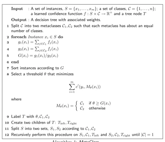
We now present a new algorithm that we call MetaClass (Algorithm 1). This algorithm is similar to that of Lachiche and Flach (2003) in that we reduce the multi-class problem to a series of two-class problems. However, we take what can be considered a top-down approach while the algorithm of Lachiche and Flach (2003) can be considered bottom-up. Moreover, MetaClass has a faster time complexity. The output of the algorithm is a decision tree with each internal node labeled by twometaclasses and a threshold value.
Each leaf node is labeled by one of the classes in the original problem. At the root, the set of all classes is divided into two metaclasses. The criterion for this split may be based on any statistical measure, but for simplicity, experiments were performed by splitting classes so that each metaclass would have roughly the same number of examples. For each metaclass, our algorithm defines confidence functionsg1(xi) andg2(xi)
for each instancexi, which are simply the sum of the confidences of the classes inC1 andC2, respectively.
The ratioG(xi) =g1(xi)/g2(xi) is used to find a thresholdθ. We findθby sorting the instances according
to G(xi) and choose a threshold that minimizes error. (This threshold will be the average of G(xi) and
G(xi+1) for some instancexi.) We recursively perform this procedure on the two metaclasses until there is
only a single class, at which point a leaf is formed.
The situation for nonuniform costs is slightly more complicated since it is not clear which class among those in metaclass an example is misclassified as. Recall that our cost functionc(y,yˆ) represents the cost of misclassifying an instance xof class y as class ˆy. However, in this case we need a cost function to quantify the cost of misclassifying an example into a set of classes. Formally, we need a functionc0 :C ×2C →R+. There are numerous natural extensions fromc to c0. For our experiments, c0 represents the average cost of misclassifying instances into metaclasses inC1 andC2. More formally, ifC0 ⊆ C, we definec0(y,C0) to be 0 if
y∈ C0 (that is,x’s true label class is in the metaclass) and
1 |C0|
X
j∈C0 c(y, j)
otherwise. TheMetaClassalgorithm is presented as Algorithm 1.
Input : A set of instances,S={x1, . . . , xm}; a set of classes, C={1, . . . , n};
a learned confidence functionf:S× C →R+ and a tree nodeT
Output: A decision tree with associated weights.
SplitCinto two metaclassesC1,C2 such that each metaclass has about an equal
1 number of classes. foreachInstancexi∈S do 2 g1(xi) =Pj∈C1fj(xi) 3 g2(xi) =Pj∈C2fj(xi) 4 G(xi) =g1(xi)/g2(xi) 5 end 6
Sort instances according toG
7
Select a thresholdθ that minimizes
8 m X i=1 c0(yi, Mθ(xi)) where Mθ(xi) = C1 ifθ≥G(xi) C2 otherwise LabelT withθ,C1,C2 9
Create two children ofT: Tleft, Tright
10
SplitSinto two sets,S1, S2 according toC1,C2
11
Recursively perform this procedure onS1,C1, TleftandS2,C2, Tright until|C|= 1
12
Algorithm 1: MetaClass
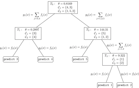
Figure 1 gives an example of a tree built by theMetaClass algorithm on the UCI (Blake & Merz, 2005) data set Nursery, a 5-class data set. At the root, the classes are divided into two metaclasses, each with about the same number of examples represented in their respective classes. In this case, the threshold θ= 0.8169 favors the sum of confidences in metaclassC1={4,3} as an optimal weight.
T0: θ= 0.8169 C1={4,3} C2={1,5,2} T1: θ= 0.2897 C1={3} C2={4} predict 3 g1(x) =f3(x) predict 4 g2(x) =f4(x) g1(x) = X j=3,4 fj(x) T2: θ= 144.31 C1={5} C2={1,2} predict 5 g1(x) =f5(x) T3: θ= 9.322 C1={1} C2={2} predict 1 g1(x) =f1(x) predict 2 g2(x) =f2(x) g2(x) = X j=1,2 fj(x) g2(x) = X j=1,2,5 fj(x)
Figure 1: Example run of MetaClasson Nursery, a 5-class problem.
Predictions for a new example xare made as follows. Starting at the root node, we traverse the tree towards a leaf. At each node T we compute the sum of confidences of x with respect to each associated metaclass. We traverse left or right down the tree depending on whether g1(x)/g2(x)≥θ. When a leaf is
reached, a final class prediction is made.
The number of nodes created byMetaClassis Θ(n), wherenis the number of classes. Since the split into two metaclasses ensures each has an equal number of classes,MetaClass results in a log (n)-depth tree. At each level, the most complex step is sorting at mostm instances according to the confidence ratio. Thus, the overall time complexity is bounded by O(mlogmlogn). This represents a significant speedup to the algorithm of Lachiche and Flach (2003), which requires Θ(nmlogm) time. Classification is also efficient. At each node we compute a sum over an exponentially shrinking number of classes. The overall number of operations is thus log (n)−1 X i=0 n 2i ,
which is linear in the number of classes: Θ(n). This matches the time complexity of Lachiche and Flach’s with respect to classification.
6
Experimental Results
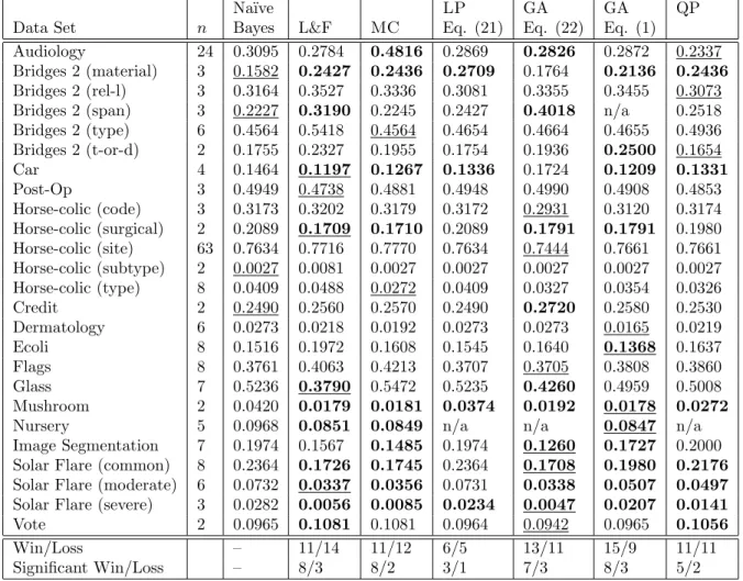
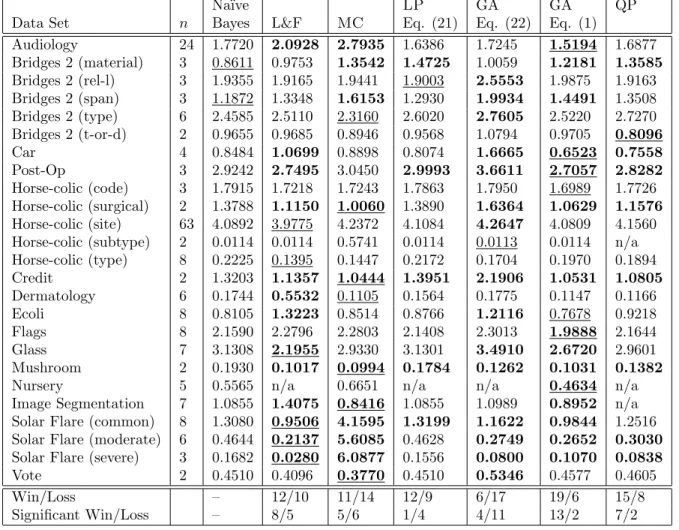
The following experiments were performed on 25 standard UCI data sets (Blake & Merz, 2005), using Weka’s na¨ıve Bayes (Witten et al., 2005) as the baseline classifier and Matlab’s optimization functions for reoptimization. We ran experiments evaluating improvements both in classification accuracy and under nonuniform cost. We used 10-fold cross validation for error rate experiments (Table 1). For the cost experiments of Table 2, 10-fold cross validations were performed on 10 different cost matrices for each data set. Costs were integer values between 1 and 10 assigned uniformly at random. Costs on the diagonal were set to zero. The average cost per test instance was reported for each experiment. Table 2 gives the average cost over all 100 experiments per data set, per algorithm.
Table 1: Error Rates. Na¨ıve Bayes is our baseline classifier. L&F is our implementation of Lachiche & Flach (2003). MC is MetaClass (Algorithm 1). LP, GA and QP are the Relaxed Integer Linear Programming, Genetic Algorithms and Quadratic Programming formulations optimizing their respective objective func-tions. Bold font denotes a significant difference to the baseline with at least 95% confidence according to the Student’stmethod. The overall best classifier among all algorithms is underlined.
Na¨ıve LP GA GA QP
Data Set n Bayes L&F MC Eq. (21) Eq. (22) Eq. (1)
Audiology 24 0.3095 0.2784 0.4816 0.2869 0.2826 0.2872 0.2337 Bridges 2 (material) 3 0.1582 0.2427 0.2436 0.2709 0.1764 0.2136 0.2436
Bridges 2 (rel-l) 3 0.3164 0.3527 0.3336 0.3081 0.3355 0.3455 0.3073 Bridges 2 (span) 3 0.2227 0.3190 0.2245 0.2427 0.4018 n/a 0.2518 Bridges 2 (type) 6 0.4564 0.5418 0.4564 0.4654 0.4664 0.4655 0.4936 Bridges 2 (t-or-d) 2 0.1755 0.2327 0.1955 0.1754 0.1936 0.2500 0.1654 Car 4 0.1464 0.1197 0.1267 0.1336 0.1724 0.1209 0.1331 Post-Op 3 0.4949 0.4738 0.4881 0.4948 0.4990 0.4908 0.4853 Horse-colic (code) 3 0.3173 0.3202 0.3179 0.3172 0.2931 0.3120 0.3174 Horse-colic (surgical) 2 0.2089 0.1709 0.1710 0.2089 0.1791 0.1791 0.1980 Horse-colic (site) 63 0.7634 0.7716 0.7770 0.7634 0.7444 0.7661 0.7661 Horse-colic (subtype) 2 0.0027 0.0081 0.0027 0.0027 0.0027 0.0027 0.0027 Horse-colic (type) 8 0.0409 0.0488 0.0272 0.0409 0.0327 0.0354 0.0326 Credit 2 0.2490 0.2560 0.2570 0.2490 0.2720 0.2580 0.2530 Dermatology 6 0.0273 0.0218 0.0192 0.0273 0.0273 0.0165 0.0219 Ecoli 8 0.1516 0.1972 0.1608 0.1545 0.1640 0.1368 0.1637 Flags 8 0.3761 0.4063 0.4213 0.3707 0.3705 0.3808 0.3860 Glass 7 0.5236 0.3790 0.5472 0.5235 0.4260 0.4959 0.5008 Mushroom 2 0.0420 0.0179 0.0181 0.0374 0.0192 0.0178 0.0272
Nursery 5 0.0968 0.0851 0.0849 n/a n/a 0.0847 n/a
Image Segmentation 7 0.1974 0.1567 0.1485 0.1974 0.1260 0.1727 0.2000 Solar Flare (common) 8 0.2364 0.1726 0.1745 0.2364 0.1708 0.1980 0.2176
Solar Flare (moderate) 6 0.0732 0.0337 0.0356 0.0731 0.0338 0.0507 0.0497
Solar Flare (severe) 3 0.0282 0.0056 0.0085 0.0234 0.0047 0.0207 0.0141
Vote 2 0.0965 0.1081 0.1081 0.0964 0.0942 0.0965 0.1056
Win/Loss – 11/14 11/12 6/5 13/11 15/9 11/11
Significant Win/Loss – 8/3 8/2 3/1 7/3 8/3 5/2
In both tables, for each data set, ndenotes the number of classes. The first column is the performance of our baseline classifier. For comparison, we have included results of our implementation for the algorithm of Lachiche and Flach (2003) on this baseline classifier. The results of the experiments on our heuristics can be found in the last five columns of each table. Here, MC is theMetaClass algorithm (Algorithm 1). LP is a linear programming algorithm (MOSEK ApS, 2005) on (21) with η = 10−6. The first GA is the
sum of linear fractional functions formulation (22) using a genetic algorithm. The second GA was a direct optimization performed on (1). Both GA implementations were from Abramson (2005). Parameters for both used the default Matlab settings with a population size of 20, a maximum of 200 generations and a crossover fraction of 0.8. The algorithm terminates if no change is observed in 100 continuous rounds. In addition, the mutation function of Abramson (2005) is guaranteed to only generate feasible solutions (in our case, all weights must be nonnegative). Upon termination, a direct pattern search is performed using the best solution from the GA. The final column is the quadratic program (QP) as in Section 5.1.3. Data for some entries were not available and are denoted “n/a” (data sets were too large for Matlab). For all columns,
bold entries indicate a significant difference to the baseline with at least a 95% confidence according to a Student’stmethod. The overall best classifier for each data set is underlined.
Table 2: Nonuniform Costs. Na¨ıve Bayes is our baseline classifier. L&F is our implementation of Lachiche & Flach (2003). MC is the MetaClass (Algorithm 1). LP, GA and QP are the Relaxed Integer Linear Programming, Genetic Algorithms and Quadratic Programming formulations optimizing their respective objective functions. Bold font denotes a significant difference to the baseline with at least 95% confidence according to the Student’st method. The overall best classifier among all algorithms is underlined.
Na¨ıve LP GA GA QP
Data Set n Bayes L&F MC Eq. (21) Eq. (22) Eq. (1)
Audiology 24 1.7720 2.0928 2.7935 1.6386 1.7245 1.5194 1.6877 Bridges 2 (material) 3 0.8611 0.9753 1.3542 1.4725 1.0059 1.2181 1.3585 Bridges 2 (rel-l) 3 1.9355 1.9165 1.9441 1.9003 2.5553 1.9875 1.9163 Bridges 2 (span) 3 1.1872 1.3348 1.6153 1.2930 1.9934 1.4491 1.3508 Bridges 2 (type) 6 2.4585 2.5110 2.3160 2.6020 2.7605 2.5220 2.7270 Bridges 2 (t-or-d) 2 0.9655 0.9685 0.8946 0.9568 1.0794 0.9705 0.8096 Car 4 0.8484 1.0699 0.8898 0.8074 1.6665 0.6523 0.7558 Post-Op 3 2.9242 2.7495 3.0450 2.9993 3.6611 2.7057 2.8282 Horse-colic (code) 3 1.7915 1.7218 1.7243 1.7863 1.7950 1.6989 1.7726 Horse-colic (surgical) 2 1.3788 1.1150 1.0060 1.3890 1.6364 1.0629 1.1576 Horse-colic (site) 63 4.0892 3.9775 4.2372 4.1084 4.2647 4.0809 4.1560 Horse-colic (subtype) 2 0.0114 0.0114 0.5741 0.0114 0.0113 0.0114 n/a Horse-colic (type) 8 0.2225 0.1395 0.1447 0.2172 0.1704 0.1970 0.1894 Credit 2 1.3203 1.1357 1.0444 1.3951 2.1906 1.0531 1.0805 Dermatology 6 0.1744 0.5532 0.1105 0.1564 0.1775 0.1147 0.1166 Ecoli 8 0.8105 1.3223 0.8514 0.8766 1.2116 0.7678 0.9218 Flags 8 2.1590 2.2796 2.2803 2.1408 2.3013 1.9888 2.1644 Glass 7 3.1308 2.1955 2.9330 3.1301 3.4910 2.6720 2.9601 Mushroom 2 0.1930 0.1017 0.0994 0.1784 0.1262 0.1031 0.1382
Nursery 5 0.5565 n/a 0.6651 n/a n/a 0.4634 n/a
Image Segmentation 7 1.0855 1.4075 0.8416 1.0855 1.0989 0.8952 n/a Solar Flare (common) 8 1.3080 0.9506 4.1595 1.3199 1.1622 0.9844 1.2516 Solar Flare (moderate) 6 0.4644 0.2137 5.6085 0.4628 0.2749 0.2652 0.3030
Solar Flare (severe) 3 0.1682 0.0280 6.0877 0.1556 0.0800 0.1070 0.0838
Vote 2 0.4510 0.4096 0.3770 0.4510 0.5346 0.4577 0.4605
Win/Loss – 12/10 11/14 12/9 6/17 19/6 15/8
Significant Win/Loss – 8/5 5/6 1/4 4/11 13/2 7/2
We observe that no one technique consistently produced the best performance on the most data sets. For this reason, the most relevant measure among these heuristics is the ratio of significant wins to significant losses rather than merely total wins or losses.
As far as classification error is concerned, with the exception of the linear programming relaxation, all algorithms were competitive with no clear overall winner in terms of significant wins and significant losses. However, every algorithm successfully showed substantial improvement over the baseline classifier. This confirms that the techniques presented serve as good reclassification methods in practice.
However, when we consider nonuniform costs, Table 2 indicates that the quadratic programming for-mulation and the genetic algorithm optimization on (1) outperform all other methods. In some sense, this reflects the inherent combinatorial nature of the problem, giving evidence that the objective function surface is likely to be very rough with many local minimums (it is certainly discontinuous given the use of the argmax function). This also may explain why other methods did not perform as well. The GA is searching globally; in contrast all other methods (including Lachiche and Flach (2003)) search locally. Even the in-teger linear programming relaxation, which in general has a good track record, came up short. Intuitively, the quadratic programming formulation should also suffer for these reasons, but fares better due to the
advantages characteristic of margin maximization techniques.
7
Conclusions and Future Work
Reoptimizing an already-learned classifier f is an important problem in machine learning, particularly in applications where the cost model or class distribution of a learning problem deviates from the conditions under which a classifier f was trained. We answered the open problem concerning the hardness of this reoptimization problem, and presented an algorithm that produces an optimal solution in polynomial time when the number of classes is constant. We also presented multiple algorithms for the multi-class version of this problem and empirically showed their competitiveness. Direct optimization by a genetic algorithm and quadratic programming were particularly effective under nonuniform cost models.
Acknowledgments
The authors would like to thank Nicolas Lachiche for helpful correspondence. We also thank anonymous reviewers for helpful suggestions and feedback. This work was supported in part by NSF grants CCR-0325463, CCR-0092761 and CCF-0430991.
References
Abramson, M. A. (2005). Genetic algorithm and direct search toolbox. http://www.mathworks.com/. Blake, C., & Merz, C. (2005). UCI repository of machine learning databases.
http://www.ics.uci.edu/ mlearn/MLRepository.html.
Boyd, S., & Vandenberghe, L. (2004). Convex optimization. Cambridge University Press.
Ferri, C., Hern´andez-Orallo, J., & Salido, M. (2003). Volume under the ROC surface for multi-class problems.
European Conference on Artificial Intelligence(pp. 108–120).
Fieldsend, J., & Everson, R. (2005). Formulation and comparison of multi-class ROC surfaces. Proceedings of the ICML Workshop on ROC Analysis in Machine Learning(pp. 41–48).
Hand, D., & Till, R. (2001). A simple generalisation of the area under the ROC curve for multiple class classification problems. Machine Learning,45, 171–186.
Kohli, R., Krishnamurti, R., & Mirchandani, P. (1994). The minimum satisfiability problem. SIAM Journal of Discrete Mathematics,7, 275–283.
Lachiche, N., & Flach, P. (1999). 1BC: A first-order bayesian classifier. Proceedings of the 9th International Workshop on Inductive Logic Programming(pp. 92–103).
Lachiche, N., & Flach, P. (2003). Improving accuracy and cost of two-class and multi-class probabilistic classifiers using ROC curves. Proceedings of the 20th International Conference on Machine Learning(pp. 416–423).
Matsui, T. (1996). NP-hardness of linear multiplicative programming and related problems. Journal of Global Optimization,9, 113–119.
MOSEK ApS (2005). The MOSEK optimization tools version 3.2. http://www.mosek.com/. Mossman, D. (1999). Three-way ROCs. Medical Decision Making, 78–89.
O’Brien, D. B., & Gray, R. M. (2005). Improving classification performance by exploring the role of cost matrices in partitioning the estimated class probability space.Proceedings of the ICML Workshop on ROC Analysis in Machine Learning(pp. 79–86).
Rockafellar, R. (1970). Convex analysis (2nd ed.). Princeton University Press. Sch¨olkopf, B., & Smola, A. (2002). Learning with kernels (2nd ed.). MIT Press.
Srinivasan, A. (1999). Note on the location of optimal classifiers in n-dimensional ROC space (Technical Report PRG-TR-2-99). Oxford University Computing Laboratory, Oxford.
Stoer, I. J., & Witzgall, C. (1996). Convexity and optimization in finite dimensions. Springer-Verlag. Witten, I. H., et al. (2005). Weka machine learning toolbox. www.cs.waikato.ac.nz/ml/weka/.