Umair Akhtar Hasan Khan
Prostate Cancer Detection
Using Deep Learning
Faculty of Information Technology
and Communication Sciences
M.Sc. Thesis
March 2019
ABSTRACT
Umair Akhtar Hasan Khan : Prostate Cancer Detection using Deep Learning M.Sc. Thesis Tampere University Degree Programme in Computer Science April 2019 Supervisors: Martti Juhola and Kati IltanenCancer detection is one of the principal topics of research in medical science. May it be breast, lung, brain or prostate cancer, advances are being made to improve detection precision and time. Research is being carried out on broad range of procedures at different stages of cancer to understand it better. Prostate cancer, in particular, has seen some novel approaches of detection using both magnetic resonance imaging (MRI) and histopathology data. The approaches include detection using deep neural networks, deep convolutional neural networks in particular because of their human level precision in image recognition task.
In this thesis, we analysed a dataset containing multiparametric magnetic resonance imaging (mpMRI) prostate scans. The objective of the research was Gleason grade group classification, through mpMRI scans, which has not been attempted before on a small dataset. We first trained several conventional machine learning algorithms on handcrafted features from the dataset to predict the Gleason grade group of the cases. After that the dataset was augmented using two different augmentation techniques for further experimentation with deep convolutional neural networks. Convolutional neural network of varying depth were used to understand the effects of network depth on classification accuracy. Furthermore, we made an attempt to shed light on the pitfalls of using small dataset for solving problems of such nature.
Keywords: Deep Neural Networks, multiparametric Magnetic Resonance Imaging (mpMRI), Convolutional Neural Networks
The originality of this thesis has been checked using the Turnitin Originality Check service.
ACKNOWLEDGEMENT
I would like to take the opportunity to thank Timo Heikkinen (CEO, Top Data Science) for hiring me for this research project and providing me the opportunity to work on cutting edge technologies. I’d like to thank my supervisors Martti Juhola (Professor, Tampere University) and Kati Iltanen (Dean, Faculty of Natural Sciences, Tampere University ) for their support and guidance. I feel very fortunate to have them as my supervisors, their positive feedback and constructive criticism always pushed me to refine my work to the highest level.
Last but not the least, I am grateful to Oguzhan Gencoglu (Head of Data Science, Top Data Science) for all the guidance and knowledge he shared with me, not only did he guide me throughout the course of this research project but also inspired me to deliver quality work. I am impressed with his attention to detail and dedication to the project. Working with him helped me instill the same traits in myself.
Once again, I’d like to express my gratitude to all the people mentioned above, without them I would not have been able to execute this project.
CONTENTS
1. INTRODUCTION 8 1.1 Prostate Cancer 8 1.2 Machine Learning 9 1.3 Artificial Neural Networks 11 1.4 Deep Learning and Deep Neural Networks 12 1.5 Thesis Problem Statement 13 1.6 Aim and Objective 13 2. LITERATURE REVIEW 14 2.1 Computeraided Diagnosis (CAD) for Prostate Cancer 14 2.1.1 Conventional Machine Learning based CAD 14 2.1.2 Deep Learning based CAD 17 2.2 State of the Deep Neural Network Architectures 22 2.2.1 Inception V1 23 2.2.3 InceptionV3 25 2.2.4 Xception 26 2.2.5 Deep Residual Learning for Image Recognition 28 3. DATASET AND FRAMEWORKS 31 3.1 Dataset 31 3.1.1 Exploratory Analysis 32 3.2 Technology and Frameworks 35 3.3 Data Wrangling 35 3.3.1 Image Augmentation 35 3.3.1.1 Standard Augmentation 35 3.3.1.2 Extended Augmentation 36 3.4 Evaluation Metrics 36 3.4.1 Accuracy Score 36 3.4.2 Cohen’s Kappa 37 4. PROPOSED METHODS 38 4.1 Feature engineering 38 4.2 Conventional Machine Learning 39 4.2.1 Bernoulli Naive Bayesian 40 4.2.2 Passive Aggressive 40 4.2.3 KNearest Neighbors 43 4.2.4 Random Forest 44 4.2.5 Support Vector 44 4.2.6 Logistic Regression 45 4.2.7 Linear and Quadratic Discriminant Analysis 46
4.3 Convolutional Neural Networks 47 4.3.1 Vanilla Model and variations 48 4.3.2 Xmasnet Model 49 4.4 Pretrained StateoftheArt Deep Networks 50 5. EXPERIMENTS AND RESULTS 52 5.1 Conventional Classifiers with Image features 52 5.1.1 Single Slice ROI 5Fold Cross Validation 52 5.1.2 MultiSlice ROI 5Fold Cross Validation 55 5.2 Partially Trained InceptionV3 57 5.3 Vanilla Models 58 5.4 Xmasnet Model 60 5.5 MultiChannel Experiments 61 5.5.1 Slices to Channel 61 5.5.2 Modality to Channel 62 5.6 Feature Extraction with Shallow Network and training with Conventional Machine Learning Algorithms 62 6. CONCLUSION 63 7. REFERENCES 64
LIST OF FIGURES
Figure 1: Classification using support vector machine (SVM). Figure 2: Visualisation of a basic neural network. Figure 3: Visualisation of GoogleNet [ Szegedy et al., 2016 ]. Figure 4: Suggested workflow for the proposed CAD system [ Litjens et al., 2015 ]. Figure 5: Generating a threechannel RGB image from three mpMRIs [ Tsehay et al., 2017 ]. Figure 6: a. Examples of the four types of input images for XmasNet. b. Illustration of data augmentation through 3D slicing. c. Illustration of data augmentation through inplane rotation. The dashed box is a 32×32 region of interest (ROI) centered at the lesion. Figure 7: Comparison of real and synthetic ROI patches [ Kitchen & Seah, 2017 ]. Figure 8: An inception module with dimensionality reduction. Figure 9: Inception modules [ Szegedy et al., 2016 ]. Figure 10: Xception architecture [ Chollet, 2016 ]. Figure 11: Residual Learning: a building block [ He et al., 2015 ]. Figure 12: 34Layer Resnet [ He et al., 2015 ]. Figure 13: Gleason grade groups [ “How is Prostate Cancer Diagnosed?”, 2018 ].Figure 14: T2 weighted scan (sagittal and transaxial plane), apparent diffusion coefficient and bvalue scan with ROI highlighted with a red bounding box.
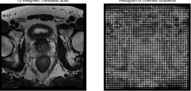
Figure 15: Bar chart showing zone information distribution, AS: anterior fibromuscular stroma, PZ: peripheral zone, TZ: transition zone. Figure 16: Pie chart showing Gleason grade groups distribution. Figure 17: Image augmentation techniques. Figure 18a: Histogram of oriented gradients calculated from T2weighted transaxial scan. Figure 18b: Local binary pattern calculated from T2weighted transaxial scan. Figure 19: Vanilla model network diagram.
Figure 20: The architecture of the XmasNet. Conv: convolutional layer; BN: batch normalization layer; ReLU: rectified linear unit; Pooling: max pooling layer; FC: fully connected layer. Figure 21a: Original dataset dimensionality reduction (T2weighted transaxial scan). Figure 21b: Augmented dataset dimensionality reduction (T2weighted transaxial scan). Figure 22: Kappa score vs. Accuracy scatter plot for T2weighted transaxial scan. Figure 23: Single vs. Multislice bar chart for T2weighted transaxial scan. Figure 24: Partially trained InceptionV3, fold wise accuracy.
Figure 25: Xmasnet model vs. InceptionV3 accuracy bar chart for T2weighted sagittal plane
LIST OF TABLES
Table 1: Camelyon 16 data distribution
Table 2: GoogleNet incarnation of Inception architecture [ Szegedy et al., 2015 ] Table 3: InceptionV3 model [ Szegedy et al., 2016 ]
Table 4: Conventional classifiers accuracy and Kappa score for HOG descriptors computed on single slice ROI
Table 5: Conventional classifiers accuracy and Kappa score for LBP descriptors computed on single slice ROI
Table 6: Conventional classifiers accuracy and Kappa score for LBP+HOG descriptors computed on single slice ROI
Table 7: Conventional classifiers accuracy and Kappa score for HOG descriptors computed on multislice ROI
Table 8: Conventional classifiers accuracy and Kappa score for LBP descriptors computed on multislice ROI
Table 9: Conventional classifiers accuracy and Kappa score for LBP+HOG descriptors computed on multi slice ROI Table 10: InceptionV3 140x140 ROI from T2weighted sagittal plane scan 5fold CV Table 11: Vanilla model configuration Table 12: Vanilla model accuracy and Kappa score for T2weighted sagittal plane scan Table 13: Xmasnet Model accuracy and Kappa score for T2Weighted Sagittal plane scan Table 14: Accuracy and Kappa score for slices to channel experiment Table 15: Accuracy and Kappa score for modality to channel experiment Table 16: Xgboost and SVM results trained on shallow network bottleneck features
LIST OF ABBREVIATIONS AND ACRONYMS
ADC Apparent Diffusion Coefficient AUC Area Under the Curve BVAL BValue CAD Computer Aided Diagnosis CNN Convolutional Neural Network DCE Dynamic Contrast Enhanced DL Deep Learning DWI DiffusionWeighted Imaging GGG Gleason Grade Group HOG Histogram of Oriented Gradients ILSVRC Imagenet Large Scale Visual Recognition challenge KS Kappa score LBE Lesionbased Evaluation LBP Local Binary Pattern LDA Linear Discriminant Analysis LR Logistic Regression mpMRI Multiparametric Magnetic Resonance Image PCA Principal Component Analysis PIRADS Prostate Imaging Reporting and Data System PssAgg Passive Aggressive Classifier QDA Quadratic Discriminant Analysis ReLU Rectified Linear Unit RNN Recurrent Neural Network RCNN Regional Convolutional Network ROC Receiver Operating Characteristic ROI Region of Interest SBE Slicebased Evaluation SVC Support Vector Classifier SVM Support Vector Machine TF Tensorflow TSE_SAG T2Weighted Sagittal TSE_TRA T2Weighted Transaxial TSNE tDistributed Stochastic Neighbor Embedding WSI WholeSlide Image VGG Visual Geometry Group1. INTRODUCTION
Prostate cancer is the most common cancer in men after skin cancer in America. One man in nine will develop clinically significant prostate cancer and one man in forty one will die of it. A combination of invasive and noninvasive techniques, such as Transrectal ultrasound guided (TRUS) biopsy and Multiparametric Magnetic Resonance Imaging (mpMRI) respectively, have enabled us to accurately diagnose the aggressiveness of prostate cancer. The type and course of treatment is then decided, based on the stage of the cancer, it could be any of the following surgery, radiation therapy, cryotherapy, hormone therapy or chemotherapy. [ “Key Statistics for Prostate Cancer”, 2018 ].
Having said that, during the last two decades, a separate vertical, although not directly related to medical science, has been analysing medical data and making strides, especially in diagnosis. Computer scientists, with the help of image processing and machine learning algorithms, have been fine tuning their systems to diagnose different types of cancerous nodules, cysts and tumors. They call it Computeraided Diagnosis (CaD). Some of the recent endeavours have surpassed human accuracy. These CaD techniques are driven by Deep Neural Networks which are discussed in the following chapters. At this stage the idea is to not completely eliminate human involvement from the diagnosis process, rather to introduce a hybrid system consisting of CaD as well as human diagnosis where both systems are complementary to each other, resulting in significant improvement in cancer detection.
1.1 Prostate Cancer
The prostate is a gland responsible for making most of the sperm carrying semen in the male reproductive system. It sits between the bladder and the upper part of urethra which carries the urine from the bladder. [ “The Basics of Prostate Cancer”, 2018 ].
Prostate cancer is quite common in Finland with more that 4700 cases of prostate cancer are recorded each year in Finland [“ Docrates is the first oncology center in Finland to offer new radiation therapy for metastatic prostate cancer ”, 2018]. Cancer at an early stage is curable, a vast majority patients undergo treatments which completely cure them. Therefore, early diagnosis of cancer is pivotal in curing cancer. However, prostate cancer at an advanced stage can not be completely cured and requires perpetual treatment. In case of American men about 85% of cases diagnosed with prostate cancer are in early stage of the disease, where it has not spread much [ “The Basics of Prostate Cancer”, 2018 ].
If the cancer spreads beyond the prostate for example to bones, lungs or lymph nodes, then it is no more curable, but advancement in medical science has enabled us to keep it under
control and the life span of the patient can be extended to several years. In some cases it has been observed that patients with advanced prostate cancer lived for many years and their cause of death was entirely different from prostate cancer.
Prostate cancer is generally found in older men. Over 80% of men diagnosed with prostate cancer are over 65 years of age and less than 1% are under 50. Susceptibility to prostate cancer increases if a person has family history of it. There is not yet an established research on the exact cause of cancer; however, prostate cancer is linked with certain types of diet which include overconsumption of fats and red meat. Substance produced as a byproduct of meat cooked on high temperature is dangerous for a prostate. The rate of prostate cancer varies in countries, based on their food consumption. It is common in countries with high consumption of dairy products and meat as compared to countries with vegetable and rice based diet.
Hormones are another factor. Testosterone increases with higher consumption of fats which works as a catalyst in the growth of prostate cancer. Lack of exercise also makes prostate cancer more likely. A few occupational hazards have also been found to be contributing factors to prostate cancer. For example, some jobs in rubber and battery manufacturing require workers to be exposed to metal cadmium, which make them prone to getting prostate cancer. Drugs such as aspirin, finasteride (Proscar) and dutasteride (Avodart) have proven to reduce the risk of developing prostate cancer. Similarly, regular consumption of some vegetables such as broccoli, cauliflower, and cabbage have also been a deterrent to prostate cancer [ “The Basics of Prostate Cancer”, 2018 ].
1.2 Machine Learning
The overlap of the fields of computer science and statistical methods gave birth to the field of machine learning. Machine learning enables computer programs to progressively learn which does not necessitate any explicit programming assistance. Arthur Samuel came up with the term machine learning. [ Samuel, 1988 ]. The field of machine learning evolved as the amalgamation of pattern recognition and computational learning theory in artificial intelligence [ “ Machine learning | artificial intelligence ”, 2018 ]. The aim of machine learning is the construction of such algorithms that can learn from data and make predictions on unseen data, the outcome of such algorithms are not contingent on any strict programmatic logic. Primarily there are two types of learning, supervised and unsupervised. [Mohri et al., 2012; Trucker, 2004]
Supervised learning: In supervised learning learning the data is fed to the program along with the corresponding labels, the theme is to learn a function that maps the data to its label. However, there are special cases of
● SemiSupervised learning: In semisupervised learning the training data has incomplete labels, in most cases the input data has missing labels.
● Reinforcement learning: In reinforcement learning the data is fed to the algorithm from a dynamic environment in form of rewards and punishments. It could be playing a first person shooting game against multiple opponents or flying a plane in a simulated environment.
Unsupervised learning: In unsupervised learning, no labels are provided to the learning algorithm, the algorithm relies on hidden patterns and structure in the data for learning. An auxiliary purpose of unsupervised learning could be to find out the intrinsic patterns or learn features of the data.
Machine learning can also be categorized on the basis of the type of desired output of a machine learning system.
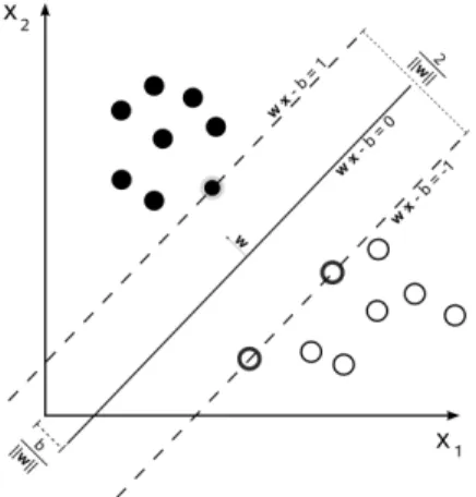
Classification: In classification the input data is divided into two or more classes, the learning algorithm learns a mapping function during training and assigns one or more of these classes to an unseen data point either during testing or in an actual use case. This is typically done is a supervised way. [Alpaydin, 2010]. Figure 1 visually illustrates support vector machine (SVM) [ Cortes & Vapnik, 1995 ], a classifier that separates its input space into two regions using a linear boundary.
Regression: Unlike classification the output variable of regression is continuous. Regression too is usually done in a supervised way [Freedman, 2009].
Clustering: Clustering is an unsupervised task in which the input is divided into k number of groups using different clustering algorithms [Bailey, 1994].
Density Estimation: Density estimation finds the distribution of inputs in some space [“2.8. Density Estimation”, 2018].
Dimensionality Reduction: It is a process of transforming high dimensional data to lower dimension [Roweis et al., 2000]. One of the applications of dimensionality reduction is visualisation of data in either two of three dimensional space.
Figure 1: Classification using support vector machine (SVM).
In the present era it is difficult to find a field which is not disrupted by machine learning or to say the least affected by it. May it be stock predictions, virtual personal assistance, video
surveillance, social media, customer support, spam filtering, weather prediction or online fraud detection; machine learning has affected each one of them. Among these, the field which has seen very serious efforts and interest is medical science. Machine learning is now solving as complicated problems as cancer/tumor detection which is a nontrivial problem by any definition. Computer aided diagnosis solutions for cancer detection are at the crossroads of computer vision and machine learning. Over time these solutions have gone through an evolutionary process which tremendously improved their efficiency and effectiveness.
1.3
Artificial Neural Networks
The idea of artificial neural networks is roughly based on the working of a human brain, it is inspired by the biological neural network. An artificial neural network (ANN) based system learns progressively without task specific programming [ “Artificial Neural Networks as Models of Neural Information Processing”, 2018 ]. For instance, an ANN capable of image recognition learns to identify objects that are manually labelled, e.g. it can tell apart images that contain a car from images that do not contain a car. These networks can learn without any prior information about the features of a car.
An artificial neural network consists of connected layers of nodes called neurons, much similar to neurons in an animal brain. Connections between neurons simulate the function of synapse by transmitting information from one neuron to another. After receiving a signal, an artificial neuron can process it based on a certain function and can pass it to other artificial neurons. ANNs are implemented in a way that a real number passes as a signal through connections between artificial neurons. The output of each artificial neuron is calculated by a nonlinear function of the sum of its inputs. Part of the nonlinear function is a weight which modulates as the network learns during the training process. Weight is pivotal in determining the strength of the signal over a connection. Artificial neural network generally consists of layers stacked with artificial neurons, layers may differ from each other with respect to how they transform the inputs. Usually, signals iterate from first layer to the last, several times optimally adjusting the weights of artificial neurons in each iteration. [ “Artificial Neural Networks as Models of Neural Information Processing”, 2018 ].
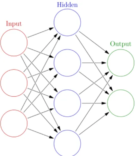
Originally the idea of ANN was inspired by human brain; however, the focus deviated from biological path over time in order to solve specific problems. Presently, ANNs are being used in a wide range of fields such as natural language processing, computer vision, speech recognition, video games, and medical science. Figure 2 is a visual representation of a basic artificial neural network.
Figure 2: Visualisation of a basic neural network.
1.4
Deep Learning and Deep Neural Networks
Deep learning is a subdiscipline of machine learning that is philosophically based on indepth learning from data, comprising of several layers of representations. The learning takes place in a hierarchical fashion, where learning at higher layers is extracted from learnings of lower layers. This process of concept learning in the domain of deep learning is called feature learning or representation learning. Input (for instance image data) can be represented in different ways (like a matrix containing pixel information), but some representations are more efficient than other in terms of learning features from data, and rapid advancements are being made in the area to make representation more efficient. [ Deng & Yu, 2014 ]
Generally, artificial neural networks are the key component of deep learning models. However, certain types can comprise of syntactic formula or latent (unobserved) variables structured layerwise in deep generative models, for instance the nodes in Deep Boltzmann Machines.
Learning in deep networks varies from layer to layer, in terms of level of abstraction and transformation of input data. In case of image processing, the data could be a 3 dimensional array of pixels: the first representational layer captures the understanding of edges, the second representational layer may capture the sequence or arrangement of edges, the third representational layer may capture features of a car such as formation of tyres, windscreen, headlights, wipers and the fourth layer may discern the presence of a car in the image. Deep learning is capable of appropriately allocating the feature learning to specific layers and that too is learned. This, however, does not eliminate the need of manual configuration of a network, for instance, the number and size of layers have big impact on the performance and output of a deep learning model. [ Bengio et al., 2012 ; LeCun et al., 2015 ]
Deep learning can be employed for both supervised and unsupervised learning. In supervised learning it eliminates the process of feature engineering by learning terse transitional representations similar to principal components. Unsupervised learning is a good use case for deep learning because of the abundance of unlabeled data, it can be done using deep belief networks [ Hinton, 2009 ] and neural history compressors [ Schmidhuber, 2015 ]. Figure 3 is a visual representation of a fully connected deep neural network.
Figure 3: Visualisation of a fully connected deep neural network with n hidden layers.
1.5 Thesis Problem Statement
In this thesis research, the analysis of the mpMRI scans and metadata lead to the formulation of the problem statement. The idea was to use the mpMRI scans and train a machine learning model which can later be employed to detect the prostate cancer aggressiveness based on Gleason grade group of unseen cases. The 5 different Gleason grade groups make it a multiclass classification problem. Multiclass classification is a more complex problem than binary classification of clinical significance of cancer given the class imbalance and small size of the dataset. Moreover, an auxiliary challenge was the small size of the dataset, which was dealt with by engineering suitable techniques to augment the data.
1.6 Aim and Objective
The aim of this research was to use a small dataset and test how effectively deep learning can be applied on it to get meaningful results. Furthermore, a smaller dataset compelled us to experiment with different augmentation techniques as well.
2. LITERATURE REVIEW
A considerable amount of work has been done, both, in the domain of prostate cancer and the technology (computer vision and artificial intelligence). Research on cancer detection, in general, has gained a lot of traction in recent past. Research is being conducted using different types of artifacts such as mpMRI scans, CT scans and histopathological slides to understand and detect cancer better. There has been an increase in online competitions for cancer detection and its clinical significance. These competitions include breast, prostate, lung and brain cancer detection. But medical science is a domain, riddled with scarcity of data and it is one of the biggest challenges to overcome before we even begin to think about ANN model building and classification. This section elucidates the cutting edge research being done in the CAD area for cancer detection, prostate cancer detection in particular. It also explains the inner workings of the most advanced image recognition artificial neural networks being used in ImageNet Large Scale Visual Recognition Competition [ Russakovsky et al., 2014 ].
2.1 Computeraided Diagnosis (CAD) for Prostate Cancer
Computeraided diagnosis (CAD) are systems that help doctors and physicians interpret and understand medical images better. Images captured through Xrays, MRI and microscopes contain a tremendous amount of minute details which are supposed to be analysed and interpreted by radiologist, histopathologists and other medical professionals in a relatively short amount of time. Typically the idea behind CAD systems is to accentuate anomalous information in the scans in order to make it discernable for medical professionals to aid their decision.
Moore's law (roughly) states that the processing power doubles every 18 months [ Moore, 2006 ], the paper was written in 1965 and the law still holds. With ever so fast processors and advancement in the hardware field, another field has catched up and progressed quite a lot in recent years, that is machine learning. In today’s age, every field is employing machine learning driven solutions to bring about performance improvements, which were never witnessed before. CAD systems also happen to be one of the areas where machine learning has achieved human level results and there are instances where machine learning driven solutions proved to have done better than humans.
2.1.1 Conventional Machine Learning based CAD
As mentioned earlier that one of the biggest challenges in the field of medical science, when it comes to machine learning driven systems, is the dearth of data. Since a typical machine
learning system requires a large and comprehensive dataset in order to have good generalising power; therefore, researchers came up with a workaround to tackle this challenge. They started using synthetic data to train machine learning models.
A solution proposed by [ Fehr et al., 2015 ] solved the data size problem using Synthetic Minority Oversampling Technique SMOTE [ Chawla et al., 2002 ] and Gibbs sampling [ Geman & Geman, 1984 ]. The motivation behind the solution was to improve the efficacy of the noninvasive MRI scan in detecting initial stage benign cancer without necessarily subjecting patients to invasive procedures such as biopsy. The fundamental idea of the research was to perform classification based on Gleason scores, distinguishing Gleason scores 6 (3 + 3) from scores above or equal to 7 and Gleason score 7 (3 + 4) from 7 (4 + 3). The research used two different image modalities T2weighted MR images and apparent diffusion coefficient ADC to calculate image texture features.
T2weighted and ADC MR images were preprocessed and two sets of texture based features were engineered from these images. The first set of features included moments of the intensity volume histogram (mean, SD, skewness, and kurtosis) computed from the region of interest. The second set of features consisted of Haralick features [ Haralick et al., 1973 ] was computed using the gray level cooccurrence matrix (GLCM) with 128 bins and consisted of energy, entropy, correlation, homogeneity, and contrast. Both sets of features were then used to train SVM [ Cortes & Vapnik, 1995 ], SVM with (ttest and RFE) and Adaboost models. It was observed that even with a high imbalance in the classes, data augmentation helped obtaining high specificity and sensitivity. Finally, SVM combined with recursive feature elimination yielded best classification accuracy, distinguishing Gleason score 6 (3 + 3) from scores above or equal to 7 with 93% accuracy and Gleason score 7 (3 + 4) from 7 (4 + 3) with 92% accuracy.
Another solution took a similar approach of using conventional machine learning algorithms such as SVM and decision trees with image features based on texture, morphological scale invariant feature transform (SIFT) [ Cortes & Vapnik, 1995; Lowe, 2004 ], and elliptic Fourier descriptors (EFDs) [ Soldea et al., 2010 ] to detect clinically significant prostate cancer [ Hussain et al., 2018 ]. The dataset used in this study is publicly available by Harvard University (National Center for Image Guided Therapy Department of Radiology, Brigham and Women's Hospital, Harvard Medical School). The database is publicly available for research purposes. The study used a total of 682 MRI scans from 20 patients consisting of 482 images from prostate subjects and 200 images from brachytherapy subjects for the purpose of feature extraction and to use those features to detect cancer.
Models were trained using single as well as combination of feature sets for the task of classification. Jackknife [ Efron, 1979 ] and kfold were employed as cross validation techniques to ensure performance evaluation validity. Receiver Operating Characteristic (ROC), specificity, sensitivity, positive predictive value (PPV), negative predictive value
(NPV), false positive rate (FPR) were used to evaluate the strength of model. For single feature sets, SVM with Gaussian kernel gave the highest accuracy of 93.34% with an AUC score of 0.999. Whereas, for a combination of different feature sets SVM Gaussian kernel with texture morphological features gave the highest accuracy of 99.71% and AUC of 1.00.
A study conducted in 2015 took a rather unconventional approach of combining a CAD system and prostate imaging reporting and data system (PIRADS) score [ “Global PIRADS Standardization of Prostate MRI”, 2018 ] to detect prostate cancer [ Litjens et al., 2015 ]. The approach used in the study is a three step approach. In the first step, the system extracted quantitative voxel features from mpMRI scans, following PIRADS guidelines in order to capture characteristics described by the PIRADS guidelines. These voxel features were used as input to train a random forest classifier to determine a continuous likelihood score for each voxel for cancer identification, resulting in a likelihood image. The second step predicted cancer likelihood per lesion using a random forest classifier, trained by using a combination of the symmetry, local contrast and statistical features. Probability based segmentation of the prostate zones enabled the system to consider a lesion's zonal location. The third and final step drew a contrast between CAD, PIRADS and their combination using logistic regression and evaluated them based on ROC AUC score. Figure 4 describes the workflow of a CAD system.
Figure 4: Suggested workflow for the proposed CAD system [ Litjens et al., 2015 ].
The final analysis of the study included a total of 107 patients with 141 lesions. The ROC AUC score of the combination (CAD and PIRADS) was significantly higher than the PIRADS only score of the radiologist. In case of benign vs cancer, the combination score was 0.88, whereas radiologist score was 0.81 and the pvalue was 0.013. In case of indolent vs. aggressive, the scores were 0.88 and 0.78 with pvalue < 0.01 for combination and radiologist respectively. The actual cancer grade and combination score had a higher correlation (0.69, pvalue=0.0014) as compared to the individual CAD system or radiologist alone (0.54 and 0.58 respectively). It was concluded that the solution based on the combination of CAD and PIRADS had the potential to improve cancer detection accuracy.
2.1.2 Deep Learning based CAD
Ever since deep learning started making strides in image recognition and outclassed other conventional techniques, it has become synonymous with a panacea. Researchers with highly efficient GPU powered compute resources and advanced deep learning libraries such as TensorFlow at their disposal, are using these latest resources to come up with CAD systems to solve primitive problems. Deep neural networks are being used not only to detect prostate cancer but also segmentation of prostate in threedimensional space. A special kind of neural network called Generative Adversarial Network (GAN) [ Goodfellow et al., 2014 ] is found to be very effective in solving insufficient data problem. It generates very similar synthetic data points based on features learned from the actual dataset.
A study in 2017 drew a comparison between traditional machine learning CAD and deep learning based CAD [ Tsehay et al., 2017 ]. The approach used in this study was based on an edge detector network, which processes input images to generate their respective probability maps. The performance of this deep learning based CAD was evaluated using receiver operating characteristic (ROC) curve and freeresponse ROC (FROC). Then the performance of deep learning based CAD was compared with an already existing CAD which used SVM with handwrought features, such as local binary pattern (LBP) [ He, et al., 1990 ] extracted from the same dataset. The study included data of 52 patients in three different modalities, namely, T2W, ADC, and B2000 MR images. Since these modalities captured information about the same instance of the organ stored in different ways; therefore, it provided room to employ a novel approach of superimposing these modalities to create a threechannel RGB image as shown in Figure 5. The enriched threechannel input allowed the network to exploit the contrast of the image to learn meaningful features. Furthermore, the contrast of the RGB image was enhanced using histogram equalisation.
Figure 5: Generating a threechannel RGB image from three mpMRIs [ Tsehay et al., 2017 ].
The performance of deep learning based CAD was compared with the SVM based CAD that used the handwrought features. DL based CAD had an 86% true positive rate and 20% false positive rate. Whereas, the SVM based CAD had 80% true positive rate and 20% false positive rate, which when projected on the FROC came out to be 94% and 85% detection rate at 10 false positives per patient. The results were conclusive enough to establish that DL based CAD had potential and further exploration could lead to even better results.
A study which emerged as a result of an online competition PROSTATEx challenge [ “PROSTATEx Grand Challenge”, 2018 ] used a novel deep learning architecture named XmasNet to detect clinical significance of prostate cancer [ Liu et al., 2017 ]. The deep learning architecture (XmasNet) comprised of several convolutional layers. The dataset comprised of 341 cases and there were 4 different multiparametric MRI modalities, namely, diffusion weighted images (DWI), apparent diffusion coefficient (ADC), Ktrans and T2Weighted images. A unique way of data augmentation based on 3D rotation and slicing was employed to incorporate the information of the lesion as shown in Figure 6 part c. The study used a similar approach of superimposing modalities used in the aforementioned study [ Tsehay et al., 2017 ] to create a threechannel RGB image as shown in Figure 6 part a. The training set comprised of 274 lesions and validation set had 43 lesions. Based on the superimposition technique, four different types of inputs were generated using DWI (D), ADC (A), Ktrans (K), and transverse T2WI (T) as the RGB channels: DAK, DAT, AKT, DKT (shown in the figure before). Separate deep learning models were trained for each input type. 207144 training samples were generated after augmentation using inplane rotation, random shearing and translation for every slice. Each sample was 32x32 region of interest (ROI), surrounding the lesion. Figure 6: a. Examples of the four types of input images for XmasNet. b. Illustration of data augmentation through 3D slicing. c. Illustration of data augmentation through inplane rotation. The dashed box is a 32×32 region of interest (ROI) centered at the lesion [ Liu et al., 2017 ].
87 handcrafted features were used to train 140 decision trees using a gradient boosting algorithm called Xgboost [Chen & Guestrin, 2016] . The features included mean, standard deviation and intensities of each lesion along with texture features such as energy and
contrast. Experiments on the validation set proved that XmasNet with a ROC AUC score of 0.95 with sensitivity of 0.89 and specificity of 0.89, outperformed the best XGBoost model with ROC AUC score of 0.89 with sensitivity of 0.87 and specificity of 0.77. On the training set XmasNet achieved a score of 0.83 to become the second best score in the competition.
As mentioned earlier, one of the biggest challenges in using medical science data, especially visual data in deep learning, is its insufficient size. Enormity of data is one of the essentials for most deep learning models. Researchers have been working on exploring new ways to synthetically augment the data. Data augmentation can profoundly impact the learning of deep neural networks. One such approach is called Generative Adversarial Networks (GAN) [ Goodfellow et al., 2014 ]. A study on the same ProstateX dataset uses Generative Adversarial Networks to generate synthetic data samples [ Kitchen & Seah, 2017 ]. Generative models can be used to generate new data that looks very similar to the real data. A generative model's ability to encompass the data distribution itself, as opposed to conditional probability of a certain label given the data, makes it suitable for the task of data augmentation, unlike a discriminative models:
P(X|Y) Discriminative Model P(X) Generative Model
where P(X) is the data distribution and P(Y|X) is the conditional distribution of target variable given the data distribution.
A generative adversarial network can be generalised by using an analogy of a game played between two players with distinct competing objectives. The two players are the generator G and a discriminator D. G is a content generator that tries to create realistic looking content. D is a judge that tries to classify the authenticity of a content as fake or original. The principal equilibrium strategy in this game is for G to draw from P(X) in which case D performs no better than random guessing, i.e. the best way for G to fool D is to create content that are indistinguishable from real content (according to D). Generative model do not really have a global loss function for performance gain, instead these models are trained to an equilibrium point where neither player can improve their performance given a small unilateral change to their strategy; where their strategy is represented by continuous neural network weights. A leapfrog gradient descent algorithm is used for training, where a gradient descent step is taken for G with D held constant, then D with G held constant. With some luck and under conditions, that are in general not well understood, this algorithm can move both players into a suitable equilibrium strategy. This method is particularly powerful if the discriminative models are large Deep Convolutional Neural Networks. If there are any recognizable statistical aberrations in the data generated by G, then D can catch out the generator by recognizing these aberrations. Unrealistic structures are thus suppressed when training has reached equilibrium — G produces highly realistic samples. [ Kitchen & Seah, 2017 ]. The
study uses the same logic to develop generator and discriminator architectures and train them to produce 200 synthetic samples. Samples of real and synthetic lesions are shown in Figure 7.
Figure 7: Comparison of real and synthetic ROI patches [ Kitchen & Seah, 2017 ].
Another study which emerged out of the ProstateX challenge, used 3D convolutional neural networks to detect the clinical significance of the Prostate cancer [ Mehrtash et al., 2017 ]. The
network architecture had three different modalities as input: ADC maps, maximum bvalue from DWI, Ktrans from dynamic contrast enhanced DCE MRI along with that the zone information was explicitly fed to the network. The network had 9 convolutional layers followed by a dense layer which was connected to the input of zone information. The network achieved an ROC AUC score of 0.80 on the test set.
Prostate segmentation could be an important step in separating the prostate region in an MRI scan for the purpose of clarity. The varying shape and indistinguishable boundaries of the prostate in 3D MRI scans poses a big challenge in automating prostate segmentation. A study proposed 3D segmentation of prostate using a novel approach of volumetric convolutional neural network with mixed residual connections [Yu et al., 2017]. Since the approach uses 3D convolutional networks; therefore, it fully exploits the three dimensional spatial information. Secondly, incorporating the residual connections proved to be very effective in enhancing training efficiency and information propagation which eventually improved the overall performance of the network. The dataset used to train the network was from MICCAI PROMISE12 challenge. The solution stood first in the competition. The study used a complex set of metrics to calculate the final score. The set included, the Dice coefficient [Frakes & BaezaYates, 1992], the percentage of the absolute difference between the volumes, the 95% Hausdorff distance [Rote, 1991] and the average over the shortest distance between the boundary points of the volumes.
A study in 2017 used highlevel feature representation, extracted through deep neural network, to perform hierarchical classification [ Zhu et al., 2017 ]. In essence, the study tried to draw a comparison between a set of handcrafted features such as LBP and Haarlike features and highlevel features for detecting prostate cancer regions. The study is based on data from 21 real patient subjects. The study used stacked autoencoders (SAE) to learn latent highlevel feature representation from MRI scan. In SAE model, several single auto encoders (NN) were stacked in a hierarchical way [ Hinton & Salakhutdinov, 2006 ]. As opposed to processing the whole image, the study used the segmentation approach, in which three dimensional image data is disintegrated into smaller parts called voxels. The approach is referred to as voxelwise training in the study, in which the deep networks learn separately for each voxel as opposed to relying on the whole image. Highlevel features learned from different modalities were concatenated in the final step. Random forest was chosen for the task of hierarchical classification. Since the study cohort was small, leaveonesubjectout was chosen for cross validation and sectionbased evaluation (SBE) [ Farsad et al., 2005 ], sensitivity and specificity were used to evaluate the performance of the proposed solutions. The highlevel features achieved an averaged sectionbased evaluation (SBE) of 89.90%, an averaged true positive rate of 91.51%, and an averaged true negative rate of 88.47%, whereas the combination of both high and lowlevel features yielded an averaged SBE of 91.40%, an averaged true positive rate of 92.32% and an averaged true negative rate of 89.38%. The study concluded that the highlevel features outperformed handwrought features and the contextual features helped in improving the hierarchical classification even further.
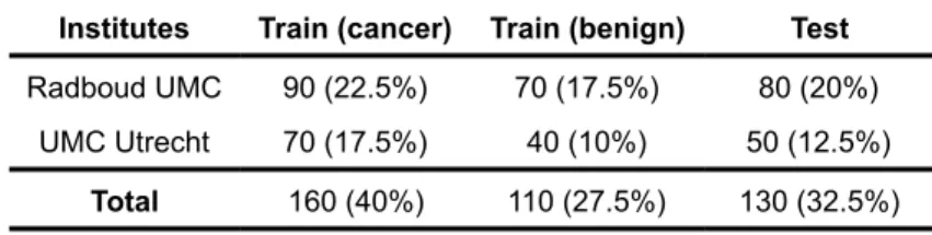
A study of the breast cancer detection used a novel approach of patch based classification followed by heatmap based postprocessing for generating tumor probability to detect metastatic breast cancer [ Wang et al., 2016 ]. The study emerged as one of the solutions from Camelyon16 ISBI challenge on cancer metastasis detection in lymph nodes (“CAMELYON16”, 2018) . The data was collected from two different institutes, Radboud University Medical Center (Nijmegen, the Netherlands), and the University Medical Center Utrecht (Utrecht, the Netherlands). Table 1. shows the data distribution.
Institutes Train (cancer) Train (benign) Test
Radboud UMC 90 (22.5%) 70 (17.5%) 80 (20%)
UMC Utrecht 70 (17.5%) 40 (10%) 50 (12.5%)
Total 160 (40%) 110 (27.5%) 130 (32.5%)
Table 1: Camelyon16 data distribution.
Two different evaluation metrics were used in this study: slidebased evaluation (SBE) and lesionbased evaluation (LBE). SBE was measured using ROCAUC score, based on the probabilities of each test slide containing cancer. LBE was measured using probability of a certain (x,y) pixel for each (predicted) cancer lesion for each whole slide image. The performance was measured as the average true positive rate for detecting all true cancer lesions in a wholeslide image (WSI) across 6 false positive rates: 0.25 , 0.5 , 1, 2, 4, and 8 false positives per WSI. As mentioned above the approach used in this study was two pronged, classification based on patch and headmap (postprocessing). Patchbased classification used WSI as input with the label, indicating ROI of each WSI containing metastatic cancer. Training was done using millions of small positive and negative patches, randomly generated from the training data. Patches in the ROI containing tumors were labeled positive otherwise negative. The postprocessing stage included tumor probability heatmap generation, the probability heatmap was further used to compute evaluation score based on both slide as well as lesion for each WSI. As opposed to developing a custom deep network from scratch, GoogleNet [ Szegedy et al., 2015 ] was the architecture of choice for training. The solution stood first in both competitions, with an impressive area under the receiver operating curve (AUC) of 0.925 for WSI classification and for tumor localization it achieved a score of 0.7051.
2.2 State of the Deep Neural Network Architectures
Since the problem area comes under the umbrella of image classification; therefore, it is of paramount importance to review the state of the art in image classification. The most prominent image classification solutions based on deep convolutional neural networks emerged as winners of the yearly Large Scale Visual Recognition Challenge (ILSVRC) [ Russakovsky et al., 2014 ]. Three architectures from the competition were chosen for this study.
2.2.1 Inception V1
In 2014, a research team from Google won the ILSVRC14. The codename of their architecture was inception [ Szegedy et al., 2015 ] . One of the key features of the solution was the improved utilization of computing resources. Conventionally, deep neural networks are deep only depthwise, this solution proposed a way to make the best use of depth as well as width on a constant computational budget. This architecture was inspired by networkinnetwork approach [ Lin et al., 2013 ] to boost the representational power of the network which is the very core of the inception module. One particular instance of this study is called GoogleNet consisting of layers. GoogleNet is very efficient in terms of memory and power use, for instance, a reflection of its efficiency is the fact that it takes 12 times lesser parameters as compared to Alexnet winner of [ “ILSVRC2012”, 2018 ].
At the heart of the GoogleNet is the inception module which is the core of the whole architecture. The inner working of this module is nontrivial. The module applies a 1x1 convolutional layer to already existing convolutional layers followed by linear activation [ Krizhevsky et al., 2012 ]. However, in inception, 1x1 convolution is multipurpose, it is mainly used for the purpose of dimensionality reduction and it allows not only to increase the depth, but also the width of networks, without affecting the performance so much. The inception architecture primarily focuses on dense components to efficiently map local sparse structures in a CNN. The architecture also takes inspiration from a layer by layer approach [ Arora et al., 2013 ] where it clusters units in groups with high correlation statistics in the last layer. Based on already perceived information that image patches in lower layers are highly correlated, these can be covered by 1x1 convolutions. Clusters that are spatially spreadout can be covered by applying bigger convolutions of 3x3 and 5x5, and patches decrease with the increase in region size. Also, it can be observed in the architecture that all the convolutional filters 1x1, 3x3 and 5x5 are concatenated before they are passed to the next layer, as illustrated in Figure 8.
GoogleNet won the 2014 ILSVRC with a 6.67% top5 error. The most successful version of GoogleNet (an incarnation of inception architecture) is described in Table 2. The first column contains the types of layers or modules used in the architectures. The ‘patch size/stride’ column describes the filter (patch) size along with stride size (height x width/stride), where applicable. The column ‘output size’ describes the output shape and size of each layer. The column ‘depth’ represents the depth of each layer/module. The column ‘# 1x1’ represents the number of 1x1 filters used in a specific layer. Similarly, columns ‘# 3x3’ and ‘# 5x5’ represent the number of 3x3 and 5x5 filters respectively. Columns ‘# 3x3 reduce’ and ‘# 5x5 reduce’ represent 1x1 filters applied before 3x3 and 5x5 filters respectively. The column ‘Pool proj’ represents the number of 1x1 filter applied after max pooling. Params and ops columns represent the number of parameters and operations per layer respectively. type patch size/ stride output size depth # 1x1 # 3x3 reduce # 3x3 # 5x5 reduce # 5x5 Pool proj params ops convolution 7 x 7 / 2 112 x 112 x 64 1 2.7K 34M max pool 3 x 3 / 2 56 x 56 x 64 0 convolution 3 x 3 / 1 56 x 56 x 192 2 64 192 112K 360M max pool 3 x 3 / 2 28 x 28 x 192 0 inception(3a) 28 x 28 x 256 2 64 96 128 16 32 32 159K 128M inception(3b) 28 x 28 x 480 2 128 128 192 32 96 64 380K 304M max pool 3 x 3 / 2 14 x 14 x 480 0 inception(4a) 14 x 14 x 512 2 192 96 208 16 48 64 364K 73M inception(4b) 14 x 14 x 512 2 160 112 224 24 64 64 437K 88M inception(4c) 14 x 14 x 512 2 128 128 256 24 64 64 463K 100M inception(4d) 14 x 14 x 528 2 112 144 288 32 64 64 580K 119M inception(4e) 14 x 14 x 832 2 256 160 320 32 128 128 840K 170M max pool 3 x 3 / 2 7 x 7 x 832 0 inception(5a) 7 x 7 x 832 2 256 160 320 32 128 128 1072K 54M inception(5b) 7 x 7 x 1024 2 384 192 384 48 128 128 1388K 71M avg. pool 7 x 7 / 1 1 x 1 x 1024 0 dropout(40%) 1 x 1 x 1024 0 linear 1 x 1 x 1000 1 1000K 1M softmax 1 x 1 x 1000 0 Table 2: GoogleNet incarnation of Inception architecture [ Szegedy et al., 2015 ].
2.2.3 InceptionV3
In 2016, researchers at Google published an improved version of inception architecture called InceptionV2 [ Szegedy et al., 2016 ] . The idea behind the improvement is to disintegrate the convolutions in the inception module even further. The idea was further refined in revised version InceptionV3. InceptionV3 first suggests 5x5 convolutions to be are replaced by consecutive 3x3 convolutions and then it introduces the idea of factorising the 3x3 convolutions even further into asymmetric convolutions of nx1. Moreover, it introduces the
concept of batch normalised auxiliary classifier of fully connected layers. Figure 3. illustrates the architecture of InceptionV3 network. The study suggests four design principles based on large scale experimentation on a wide variety of deep convolutional neural networks, the principles are as follows:
➢ While designing an architecture, avoid too much data compression in the earlier layers. In general the compression of data representation should take place uniformly as we move towards the output.
➢ In order to increase the training efficiency of a network, high dimensional data can be processed locally to retrieve segregated features by increasing activation per tile in a convolutional network.
➢ Dimensionality reduction, before spatial aggregation, is more efficient. The reason for that is believed to be the high correlation between adjacent units, which results in much less loss of information during dimensionality reduction.
➢ Striking a balance between the dimensions of the network, in terms of width and depth. A network can be optimized for performance by balancing the number of filters per stage and its depth.
The improvements in the actual inception architecture were brought about using the same design principles. Variants of InceptionV3 modules are illustrated in Figure 9.
Figure 9: Inception modules [ Szegedy et al., 2016 ].
Inception module A in Figure 9, shows a replacement of the one of the first inception modules where 5x5 convolutions are replaced by two 3x3 convolutions. Inception module B factorizes the nxn convolutions to 1xn and nx1 according to the third design principle. Finally, Inception module C represents the second design principle, locally processing high dimensional data by spatial aggregation (1x1 convolutions).
Table 3. provides an abstracted representation of the architecture of the proposed network. It makes use of the inception modules in Figure 9.
type patch size/stride or remarks Input size conv 3x3/2 299x299x3 conv 3x3/1 149x149x32 conv padded 3x3/1 147x147x32 pool 3x3/2 147x147x64 conv 3x3/1 73x73x64 conv 3x3/2 71x71x80 conv 3x3/1 35x35x192 3 x Inception Inception module A 35x35x288 5 x Inception Inception module B 17x17x768 2 x Inception Inception module C 8x8x1280 pool 8 x 8 8x8x2048 linear logits 1x1x2048 softmax classifier 1x1x1000 Table 3: InceptionV3 model [ Szegedy et al., 2016 ].
The column ‘type’ contains all layers/modules used in the architecture. The column ‘patch size/stride or remarks’ contains information regarding filter size, step size and if applicable remarks about the corresponding layers. ‘Input size’ represents the input dimensions of the layer/module: height x width x filtercount.
InceptionV3 was trained and tested on ILSVRC12 data and it achieved 21.2% top1 and 5.6% top5 error for single crop evaluation.
2.2.4 Xception
In 2015, Francois Chollet, an artificial intelligence researcher at Google and the developer of the famous neural network python API Keras, proposed yet another deep neural network architecture called Xception. It was inspired by the inception modules. In his study he broke down the interpretation of inception module as in intermediary between normal convolutions and depthwise separable convolution operation, which eventually lead to the ideation of a novel deep convolutional neural network architecture. The depthwise separable convolutions are at the heart of this architecture. [ Chollet, 2016 ].
The advent of inceptionlike architecture was a paradigm shift from Visual Geometry Group (VGG) style [ Simonyan & Zisserman, 2014 ] architecture. VGG style networks were primarily stacks of simple convolutional layers, whereas inceptionlike architectures used inception modules as building blocks. Although, inception modules bear conceptual similarity to convolution, they learn a far richer representation of data with less parameters. The power of inception module lies in the decoupling of spatial and crosschannel correlations. Xception architecture pushed the boundaries even further by introducing depthwise separable convolutions, which is similar to the idea of extreme inception: to
separately map spatial correlations for each channel. However, they differ from each other in two ways
➢ Inception performs 1x1 convolution first, whereas depthwise separable convolution performs channelwise spatial convolution first.
➢ In inception, both operations are followed by piecewise linearity, rectified linear unit (ReLu), whereas depthwise convolutions do not strictly rely on piecewise linearity. An abstract representation of the Xception architecture is described in Figure 10. Figure 10: Xception architecture [ Chollet, 2016 ].
Conceptually, Xception architecture is distributed into 3 main parts: entry flow, middle flow and exit flow. The data is first passed through the entry flow, then iteratively processed 8 times through the middle flow, and finally passed through the exit flow. In this process flow, batch normalization is performed on the data after every Convolution and SeparableConvolution layer, which is explicitly shown in Figure 10. Each SeparableConvolution employs a depth multiplier of 1.
Xception architecture was compared with InceptionV3 architecture on a large image classification dataset comprising of 350 million images and 17,000 classes. Since both architectures have the same number of input parameters, the improved performance of Xception is the result of model efficiency. Xception achieved a top1 accuracy of 0.790 and top5 accuracy of 0.945.
2.2.5 Deep Residual Learning for Image Recognition
Residual networks brought back very deep convolutional networks back to limelight. In 2015, researchers at Microsoft proposed the idea of deep residual learning for image recognition [ He et al., 2015] . The idea was to use residual blocks as the core concept of the network to tackle vanishing and exploding gradients in order to improve the learning process of the network. It became evident from experiments that this approach not only made it easier to optimize the network, but yielded better accuracy with increased depth as well. These networks were significantly deeper than their predecessors in deep networks such as VGG nets [ Simonyan & Zisserman, 2014 ]. One incarnation of residual networks has 152 layers which is 8x the depth of VGG nets.
At the heart of residual network, there is the residual block. In a nutshell, the function of a residual block is to perform an identity mapping through a skip connection. In this residual learning framework, the idea is to explicitly let the layers fit a residual mapping instead of relying on stacked layers to directly fit a desired mapping. Let the desired underlying mapping of the residual be H(x). We set the residual block such that H(x) = F(x) + x where F(x) is linear product of the residual block and x is the identity mapping, H(x) is the combined output of these two. Figure 11 graphically represents a residual block.
Figure 11: Residual Learning: a building block [ He et al., 2015 ].
A combination of these residual networks achieved 3.57% error on the ImageNet test dataset, securing first position in ILSVRC 2015 classification task. Due to the deep representation of residual networks, the solution gained 28% improvement on the COCO dataset. A 34layer residual network is illustrated in Figure 12. The architecture starts with a layer containing 64 ‘7x7’ convolution filters and then it is further divided into 4 parts, the first uses layers with 64 ‘3x3’ convolution filters, the second part uses layers with 128 ‘3x3’ convolution filters, the third part uses layers 256 ‘3x3’ convolution filters and the fourth part uses layers with 512 ‘3x3’ filters. The fourth part is followed by a fully connected dense layer with 1000 neurons.
Altogether, the network consists of 34 layers. The residual block in Figure 11 is the building of block of the network.
3. DATASET AND FRAMEWORKS
3.1 Dataset
The dataset used in this thesis work was made public in a 2017 online competition called ProstateX2 [“SPIEAAPMNCI Prostate MR Gleason Grade Group Challenge”, 2018]. The dataset comprised of mpMRI scans of 99 patients. The mpMRI scans had four different modalities: ➢ T2weighted transaxial images (DICOM format). ➢ T2weighted sagittal images (DICOM format). ➢ Ktrans images (mhd format) ➢ Apparent diffusion coefficient (ADC) images (DICOM format).
These cases contained 112 lesions. Each lesion had a known pathologydefined Gleason Grade Group [ Epstein et al., 2016 ]. The total Gleason score (GS) was calculated based on the appearance of the cells under the microscope, the first half of the score was the representation of most common cell morphology, and the second half was the second most common cell pattern. Both halves score ranged from 1 to 5. Gleason grade groups are illustrated in Figure 13 and are following:
Gleason Grade Group 1 (GS less than 6): Wellformed separable glands.
Gleason Grade Group 2 (GS 7[3+4]): Mainly wellformed glands with sporadic presence of poorlyformed glands as the smaller component.
Gleason Grade Group 3 (GS 7[4+3]): Mainly poorlyformed or fused glands with sporadic presence of wellformed glands as the smaller component.
Gleason Grade Group 4 (GS 8[4+4]; 8[3+5]; 8[5+3]): (1) Only poorlyformed glands or (2) mainly wellformed glands and lacking glands as the smaller component or (3) mainly lacking glands and the smaller component of wellformed glands.
Gleason Grade Group 5 (GS 9 or 10) : There is dearth of gland formation in this group including or excluding poorlyformed glands.
Gleason grade group 2 and 3 both had a total score of 7, however, they differed depending on the scores of the most common and second most common cell morphology. [“SPIEAAPMNCI Prostate MR Gleason Grade Group Challenge”, 2018].
Figure 13: Gleason grade groups [ “How is Prostate Cancer Diagnosed?”, 2018 ].
3.1.1 Exploratory Analysis
Exploratory analysis of data included basic visualisation techniques to understand the scans better. These visualisations included, region of interest detection, analysis of zone information distribution and Gleason grade group distribution. Exploratory analysis helped in detecting class imbalance, random order of prostate slices (which was fixed by reading the metadata from DICOM headers), lack of standardization of image resolution across different cases as well as modalities. Figure 14 shows region of interest highlighted with a red bounding box in four different image artifacts.
Figure 14: T2 weighted scan (sagittal and transaxial plane), apparent diffusion coefficient and bvalue scan with ROI highlighted with a red bounding box.
Figures 15 & 16 show the distribution of zone information and Gleason grade group, respectively.
Figure 15: Bar chart showing zone information distribution, AS: anterior fibromuscular stroma, PZ: peripheral zone, TZ: transition zone. Figure 16: Pie chart showing Gleason grade groups distribution.
![Figure 5: Generating a threechannel RGB image from three mpMRIs [ Tsehay et al., 2017 ].](https://thumb-us.123doks.com/thumbv2/123dok_us/9789471.2470704/18.893.246.647.799.1075/figure-generating-three-channel-image-three-mris-tsehay.webp)
![Figure 7: Comparison of real and synthetic ROI patches [ Kitchen & Seah, 2017 ].](https://thumb-us.123doks.com/thumbv2/123dok_us/9789471.2470704/21.893.131.766.178.1034/figure-comparison-real-synthetic-roi-patches-kitchen-seah.webp)
![Figure 9: Inception modules [ Szegedy et al., 2016 ].](https://thumb-us.123doks.com/thumbv2/123dok_us/9789471.2470704/26.893.133.780.577.865/figure-inception-modules-szegedy-et-al.webp)
![Figure 11: Residual Learning: a building block [ He et al., 2015 ].](https://thumb-us.123doks.com/thumbv2/123dok_us/9789471.2470704/29.893.314.585.730.874/figure-residual-learning-building-block-he-et-al.webp)
![Figure 12: 34Layer Resnet [ He et al., 2015 ].](https://thumb-us.123doks.com/thumbv2/123dok_us/9789471.2470704/30.893.389.534.192.1114/figure-layer-resnet-he-et-al.webp)
![Figure 13: Gleason grade groups [ “How is Prostate Cancer Diagnosed?”, 2018 ].](https://thumb-us.123doks.com/thumbv2/123dok_us/9789471.2470704/32.893.248.635.116.638/figure-gleason-grade-groups-how-prostate-cancer-diagnosed.webp)