Multilabel Classifiers with a Probabilistic Thresholding
Strategy
Jos´e Ram´on Quevedo, Oscar Luaces∗, Antonio Bahamonde Artificial Intelligence Center
University of Oviedo at Gij´on, Asturias, Spain
Abstract
In multilabel classification tasks the aim is to find hypotheses able to predict, for each instance, a set of classes or labels rather than a single one. Some state-of-the-art multilabel learners use a thresholding strategy, which consists in computing a score for each label and then predicting the set of labels whose score is higher than a given threshold. When this score is the estimated posterior probability, the selected threshold is typically 0.5.
In this paper we introduce a family of thresholding strategies which take into account the posterior probability of all possible labels to determine a different threshold for each instance. Thus, we exploit some kind of interde-pendence among labels to compute this threshold, which is optimal regarding a given expected loss function. We found experimentally that these strate-gies outperform other thresholding options for multilabel classification. They provide an efficient method to implement a learner which considers the in-terdependence among labels in the sense that the overall performance of the prediction of a set of labels prevails over that of each single label.
Keywords: Multilabel Classification, Thresholding Strategies, Posterior Probability, Expected Loss
∗Corresponding author: Tel: +34 985 182 032
Email addresses: [email protected](Jos´e Ram´on Quevedo),
[email protected](Oscar Luaces),[email protected](Antonio Bahamonde)
1. Introduction
Let L be a finite and non-empty set of labels or classes. In a multiclass
classification task involving L, each input instance has only one single label or class belonging to L. In multilabel classification, however, a subset of labels or classes is attached to each instance.
This kind of classification arise in different fields. In many databases, text documents, videos, music or movies are tagged with several labels. In biology, the description of the functionalities of genes frequently requires more than one label. Tsoumakas and Katakis [1] have made a detailed presentation of multilabel classification and their applications.
Recently, multilabel classification has received increasing attention due to its applications and also because of its own appeal as an intellectual challenge. Usually, the goal is to find a way to take into account the correlation or interdependence between labels. In fact, it is possible to tackle a multilabel classification task by simultaneously learning one binary classifier for each label. However, these binary classifications are not entirely independent. The presence or absence of a label in the set of labels assigned to an instance may be conditioned by other labels. The aim of a multilabel approach is to predict a set of labels as opposed to a simultaneous bunch of independent binary predictions.
Some state-of-the-art methods that follow this approach produce, for each instance, a score for each label inL[2, 3]. Moreover, in some interesting cases, the scores of labels are estimations of their posterior probabilities [4, 5, 6]. Once we have a score or a ranking, a set of labels can be obtained using a threshold. Typically, the threshold for posterior probabilities in probabilistic methods is 0.5. However, thresholding can be more sophisticated. Ioannou et al. [7] report a theoretical and empirical comparative study of existing thresholding methods.
Thresholding can be considered as a method to adopt a global approach from the point of view of the set of labels; in fact, the threshold is selected taking into account the scores of all the labels. Once a threshold is fixed for a given input instance, the prediction is the set of labels with a higher score. Threshold computations must thus consider the consequences of predicting a set of labels rather than just the individual effects of including each one. Thresholding strategies are frequently effective and mostly efficient multilabel learners.
on optimizing the expected loss for a given loss function, we call these strate-gies Probabilistic Thresholds (PT). They can be considered as an extension of the so-called nondeterministic classifiers [8, 9] to multilabel instead of multiclass classification tasks.
The computational cost of PT is very low, but they produce a dramatic improvement when the performance is measured by functions like F1 or the
Accuracy, functions for which it is acknowledged that a global approach is useful. However, no improvements can be made if we use the Hamming loss, the average of 0/1 errors of the binary classifiers of each label. This fact was noted by Dembczy´nski et al. [5].
After a detailed description of PT, the paper includes an experimental comparison of these strategies with other options previously described in the literature. The result is that the PT family significantly outperforms all alternative thresholding strategies.
2. Formal Framework for Multilabel Classification
Let Lbe a finite and non-empty set of labels {l1, . . . , lm}, and let X be an input space. Let D={(x1,Y1), . . . , (xn,Yn)} be a dataset consisting of instances described by pairs (xi,Yi), where xi ∈ X and Yi ⊂L is a subset of labels. The goal of a multilabel classification task is to induce from D a hypothesis, which is a function from the input space X to the power set of labels P(L),
h:X −→P(L).
Multilabel classification can be seen as a kind of Information Retrieval task for each instance, in which the labels play the role of documents. The predictionh(x) can thus be understood as the set ofrelevantlabels retrieved for a query x.
Performance in Information Retrieval is compared using different mea-sures in order to consider different perspectives. The most frequently used measures are Recall (proportion of all relevant documents (labels) that are found by a search) and P recision (proportion of retrieved documents (la-bels) that are relevant). The harmonic average of the two amounts is used to capture the goodness of a hypothesis in a single value. In the weighted case, the measure is calledFβ and constitutes a trade-off betweenRecall and
P recision.
For further reference, let us recall the formal definitions of these measures. Thus, for a prediction of a multilabel hypothesis h(x) and a subset of truly
relevant labelsY ⊂L, we can compute the following contingency matrix:
Y L\Y
h(x) a b
L\h(x) c d
(1)
in which each entry (a, b, c, d) is the number of labels in the intersection of the corresponding sets of the row and column. Notice for instance, that a is the number of truly relevant labels predicted by hforx; i.e.,a=|h(x)∩Y|.
According to matrix (1), we thus have the following definitions.
Definition 1. The Recall in a query (i.e., an instance x) is defined as the proportion of truly relevant labels, Y, included in h(x):
R(h(x),Y) = a
a+c =
|h(x)∩Y|
|Y| . (2)
Definition 2. The Precision is defined as the proportion of retrieved labels in h(x) which are truly relevant:
P(h(x),Y) = a
a+b =
|h(x)∩Y|
|h(x)| . (3)
Finally, the trade-off is formalized by
Definition 3. The Fβ (β≥0) is defined, in general, by
Fβ(h(x),Y) =
(1 +β2)P R β2P +R =
(1 +β2)a
(1 +β2)a+b+β2c. (4)
The most frequently used F-measure is F1. For ease of reference, let us
state the formula of F1 for a pair (h(x),Y):
F1(h(x),Y) =
2·a
2·a+b+c =
2|h(x)∩Y|
|Y|+|h(x)|. (5)
Other frequently used measures of the performance of multilabel classi-fiers can also be defined using the contingency matrix (1). This is the case of the Accuracyand Hamming loss defined as follows.
Definition 4. The Accuracy in a pair (h(x),Y) is defined by Tsoumakas and Katakis [1] as the proportion
Ac(h(x),Y) = a
a+b+c =
|h(x)∩Y|
|h(x)∪Y|. (6)
Definition 5. TheHamming lossin a pair (h(x),Y) is defined by Tsoumakas and Katakis [1] as the proportion of labels in the symmetric difference ofh(x) and Y
Hl(h(x),Y) = b+c |L| =
|h(x)∆Y|
|L| . (7)
In the experiments reported at the end of the paper, we micro-averaged
F1, the Accuracy and Hamming loss across the examples of a test set D0.
For ease of reading these scores are expressed as percentages. However, to be expressed as loss functions, we must consider that F1 and the Accuracy
are monotone with respect to the quality of the hypotheses and they have values in the interval [0,100]. Hence, the corresponding loss functions must be given by the difference with 100. Naturally, this is not necessary for the
Hamming loss.
For further reference, we provide here the expressions of the loss functions defined above given a family of contingency matrices{(ai, bi, ci) :i= 1, ..., n0} for each element of a set D0 ={(x01,Y01), . . . ,(x0n0,Y0
n0)}. LF1(h, D 0 ) = 100− 100 |D0| |D0| X i=1 2|h(x0i)∩Y0i| |Y0 i|+|h(x0i)| = 100− 100 |D0| |D0| X i=1 2ai 2ai+bi+ci (8) LAc(h, D0) = 100− 100 |D0| |D0| X i=1 |h(x0i)∩Y0i| |h(x0i)∪Y0i| = 100− 100 |D0| |D0| X i=1 ai ai+bi +ci (9) LHl(h, D0) = 100 |D0| |D0| X i=1 |h(x0i)∆Y0i| |L| = 100 |D0| |D0| X i=1 bi+ci |L| . (10)
There are other loss functions mentioned in the literature on multilabel classifiers that are not defined using contingency matrices [1, 4]. These are typically measures based on the ordering or preferences of the set of labels attached to an instance. We shall not deal with these measures in this paper.
3. Probabilistic Multilabel Classifiers and Thresholding Strategies
There is a straightforward approach to cope with a multilabel classifica-tion task, which consists in decomposing it into as many binary classificaclassifica-tion tasks as the original problem has labels. This decomposition procedure, known as Binary Relevance (BR), requires learning an independent binary classifier for each label l ∈ L that will predict its inclusion (or not) in the final multilabel solution, for each instance x∈ X,
hl(x)∈ {0,1},∀l ∈L.
If these classifiers are based on the estimation of posterior probabilities, we have
Pr(l|x),∀l∈L,x∈ X. (11)
Thus, a multilabel hypothesis can be defined in terms of the posterior probabilities by
h(x) = {l∈L:hl(x) = 1}={l∈L: Pr(l|x)>0.5} ⊂L. (12) Some state-of-the-art multilabel learners try somehow to explicitly con-sider the correlation or interdependence between labels [3, 4, 5, 6]. The difference with respect to BR is the way they compute the posterior proba-bilities for each label given an instance x, but even in such cases the set of predicted labels is determined by (12).
In this paper we assume that we have learned estimations of posterior probabilities. The aim is to explore the consequences of changing the constant value 0.5 in (12) into a more general expression θ that may depend on the instance x. This is called a thresholding strategy[7], the formal definition of which is given by
hθ(x) ={l ∈L: Pr(l|x)> θ(x)} ⊂L. (13) There is another possible way to define a thresholding strategy. Given
x, we assume that the set of labels is ordered according to their posterior probabilities, i.e.,
The threshold may thus be defined by an integer function r that, in general, will depend on the instance x. Hence, the prediction is the set ofr(x) labels with the highest posterior probabilities:
hr(x) ={l1, l2, . . . , lr(x)} ⊂L. (15)
In any case, it is worth noting that a different threshold can be selected for each instance depending on the posterior probabilities of the whole set of possible labels. In other words, a label will be predicted for each instance that depends not only on its own probability, but also on the probabilities of the other labels. In this sense, thresholding enables a learner to take into account the interdependence between labels. More formally, the thresholds of (13) and (15) have the following general form:
θ(x) = θ(Pr(l|x) :l ∈L) (16)
r(x) = r(Pr(l|x) :l∈L). (17) There is an interesting study about thresholding strategies [7], in which the authors conclude that the most powerful strategies are OneThreshold
(OT) and Metalearner (Meta). In OT, the threshold function θ of Eq. (13) is constant: it does not depend on the instancex. Read et al. [10] used cross-validation to determine the value of the thresholdθ, while a computationally simpler approach was followed in [3].
In the work of Tang et al. [11]Metawas implemented using (15), in which
r(x) was an estimation of the number of labels for instance x, which was learned as a multiclass classification task. These authors estimated posterior probabilities by means of a BR learner built from a binary classifier based on LibLinear [12, 13].
Notice that neitherOT nor Metarequire posterior probabilities. In fact, they can be applied to classifiers providing any kind of score function.
4. Optimizing the Expected Loss with a Thresholding Strategy
In this section we present a new thresholding strategy based on the es-timation of the expected loss measured by a function of the contingency matrix (1). Let us recall that we assume that, for each instance, we have estimations of posterior probabilities for each label (11).
The core idea can be seen as an extension of nondeterministic classifiers [8, 9] to multilabel classification tasks. In nondeterministic classifiers, the
aim is to widen the prediction in doubtful situations from one single class to a subset of classes in order to increase the probability of achieving a success-ful prediction, while keeping a reduced number of classes in the prediction, seeing as we know the true output is a single class. The extension to multil-abel classification consists in determining the most promising threshold with respect to a given loss function so as to predict a subset of labels. In this case, however, we are not considering the number of expected labels to be predicted. The reason is that the true relevant labels for an instance, un-fortunately, do not always occupy the first places in the ranking given by posterior probabilities.
Throughout this section, we shall assume thatx is an instance and that the set of labels is ordered according to their posterior probabilities as in (14).
Definition 6. Let L be a function that depends on a contingency ma-trix (1). Given an instance x, the expected loss, measured by L, of a hypothesis that predicts the r labels with the highest posterior probabilities is
∆r(x) =
X
a,b,c
L(a, b, c)·Pr(a, b, c|r,x). (18) Notice that entry d of the contingency matrix is not needed given that
d =|L| −(a+b+c). Moreover, Equations (8), (9), and (10) are defined in terms of {a, b, c}.
To build a hypothesis with the lowest expected loss within this context, we need to estimate ∆r(x) for eachrin order to make the following definition.
Definition 7. The thresholding strategy for an instance x with the lowest expected loss L, calledProbabilistic Thresholding (P TL), is given by
P TL(x) ={l1, . . . , ls|s=
|L|
arg min r=1
∆r(x)} (19)
Notice that we can optimize micro-averages of F1 (8), the Accuracy (9),
or Hamming loss (10) if we can estimate ∆r(x).
4.1. Algorithm of the Probabilistic Thresholding Strategy
To present an algorithm for a probabilistic thresholding strategy that aims to optimize a loss function L, we shall first introduce a method to estimate ∆r(x) in (18) using the notation of the preceding sections.
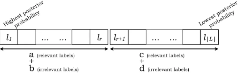
lr+1 ... ... l|L| l1 ... ... lr a (relevant labels) + b (irrelevant labels) c (relevant labels) + d (irrelevant labels) Highest poster ior probability Lowest poster ior probability
Figure 1: Given an instance x, if the labels are ordered according to their posterior probabilities andris an integer between 1 and|L|, we need to estimate the probability of havinga(respectively,c) relevant labels forxin the firstrlabels (respectively, in the set of labels placed from positionsr+ 1 to|L|).
For this purpose, we need the probability of all possible contingency ma-trices for a given instance. However, note that the variables involved in these matrices are closely related; for instance, b =r−a. If [[predicate]] represents the value 1 when the predicate is true and 0 otherwise, then we have that
Pr(a, b, c|r,x) = Pr(a, c|r,x)·[[b=r−a]] = (20) = Pr(c|a, r,x)·Pr(a|r,x)·[[b =r−a]].
If we arrange the labels in descending order according to their posterior probabilities given x, then we can define a function
Px(rl, f, t), rl ∈ {0,1, . . . ,|L|}, f ∈ {1,2, . . . , t}, t∈ {1,2, . . . ,|L|}, to estimate the probability of having exactlyrlrelevant labelsfrom positionf
to positiontin the sorted list of labels. Notice that usingPx, the probability of a given contingency matrix in (20) can be expressed (see also Figure 1) as Pr(a, b, c|r,x) =Px(c, r+ 1,|L|)·Px(a,1, r)·[[b=r−a]]. (21) To approximate Px we shall assume that the posterior probabilities of different ranking positions are independent. We can thus formulate the fol-lowing recursive definition:
Px(rl, f, t) = Pr(lf|x)·Px(rl−1, f + 1, t)+ +(1−Pr(lf|x))·Px(rl, f+ 1, t) ifrl >0∧f < t; (22a) (1−Pr(lf|x))·Px(rl, f+ 1, t) ifrl= 0∧f < t; (22b)
Additionally, this definition needs some base cases; we define the follow-ing: Base cases Px(0, t, t) = 1−Pr(lt|x) (23a) Px(1, t, t) = Pr(lt|x) (23b) Px(rl, t, t) = 0; rl≥2 (23c)
The rationale of this function is quite straightforward. The probability of having rl >0 relevant labels in a list is given by (22a), which computes a weighted sum of the probabilities of being relevant and not relevant for the first label. Both probabilities are weighted by the probability (recursive call) of having the remaining relevant labels in the rest of the list, i.e., (rl−1) and rl respectively.
In turn, the probability of having no relevant labels in a list (22b) is the probability of the first one not being relevant times the probability of having zero relevant labels in the rest of the list.
The base cases represent the probability of having relevant labels in a list with just one label. Thus, the probability of having 0 relevant labels (23a) is the complementary of having one (23b). Finally, in (23c) the probability is 0 since it is impossible to have more than one relevant label in a list with just one label.
Moreover, note that the third argument of Px is constant throughout the previous recursive definition. Thus, having fixed a value t >0, we may discard this argument. Px can thus be computed using a dynamic program-ming algorithm. Figure 2 sketches an iterative procedure that may be used to compute this function. Once we have an estimation of the expected loss, given an instance xwe define the probabilistic thresholding strategy of (19) using Algorithm 1.
4.2. Complexity
The implementation of thePT strategy calculates for each possible thresh-old, i.e., for each possible number of predicted labels r≤ |L|, the probability of each contingency matrix and its corresponding loss, as required by (18).
Thus, for each value ofr, all contingency matrices have only two degrees of freedom given that a+b = r and a+b+c+d = |L| (see Figure 1 and Equation (20)). The probability of each contingency matrix is estimated by
0 1 2 |L| 1 0 (1–Pr(lt-1|x)) ! Pr(lt-1|x) ! +(1–Pr(lt-1|x)) !
⋰
⋮
t 1–Pr(lt|x) Pr(lt|x) 0 0rl
f
Figure 2: To computePx(rl, f, t) according to the definition of (22), using the base cases
of (23) and for a fixedt >0, we may use a dynamic programming algorithm to complete this matrix of values iteratively. The dashed lines indicate the dependency in the recursive definition.
means of the function Px(rl, f, t), defined in (22) and (23), which is imple-mented using a dynamic programming algorithm that iterates through the values of rland f to fill the matrix depicted in Figure 2.
The time complexity of this filling process is O(|L|2), since the
dimen-sion of the matrix is t× |L|, where t ≤ |L|. Therefore, O(PT) = O(|L|)· (O(L(a, b, c)) +O(|L|2)). When O(L(a, b, c)) = 1, as in typical loss
func-tions like F1, the Accuracy or Hamming loss, we have that O(PT) =O(|L|)·(1 +O(|L|2)) =O(|L|3).
5. Experimental Results
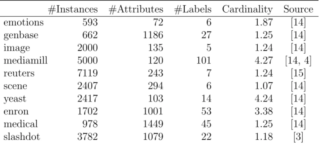
In this section we present an experimental comparison carried out to validate the proposals set out in this paper. We used 10 datasets which have been employed in previous publications on multilabel classification. Table 1 shows a summarized description of these datasets, including references to their sources.
In all cases we estimate the performance of learners by means of 10-fold cross-validations. The scores reported are the micro-averaged F1, the
Algorithm 1 Given an instance x and the posterior probabilities of all labels, this algorithm computes the thresholding strategy that minimizes the expected loss for a function (L) that depends on the contingency matrix (1).
Input: object description x Input: {Pr(li|x) :i= 1, ..,|L|}
order the set of labels L={l1, ..., l|L|} according to Pr(li|x); best.r = 0; best.loss = ∞; for r = 1 to|L| do loss= 0; for a= 0 to r do for c= 0 to |L| −r do b=r−a; loss+= L(a, b, c)·Px(c, r+ 1,|L|)·Px(a,1, r); end for end for
if (loss < best.loss)then best.r=r;best.loss=loss end if end for
return {l1, . . . , lbest.r};
Accuracy and Hamming loss obtained using 3 base learners with different thresholding strategies.
We used OneThreshold (OT) and Metalearner (Meta); see Section 3. In the case of OT, we considered three different versions to optimize F1, the
Accuray and Hamming loss, named respectively OTF1, OTAC, and OTHl;
the implementation was carried out with an internal 5-fold cross-validation following the work of Read et al. [10].
These strategies were compared with theProbabilistic Thresholdingsthat aim to optimize the 3 measures considered; the multilabel classifiers so ob-tained were called P TF1, P TAC, and P THl.
As base learners, we used 3 different multilabel learners to compute pos-terior probabilities.
• First, a Binary Relevance (BR) logistic regressor implemented with
LibLinear [12, 13] with the default value for its regularization param-eter C = 1. The implementation was performed in Matlab using an interface with LibLinear.
#Instances #Attributes #Labels Cardinality Source emotions 593 72 6 1.87 [14] genbase 662 1186 27 1.25 [14] image 2000 135 5 1.24 [14] mediamill 5000 120 101 4.27 [14, 4] reuters 7119 243 7 1.24 [15] scene 2407 294 6 1.07 [14] yeast 2417 103 14 4.24 [14] enron 1702 1001 53 3.38 [14] medical 978 1449 45 1.25 [14] slashdot 3782 1079 22 1.18 [3]
Table 1: The datasets used in the experiments; some associated statistics.
implementation provided by the authors through the library Mulan
[14, 16], which is built on top ofWeka[17]. We wrote an interface with Matlab to ensure that cross-validations were carried out with the same splits of training and testing data.
• The third multilabel learner was the Ensembles of Classifier Chains (ECC)[3] in the version used by Dembczy´nski et al. [5]; for this reason we called it ECC*. The implementation was carried out using the BR
built with LibLinear.
5.1. Comparison of Results
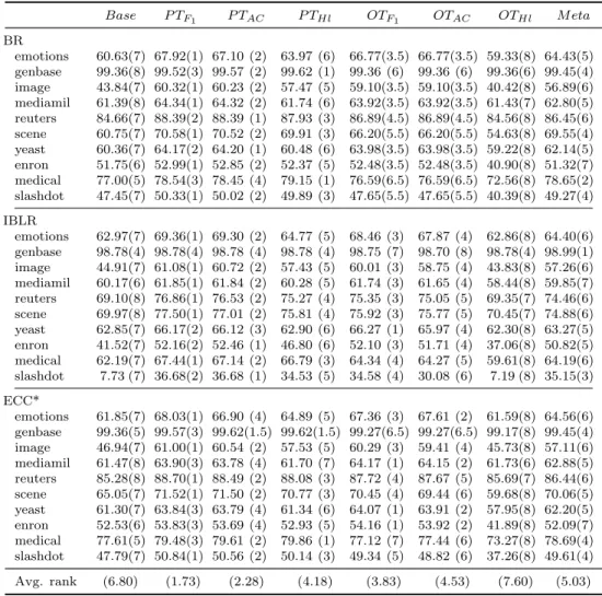
Tables 2, 3, and 4 respectively report the scores obtained by base learners and the thresholding strategies considered inF1, theAccuracyandHamming
loss. In addition to cross-validation values, we report, between brackets, the relative ranking positions achieved by each classifier in each dataset. The last row of the tables displays the average ranking position of each learner.
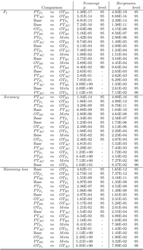
Following the recommendations of Demˇsar [18] and Garc´ıa and Herrera [19], we performed a two-step comparison for each of the considered measures. The first step is a Friedman test that rejects the null hypothesis: not all learners perform equally. For this purpose, we considered all base learner scores together, since the objective was to compare different thresholding strategies, not base learner scores.
The second step is apost-hoc pairwise comparison. Following Garc´ıa and Herrera [19], we performed a Bergmann-Hommel’s procedure using the soft-ware provided in their paper. This comparison is preferred to the use of
Nemenyi’s test, recommended by Demˇsar [18], because it is a very conser-vative procedure and many of the obvious differences may not be detected. In any case, we report the results of both tests. We modified the output of Garc´ıa and Herrera’s p-values for Nemenyi’s test, multiplying them by the number of pairs compared; thus, the threshold for the standard confidence levels, 90% and 95% are, respectively α= 0.05 andα = 0.1.
The p-values of the significant pairwise comparisons are reported in Ta-ble 5. To facilitate interpretation of these taTa-bles, we include a graphical representation of the comparison using Bergmann’s procedure. The graphs are shown in Figure 3.
5.2. Discussion
In all cases, Probabilistic Thresholds achieve scores that are not signifi-cantly worse than the scores of any other alternative approach in the com-parison. However, the results depend heavily on the loss function considered. For instance, the comparison ofHamming loss scores highlights the good performance of Base learners. None of the thresholding strategies is better than Base when using the Hamming loss. This is coherent with the results presented by Dembczy´nski et al. [5], in which the authors claim that multi-label methods may benefit with respect to some loss measures due to their ability to exploit some kind of interdependence among labels, but the gain, if any, will be much smaller for measures like Hamming loss. In any case, notice that, as expected, the best thresholding strategies are those devised to optimize Hamming loss.
On the other hand, thresholding strategies optimizingF1 or theAccuracy
clearly outperform base learners in such measures. In fact, the classifiers obtained in both cases seem to be quite similar. Recall that the loss functions in (5) and (6) are quite similar, too. Thus, P TF1 occupy the first place in
F1, but the second position is forP TAC with no significant differences. Both strategies significantly outperform all the others.
When comparing accuracy scores, P TAC is the best strategy, although
P TF1, and even P THl, are not significantly different from P TAC. Moreover,
they are only significantly better than some of the other strategies. On the other hand, P TAC is significantly better than all OT and Meta strategies and, of course, better than Baselearners.
Additionally, the comparisons lead to the conclusion that F1 and
Ham-ming loss are somehow opposite optimization aims. Notice that in Fig-ure (3.iii), and in Table 5,P TF1 andOTF1 occupy the lowest positions; while
(i)
•
F1 Base(6.80) OTHl(7.60) OTAC(4.53) OTF1(3.83) PTHl(4.18) PTF1(1.73) PTAC(2.28) Meta(5.03) (ii)•
Accuracy Base(6.57) OTHl(7.63) OTAC(4.40) OTF1(5.00) PTHl(3.25) PTF1(3.00) PTAC(2.25) Meta(3.90) (iii)•
Hamming loss
Base(2.35) OTHl(2.50) OTAC(5.50) PTF1(6.48) PTAC(5.05) Meta(4.37) PTHl(2.65) OTF1(7.10)Figure 3: Graphical representation of significant differences at the 90% level using Bergmann’s procedure on the scores from Table 5. The upper graph representsF1 scores,
in Figure (3.i), P TF1 and OTF1 are significantly better thanP THl and OTHl,
respectively.
Another interesting result is the role played by Meta, which in all cases occupies a middle position in rankings. The reason is probably that the aim of copying the number of relevant labels is only suboptimal if it is not possible to obtain a perfect ordering of the labels; and it is even worse if predictions of the number of relevant labels are not reliable.
6. Conclusion
We have presented a new family of thresholding strategies based on pos-terior probabilities, Probabilistic Thresholds (PT), which are based on the estimation of the expected loss given a loss function.
The computational cost of PT is negligible since they only require the computation of a square matrix of probabilities of the same size as the number of labels.
We have proven experimentally that the scores achieved by thresholding strategies considerably improve the performance of state-of-the-art multil-abel learners, even when using simple strategies likeOne Threshold orMeta. However, PT strategies are significantly better when the aim is to optimize micro-averaged F1 or the Accuracy.
Our conclusion is that thresholding is an efficient way to implement multi-label learners that somehow takes into account the interdependence of multi-labels for each instance. In fact, thresholding employs a global viewpoint to decide on the set of labels to predict instead of the local approach adopted, for instance, by Binary Relevance multilabel learners.
However, although useful for certain loss functions likeF1or theAccuracy,
the exploitation of label interdependence seems to provide very little benefit to other such functions. This is the case of theHamming loss, as was pointed out by Dembczy´nski et al. [5]. The experiments reported here corroborate this fact: base learners achieve the best scores, though the scores are not significantly different to those obtained by strategies that aim to optimize the Hamming loss.
Acknowledgements
The research reported here is supported in part under grant TIN2008-06247 from the MICINN (Ministerio de Ciencia e Innovaci´on, Spain). We
would also like to acknowledge all those people who generously shared the datasets and software used in this paper, as well as the anonymous reviewers’ suggestions, which contributed to improve the quality of our work.
[1] G. Tsoumakas, I. Katakis, Multi label classification: An overview, In-ternational Journal of Data Warehousing and Mining 3 (2007) 1–13. [2] G. Tsoumakas, I. Katakis, I. Vlahavas, Random k-labelsets for
multi-label classification, IEEE Transactions on Knowledge Discovery and Data Engineering (2010).
[3] J. Read, B. Pfahringer, G. Holmes, E. Frank, Classifier chains for multi-label classification, in: Proceedings of European Conference on Ma-chine Learning and Knowledge Discovery in Databases (ECML-PKDD), LNAI, Springer, 2009, pp. 254–269.
[4] W. Cheng, E. H¨ullermeier, Combining instance-based learning and logis-tic regression for multilabel classification, Machine Learning 76 (2009) 211–225.
[5] K. Dembczy´nski, W. Cheng, E. H¨ullermeier, Bayes optimal multilabel classification via probabilistic classifier chains, in: Proceedings of the 27th International Conference on Machine Learning (ICML), Omnipress, 2010.
[6] M. Zhang, Z. Zhou, ML-kNN: A lazy learning approach to multi-label learning, Pattern Recognition 40 (2007) 2038–2048.
[7] M. Ioannou, G. Sakkas, G. Tsoumakas, I. Vlahavas., Obtaining biparti-tions from score vectors for multi-label classification, in: Proceedings of the 22nd International Conference on Tools with Artificial Intelligence, IEEE, 2010.
[8] J. J. del Coz, J. D´ıez, A. Bahamonde, Learning nondeterministic clas-sifiers, Journal of Machine Learning Research 10 (2009) 2273–2293. [9] J. Alonso, J. J. del Coz, J. D´ıez, O. Luaces, A. Bahamonde, Learning to
predict one or more ranks in ordinal regression tasks, in: W. Daelemans, B. Goethals, K. Morik (Eds.), Proceedings of the European Conference on Machine Learning and Principles and Practice of Knowledge Dis-covery in Databases (ECML PKDD), LNAI 5211, Springer, 2008, pp. 39–54.
[10] J. Read, B. Pfahringer, G. Holmes, Multi-label classification using en-sembles of pruned sets, in: Proceedings of the 8th IEEE International Conference on Data Mining, ICDM’08, IEEE, 2008, pp. 995–1000. [11] L. Tang, S. Rajan, V. Narayanan, Large scale multi-label classification
via metalabeler, in: Proceedings of the 18th international conference on World Wide Web, ACM, 2009, pp. 211–220.
[12] C.-J. Lin, R. C. Weng, S. S. Keerthi, Trust region Newton method for logistic regression, Journal of Machine Learning Research 9 (2008) 627–650.
[13] R. Fan, K. Chang, C. Hsieh, X. Wang, C. Lin, LIBLINEAR: A library for large linear classification, Journal of Machine Learning Research 9 (2008) 1871–1874.
[14] G. Tsoumakas, E. Spyromitros-Xioufis, J. Vilcek, I. Vlahavas, Mulan: A Java Library for Multi-label learning, Journal of Machine Learning Research 12 (2011) 2411–2414.
[15] M. Zhang, Z. Zhou, M3MIML: A maximum margin method for multi-instance multi-label learning, in: Eighth IEEE International Conference on Data Mining, ICDM’08, ACM, 2008, pp. 688–697.
[16] G. Tsoumakas, I. Katakis, I. Vlahavas, Mining multilabel data, In O. Maimon and L. Rokach (Ed.), Data Mining and Knowledge Discovery Handbook, Springer (2010).
[17] I. Witten, E. Frank, Data Mining: Practical Machine Learning Tools and Techniques, Morgan Kaufmann Pub, 2005.
[18] J. Demˇsar, Statistical comparisons of classifiers over multiple data sets, Journal of Machine Learning Research 7 (2006) 1–30.
[19] S. Garc´ıa, F. Herrera, An extension on statistical comparisons of clas-sifiers over multiple data sets for all pairwise comparisons, Journal of Machine Learning Research 9 (2008) 2677–2694.
Base P TF1 P TAC P THl OTF1 OTAC OTHl M eta BR emotions 60.63(7) 67.92(1) 67.10 (2) 63.97 (6) 66.77(3.5) 66.77(3.5) 59.33(8) 64.43(5) genbase 99.36(8) 99.52(3) 99.57 (2) 99.62 (1) 99.36 (6) 99.36 (6) 99.36(6) 99.45(4) image 43.84(7) 60.32(1) 60.23 (2) 57.47 (5) 59.10(3.5) 59.10(3.5) 40.42(8) 56.89(6) mediamil 61.39(8) 64.34(1) 64.32 (2) 61.74 (6) 63.92(3.5) 63.92(3.5) 61.43(7) 62.80(5) reuters 84.66(7) 88.39(2) 88.39 (1) 87.93 (3) 86.89(4.5) 86.89(4.5) 84.56(8) 86.45(6) scene 60.75(7) 70.58(1) 70.52 (2) 69.91 (3) 66.20(5.5) 66.20(5.5) 54.63(8) 69.55(4) yeast 60.36(7) 64.17(2) 64.20 (1) 60.48 (6) 63.98(3.5) 63.98(3.5) 59.22(8) 62.14(5) enron 51.75(6) 52.99(1) 52.85 (2) 52.37 (5) 52.48(3.5) 52.48(3.5) 40.90(8) 51.32(7) medical 77.00(5) 78.54(3) 78.45 (4) 79.15 (1) 76.59(6.5) 76.59(6.5) 72.56(8) 78.65(2) slashdot 47.45(7) 50.33(1) 50.02 (2) 49.89 (3) 47.65(5.5) 47.65(5.5) 40.39(8) 49.27(4) IBLR emotions 62.97(7) 69.36(1) 69.30 (2) 64.77 (5) 68.46 (3) 67.87 (4) 62.86(8) 64.40(6) genbase 98.78(4) 98.78(4) 98.78 (4) 98.78 (4) 98.75 (7) 98.70 (8) 98.78(4) 98.99(1) image 44.91(7) 61.08(1) 60.72 (2) 57.43 (5) 60.01 (3) 58.75 (4) 43.83(8) 57.26(6) mediamil 60.17(6) 61.85(1) 61.84 (2) 60.28 (5) 61.74 (3) 61.65 (4) 58.44(8) 59.85(7) reuters 69.10(8) 76.86(1) 76.53 (2) 75.27 (4) 75.35 (3) 75.05 (5) 69.35(7) 74.46(6) scene 69.97(8) 77.50(1) 77.01 (2) 75.81 (4) 75.92 (3) 75.77 (5) 70.45(7) 74.88(6) yeast 62.85(7) 66.17(2) 66.12 (3) 62.90 (6) 66.27 (1) 65.97 (4) 62.30(8) 63.27(5) enron 41.52(7) 52.16(2) 52.46 (1) 46.80 (6) 52.10 (3) 51.71 (4) 37.06(8) 50.82(5) medical 62.19(7) 67.44(1) 67.14 (2) 66.79 (3) 64.34 (4) 64.27 (5) 59.61(8) 64.19(6) slashdot 7.73 (7) 36.68(2) 36.68 (1) 34.53 (5) 34.58 (4) 30.08 (6) 7.19 (8) 35.15(3) ECC* emotions 61.85(7) 68.03(1) 66.90 (4) 64.89 (5) 67.36 (3) 67.61 (2) 61.59(8) 64.56(6) genbase 99.36(5) 99.57(3) 99.62(1.5) 99.62(1.5) 99.27(6.5) 99.27(6.5) 99.17(8) 99.45(4) image 46.94(7) 61.00(1) 60.54 (2) 57.53 (5) 60.29 (3) 59.41 (4) 45.73(8) 57.11(6) mediamil 61.47(8) 63.90(3) 63.78 (4) 61.70 (7) 64.17 (1) 64.15 (2) 61.73(6) 62.88(5) reuters 85.28(8) 88.70(1) 88.49 (2) 88.08 (3) 87.72 (4) 87.67 (5) 85.69(7) 86.44(6) scene 65.05(7) 71.52(1) 71.50 (2) 70.77 (3) 70.45 (4) 69.44 (6) 59.68(8) 70.06(5) yeast 61.30(7) 63.84(3) 63.79 (4) 61.34 (6) 64.07 (1) 63.91 (2) 57.95(8) 62.20(5) enron 52.53(6) 53.83(3) 53.69 (4) 52.93 (5) 54.16 (1) 53.92 (2) 41.89(8) 52.09(7) medical 77.61(5) 79.48(3) 79.61 (2) 79.86 (1) 77.12 (7) 77.44 (6) 73.27(8) 78.69(4) slashdot 47.79(7) 50.84(1) 50.56 (2) 50.14 (3) 49.34 (5) 48.82 (6) 37.26(8) 49.61(4) Avg. rank (6.80) (1.73) (2.28) (4.18) (3.83) (4.53) (7.60) (5.03)
Table 2: F1 scores obtained by BR, IBLR, ECC* and the thresholding strategies using
a 10-fold cross-validation. We report, between brackets, the relative ranking positions achieved by each classifier in each dataset.
Base P TF1 P TAC P THl OTF1 OTAC OTHl M eta BR emotions 52.07(7) 57.64(1) 57.06 (2) 54.94 (5) 55.53(3.5) 55.53(3.5) 50.82(8) 54.89(6) genbase 99.17(4) 99.24(3) 99.32 (2) 99.39 (1) 99.09 (7) 99.09 (7) 99.09(7) 99.14(5) image 40.65(7) 51.09(4) 52.64 (3) 53.63 (2) 49.08(5.5) 49.08(5.5) 37.61(8) 53.78(1) mediamil 49.31(8) 51.83(2) 51.84 (1) 49.61 (6) 51.46(3.5) 51.46(3.5) 49.37(7) 50.50(5) reuters 82.00(7) 84.91(3) 85.25 (1) 85.15 (2) 83.42(5.5) 83.42(5.5) 81.89(8) 83.52(4) scene 57.71(7) 65.50(4) 66.32 (3) 66.72 (2) 59.05(5.5) 59.05(5.5) 52.81(8) 68.04(1) yeast 49.35(7) 52.48(2) 52.59 (1) 49.43 (6) 52.11(3.5) 52.11(3.5) 48.24(8) 51.12(5) enron 40.86(6) 41.67(1) 41.60 (2) 41.43 (3) 41.08(4.5) 41.08(4.5) 31.70(8) 40.07(7) medical 72.20(5) 72.87(4) 72.96 (3) 74.30 (2) 71.55(6.5) 71.55(6.5) 68.87(8) 74.52(1) slashdot 42.18(5) 44.23(3) 44.22 (4) 44.50 (2) 41.63(6.5) 41.63(6.5) 38.01(8) 46.00(1) IBLR emotions 55.08(7) 59.75(2) 60.16 (1) 56.54 (5) 58.49 (4) 58.92 (3) 55.05(8) 55.44(6) genbase 98.25(4) 98.25(4) 98.25 (4) 98.25 (4) 98.20 (7) 98.12 (8) 98.25(4) 98.62(1) image 42.46(7) 52.60(4) 54.04 (3) 54.27 (1) 51.49 (6) 52.35 (5) 41.48(8) 54.27(2) mediamil 48.82(6) 49.84(3) 49.88 (2) 48.90 (5) 49.84 (4) 49.90 (1) 47.19(8) 47.94(7) reuters 67.10(8) 72.82(3) 73.21 (1) 72.92 (2) 70.70 (6) 71.40 (5) 67.32(7) 71.81(4) scene 68.77(8) 73.59(3) 74.10 (2) 74.50 (1) 71.36 (6) 72.59 (5) 69.20(7) 73.26(4) yeast 52.65(7) 55.48(2) 55.50 (1) 52.68 (6) 55.26 (4) 55.35 (3) 52.10(8) 52.81(5) enron 31.99(7) 38.80(5) 39.35 (3) 36.54 (6) 39.56 (2) 40.07 (1) 28.10(8) 39.08(4) medical 58.19(7) 62.07(3) 62.26 (2) 62.61 (1) 59.25 (6) 59.60 (5) 56.04(8) 60.28(4) slashdot 7.42 (7) 28.49(4) 33.16 (2) 33.44 (1) 26.51 (5) 25.34 (6) 6.91 (8) 32.83(3) ECC* emotions 53.50(7) 58.50(1) 57.83 (3) 56.10 (5) 56.64 (4) 58.02 (2) 50.82(8) 55.41(6) genbase 99.17(4) 99.32(3) 99.39(1.5) 99.39(1.5) 98.99(7.5) 98.99(7.5) 99.09(6) 99.14(5) image 44.03(7) 53.03(5) 54.18 (1) 54.13 (2) 51.82 (6) 53.12 (4) 37.61(8) 54.00(3) mediamil 49.25(8) 51.49(3) 51.39 (4) 49.45 (6) 51.63 (1) 51.61 (2) 49.37(7) 50.57(5) reuters 82.88(7) 85.61(2) 85.68 (1) 85.58 (3) 84.50 (5) 84.71 (4) 81.89(8) 83.52(6) scene 62.86(7) 67.41(4) 68.20 (3) 68.47 (2) 65.65 (6) 66.05 (5) 52.81(8) 68.54(1) yeast 50.34(7) 52.54(1) 52.51 (2) 50.37 (6) 52.31 (4) 52.45 (3) 48.24(8) 51.29(5) enron 41.79(6) 42.64(3) 42.55 (4) 42.12 (5) 42.69 (2) 42.74 (1) 31.70(8) 40.76(7) medical 73.13(6) 74.17(4) 74.47 (3) 75.33 (1) 72.36 (7) 73.27 (5) 68.87(8) 74.57(2) slashdot 42.96(7) 45.18(4) 45.23 (2) 45.18 (3) 43.59 (6) 44.47 (5) 38.01(8) 46.31(1) Avg. rank (6.57) (3.00) (2.25) (3.25) (5.00) (4.40) (7.63) (3.90)
Table 3: Accuracyscores obtained byBR,IBLR,ECC*and the thresholding strategies us-ing a 10-fold cross-validation. We report, between brackets, the relative rankus-ing positions achieved by each classifier in each dataset.
Base P TF1 P TAC P THl OTF1 OTAC OTHl M eta BR emotions 20.43 (2) 21.37 (6) 20.86 (4) 20.21 (1) 23.81(7.5) 23.81(7.5) 20.66(3) 20.94(5) genbase 0.07 (3.5) 0.07 (3.5) 0.06 (2) 0.06 (1) 0.07 (6) 0.07 (6) 0.07 (6) 0.09 (8) image 19.58 (1) 26.01 (6) 23.21 (5) 20.07 (4) 26.28(7.5) 26.28(7.5) 19.71(2) 19.74(3) mediamil 2.65 (2) 2.91 (7) 2.88 (6) 2.65 (1) 2.88 (4.5) 2.88 (4.5) 2.65 (3) 3.00 (8) reuters 4.71 (2) 5.08 (6) 4.80 (4) 4.60 (1) 5.10 (7.5) 5.10 (7.5) 4.75 (3) 5.07 (5) scene 11.85 (4) 12.87 (6) 12.26 (5) 11.77 (3) 15.01(7.5) 15.01(7.5) 11.32(2) 10.98(1) yeast 20.66 (3) 23.15 (6) 22.82 (5) 20.64 (2) 23.48(7.5) 23.48(7.5) 20.56(1) 21.18(4) enron 6.12 (3) 6.35 (6) 6.33 (5) 6.14 (4) 6.70 (7.5) 6.70 (7.5) 5.52 (1) 6.11 (2) medical 1.43 (4) 1.63 (8) 1.61 (7) 1.42 (3) 1.48 (5.5) 1.48 (5.5) 1.30 (2) 1.28 (1) slashdot 6.06 (3) 6.80 (8) 6.59 (7) 6.34 (4) 6.54 (5.5) 6.54 (5.5) 4.72 (1) 5.61 (2) IBLR emotions 18.72 (1) 20.75 (7) 19.71 (4) 19.08 (3) 21.14 (8) 19.96 (5) 18.80(2) 20.72(6) genbase 0.19 (4) 0.19 (4) 0.19 (4) 0.19 (4) 0.20 (7) 0.21 (8) 0.19 (4) 0.16 (1) image 18.75 (1) 25.26 (8) 22.44 (6) 19.61 (4) 24.90 (7) 21.97 (5) 18.85(2) 19.60(3) mediamil 2.82 (2) 3.15 (7) 3.12 (6) 2.82 (3) 3.10 (5) 3.03 (4) 2.80 (1) 3.21 (8) reuters 8.32 (1) 9.84 (7) 9.18 (6) 8.61 (3) 10.05 (8) 9.18 (5) 8.35 (2) 8.94 (4) scene 8.38 (2) 9.71 (7) 9.08 (5) 8.64 (3) 10.02 (8) 8.93 (4) 8.38 (1) 9.09 (6) yeast 19.18 (2) 21.31 (7) 21.07 (6) 19.17 (1) 21.93 (8) 20.87 (5) 19.28(3) 20.38(4) enron 5.60 (1) 6.56 (8) 6.36 (6) 5.62 (3) 6.41 (7) 6.02 (4) 5.61 (2) 6.07 (5) medical 1.90 (2) 2.14 (8) 2.07 (6) 1.97 (3) 2.07 (7) 1.98 (4) 1.89 (1) 2.06 (5) slashdot 5.17 (2) 11.45 (8) 8.71 (6) 6.60 (3) 10.24 (7) 6.99 (4) 5.15 (1) 7.15 (5) ECC* emotions 19.76 (2) 20.72 (6) 20.44 (3) 19.48 (1) 22.89 (8) 20.55 (4) 20.66(5) 20.83(7) genbase 0.07 (4) 0.06 (3) 0.06 (1.5) 0.06 (1.5) 0.10 (7.5) 0.10 (7.5) 0.07 (5) 0.09 (6) image 19.02 (1) 23.90 (7) 21.70 (6) 19.66 (3) 23.98 (8) 21.10 (5) 19.71(4) 19.64(2) mediamil 2.64 (2) 2.71 (5) 2.70 (4) 2.64 (1) 2.80 (7) 2.77 (6) 2.65 (3) 3.00 (8) reuters 4.46 (2) 4.75 (5) 4.61 (4) 4.42 (1) 4.80 (7) 4.55 (3) 4.75 (6) 5.04 (8) scene 10.70 (1) 12.10 (7) 11.45 (5) 10.93 (3) 12.53 (8) 11.64 (6) 11.32(4) 10.80(2) yeast 20.71 (2) 21.85 (6) 21.68 (5) 20.72 (3) 23.50 (8) 22.59 (7) 20.56(1) 21.15(4) enron 5.88 (2) 6.12 (6) 6.10 (5) 5.91 (3) 6.44 (8) 6.24 (7) 5.52 (1) 6.02 (4) medical 1.33 (5) 1.47 (8) 1.43 (7) 1.33 (4) 1.42 (6) 1.31 (3) 1.30 (2) 1.28 (1) slashdot 5.78 (4) 6.48 (8) 6.27 (6) 6.05 (5) 6.27 (7) 5.47 (2) 4.72 (1) 5.58 (3) Avg. rank (2.35) (6.48) (5.05) (2.65) (7.10) (5.50) (2.50) (4.37)
Table 4: Hamming lossscores obtained byBR,IBLR,ECC*and the thresholding strate-gies using a 10-fold cross-validation. We report, between brackets, the relative ranking positions achieved by each classifier for each dataset.
N emenyi Bergmann
Comparison p level p level
F1 P TF1 vs OTHl 1.38E-17 95 4.93E-19 95
P TAC vs OTHl 3.31E-14 95 8.88E-16 95
Base vs P TF1 8.91E-13 95 2.39E-14 95
Base vs P TAC 7.24E-10 95 1.38E-11 95
OTF1 vs OTHl 2.03E-06 95 4.15E-08 95
P THl vs OTHl 5.16E-05 95 8.56E-07 95
P TF1 vs M eta 1.42E-04 95 2.90E-06 95
OTAC vs OTHl 9.74E-04 95 1.49E-05 95
Base vs OTF1 2.13E-03 95 2.99E-05 95
P TF1 vs OTAC 7.48E-03 95 1.24E-04 95
P TAC vs M eta 1.08E-02 95 1.51E-04 95
Base vs P THl 2.75E-02 95 3.16E-04 95
OTHl vs M eta 3.88E-02 95 4.45E-04 95
P TF1 vs P THl 8.40E-02 90 9.64E-04 95
Base vs OTAC 2.65E-01 - 2.03E-03 95
P TAC vs OTAC 2.93E-01 - 2.62E-03 95
P TF1 vs OTF1 7.05E-01 - 6.29E-03 95
P TAC vs P THl 2.09E+00 - 1.33E-02 95
Base vs M eta 4.09E+00 - 2.61E-02 95
P TAC vs OTF1 1.12E+01 - 7.13E-02 90
Accuracy P TAC vs OTHl 1.34E-14 95 4.80E-16 95
P TF1 vs OTHl 1.86E-10 95 4.98E-12 95
P THl vs OTHl 3.28E-09 95 6.70E-11 95
Base vs P TAC 6.88E-09 95 1.84E-10 95
OTHl vs M eta 2.80E-06 95 4.64E-08 95
Base vs P TF1 1.34E-05 95 2.56E-07 95
Base vs P THl 1.23E-04 95 1.73E-06 95
OTAC vs OTHl 2.49E-04 95 4.14E-06 95
P TAC vs OTF1 1.08E-02 95 2.20E-04 95
Base vs M eta 1.95E-02 95 2.23E-04 95
OTF1 vs OTHl 2.46E-02 95 4.07E-04 95
Base vs OTAC 4.81E-01 - 5.52E-03 95
P TAC vs OTAC 5.29E-01 - 7.43E-03 95
P TF1 vs OTF1 1.23E+00 - 1.72E-02 95
P THl vs OTF1 4.44E+00 - 4.53E-02 95
P TAC vs M eta 7.12E+00 - 7.27E-02 90
Base vs OTF1 1.04E+01 - 9.27E-02 90
Hamming loss Base vs OTF1 4.62E-11 95 1.65E-12 95
OTF1 vs OTHl 2.75E-10 95 7.37E-12 95
P THl vs OTF1 1.55E-09 95 3.16E-11 95
Base vs P TF1 4.97E-08 95 1.33E-09 95
P TF1 vs OTHl 2.36E-07 95 4.52E-09 95
P TF1 vs P THl 1.06E-06 95 1.49E-08 95
Base vs OTAC 4.97E-04 95 1.01E-05 95
OTAC vs OTHl 1.65E-03 95 2.31E-05 95
P THl vs OTAC 5.17E-03 95 5.28E-05 95
OTF1 vs M eta 1.21E-02 95 2.01E-04 95
Base vs P TAC 1.54E-02 95 2.55E-04 95
P TAC vs OTHl 4.34E-02 95 4.98E-04 95
P TAC vs P THl 1.16E-01 - 1.03E-03 95
P TF1 vs M eta 6.41E-01 - 7.36E-03 95
P TAC vs OTF1 9.33E-01 - 1.43E-02 95
Base vs M eta 1.12E+00 - 1.43E-02 95
OTHl vs M eta 2.48E+00 - 1.90E-02 95
P THl vs M eta 5.21E+00 - 3.32E-02 95
OTF1 vs OTAC 8.95E+00 - 7.99E-02 90
Table 5: Comparison of scores (F1,Accuracy,Hamming loss) obtained using Nemenyi and